Complete two-loop effective potential approximation to the
lightest Higgs scalar boson mass in supersymmetry

Abstract

I present a method for accurately calculating the pole mass of the lightest Higgs scalar boson in supersymmetric extensions of the Standard Model, using a mass-independent renormalization scheme. The Higgs scalar self-energies are approximated by supplementing the exact one-loop results with the second derivatives of the complete two-loop effective potential in Landau gauge. I discuss the dependence of this approximation on the choice of renormalization scale, and note the existence of particularly poor choices which fortunately can be easily identified and avoided. For typical input parameters, the variation in the calculated Higgs mass over a wide range of renormalization scales is found to be of order a few hundred MeV or less, and is significantly improved over previous approximations.

Low-energy supersymmetry Martin:1997ns predicts the existence of a light Higgs scalar boson, $h^{0}$, which should be accessible to discovery and study at the Fermilab Tevatron and CERN Large Hadron Collider experiments. The mass of $h^{0}$ is notoriously sensitive to radiative corrections. In fact, the tree-level prediction is that $h^{0}$ should be lighter than the $Z^{0}$ boson in the minimal supersymmetric Standard Model (MSSM). It is well known that including one-loop corrections shows that $h^{0}$ can be heavier than present experimental bounds, but still leaves a large theoretical uncertainty, even assuming perfect knowledge of all input parameters. Ultimately, this sensitivity should become a blessing rather than a curse, since it means that the mass of $h^{0}$ can be a precision observable useful for testing particular supersymmetric models. This has motivated many previous efforts (for example, Hempfling:1994qq ; Zhang:1998bm ; Heinemeyer:1998jw ; Pilaftsis:1999qt ; Carena:2000dp ; Espinosa:2001mm ; Degrassi:2001yf and references therein) to calculate the higher-order corrections in various forms.

In this letter, I will describe the calculation of the pole mass of $h^{0}$ using a method which is exact at the one-loop level, and includes all two-loop effects within the effective potential approximation. A similar strategy has been employed in Zhang:1998bm ; Degrassi:2001yf , but neglecting two-loop effects involving electroweak couplings and lepton and slepton interactions. The complete two-loop effective potential has recently been given in Martin:2001vx ; Martin:2002iu . There, I showed that including the previously neglected effects greatly reduces the renormalization-scale dependence of the minimization conditions for the Higgs vacuum expectation values $v_{u}$ and $v_{d}$. Here I will show that there is a similar beneficial effect on the calculation of the mass of $h^{0}$. Throughout, I will use the notations and conventions of Martin:2002iu .

The pole mass of $h^{0}$ can be calculated as follows. For a given choice of Lagrangian parameters specified at some strategically chosen renormalization scale $Q$ in the supersymmetric and mass-independent $\overline{\rm DR}^{\prime}$ scheme Capper:ns ; Jack:1994rk , one computes the effective potential in Landau gauge in a loop expansion:

$$V_{\rm eff}(v_{u},v_{d})=V^{(0)}+\frac{1}{16\pi^{2}}V^{(1)}+\frac{1}{(16\pi^{2})^{2}}V^{(2)}+\ldots.$$ (1)

One then requires that $V_{\rm eff}$ is minimized to obtain $v_{u}$ and $v_{d}$. These are $Q$-dependent quantities, just like the Lagrangian parameters, and they satisfy renormalization group (RG) equations which were found to two-loop order in Martin:2002iu . The propagators and interactions of all of the fields are then obtained by diagonalizing the squared mass matrices, with the Higgs fields shifted by $v_{u}$ and $v_{d}$, in the tree-level Lagrangian. This procedure ensures that the sum of all tadpole diagrams (including tree-level ones) vanishes through two-loop order.

Then, by summing one-particle-irreducible two-point Feynman diagrams, one obtains the neutral Higgs self-energy matrix $\Pi_{\phi_{i}^{0}\phi_{j}^{0}}(p^{2})$ at momentum $p$. This is a $2\times 2$ matrix (with $\phi_{i}^{0}=h^{0},H^{0}$) if CP violation is negligible, and a $4\times 4$ matrix (with $\phi_{i}^{0}=h^{0},H^{0},G^{0},A^{0}$) if there is CP violation. For simplicity, I will assume no CP violation in the following. The gauge-invariant complex pole mass $s_{h^{0}}$ is then defined to be the smaller eigenvalue of

$$\begin{pmatrix}m^{2}_{h^{0}}+\Pi_{h^{0}h^{0}}(p^{2})&\Pi_{h^{0}H^{0}}(p^{2})\cr\Pi_{H^{0}h^{0}}(p^{2})&m^{2}_{H^{0}}+\Pi_{H^{0}H^{0}}(p^{2})\end{pmatrix},$$ (2)

with $p^{2}=s_{h^{0}}\equiv M_{h^{0}}^{2}-iM_{h^{0}}\Gamma_{h^{0}}$. The quantities $m^{2}_{h^{0}}$ and $m^{2}_{H^{0}}$ are the tree-level squared masses (without tadpole contributions included) as defined in section 2 of Martin:2002iu . Once the self-energy functions are known, $s_{h^{0}}$ can be found by iteration. In the following, I will quote $M_{h^{0}}$.

In practice, the self-energies are calculated in a loop expansion

$$\Pi(p^{2})=\frac{1}{16\pi^{2}}\Pi^{(1)}(p^{2})+\frac{1}{(16\pi^{2})^{2}}\Pi^{(2)}(p^{2})+\ldots.$$ (3)

The one-loop self-energy functions $\Pi^{(1)}(p^{2})$ are easily found, but so far a complete expression for $\Pi^{(2)}(p^{2})$ is lacking. However, given the $n$-loop contribution to the effective potential, the $n$-loop self-energies at $p^{2}=0$ are:

$$\begin{pmatrix}\Pi^{(n)}_{h^{0}h^{0}}(0)&\Pi^{(n)}_{h^{0}H^{0}}(0)\cr\Pi^{(n)}_{H^{0}h^{0}}(0)&\Pi^{(n)}_{H^{0}H^{0}}(0)\end{pmatrix}={\frac{1}{2}}\begin{pmatrix}c_{\alpha}&-s_{\alpha}\cr s_{\alpha}&c_{\alpha}\end{pmatrix}\begin{pmatrix}{\partial^{2}V^{(n)}}/{\partial v_{u}^{2}}&{\partial^{2}V^{(n)}}/{\partial v_{u}\partial v_{d}}\cr{\partial^{2}V^{(n)}}/{\partial v_{u}\partial v_{d}}&{\partial^{2}V^{(n)}}/{\partial v_{d}^{2}}\end{pmatrix}\begin{pmatrix}c_{\alpha}&s_{\alpha}\cr-s_{\alpha}&c_{\alpha}\end{pmatrix}.$$ (4)

Now, for small $p^{2}$, one may reasonably approximate $\Pi^{(n)}(p^{2})\approx\Pi^{(n)}(0)$. In principle, the resulting approximated pole mass suffers from two related diseases; it is not gauge-invariant, and as we will see it has singularities (or instabilities) if evaluated at (or near) a scale $Q$ at which a tree-level scalar squared mass in a loop happens to vanish. However, when calculating the pole mass, these errors are controlled by the smallness of $M^{2}_{h^{0}}$ compared to the squared masses of the superpartners and heavy Higgs scalar bosons in loops.

The one-loop self-energies in Landau gauge can be written in terms of functions:

$$S_{SS}(m_{s_{1}}^{2},m_{s_{2}}^{2})=-B_{0}(m_{s_{1}}^{2},m_{s_{2}}^{2}),$$ (5)

$$S_{FF}(m_{f_{1}}^{2},m_{f_{2}}^{2})=(m_{f_{1}}^{2}+m_{f_{2}}^{2}-p^{2})B_{0}(m_{f_{1}}^{2},m_{f_{2}}^{2})$$

$$\qquad-A_{0}(m_{f_{1}}^{2})-A_{0}(m_{f_{2}}^{2}),$$ (6)

$$S_{\overline{F}\overline{F}}(m_{f_{1}}^{2},m_{f_{2}}^{2})=2B_{0}(m_{f_{1}}^{2},m_{f_{2}}^{2}),$$ (7)

$$S_{S}(m_{s}^{2})=A_{0}(m_{s}^{2}),$$ (8)

$$S_{V}(m_{v}^{2})=3A_{0}(m_{v}^{2}),$$ (9)

$$S_{SV}(m_{s}^{2},m_{v}^{2})=(2m_{s}^{2}-m_{v}^{2}+2p^{2})B_{0}(m_{s}^{2},m_{v}^{2})$$

$$\qquad+(m_{s}^{2}-p^{2})^{2}\left[B_{0}(m_{s}^{2},0)-B_{0}(m_{s}^{2},m_{v}^{2})\right]/m_{v}^{2}$$

$$\qquad+A_{0}(m_{s}^{2})+(m_{s}^{2}-m_{v}^{2}-p^{2})A_{0}(m_{v}^{2})/m_{v}^{2},$$ (10)

$$S_{VV}(m_{v}^{2},m_{v}^{2})=A_{0}(m_{v}^{2})/2m_{v}^{2}-2B_{0}(m_{v}^{2},m_{v}^{2})$$

$$\qquad+\bigl{[}2(m_{v}^{2}-p^{2})^{2}B_{0}(m_{v}^{2},0)-(p^{2})^{2}B_{0}(0,0)$$

$$\qquad-(2m_{v}^{2}-p^{2})^{2}B_{0}(m_{v}^{2},m_{v}^{2})\bigr{]}/4(m_{v}^{2})^{2},$$ (11)

where

$$A_{0}(m^{2})=m^{2}[\overline{\rm ln}(m^{2})-1]$$ (12)

$$B_{0}(m_{1}^{2},m_{2}^{2})=$$

$$-\int_{0}^{1}dx\>\overline{\rm ln}[xm_{1}^{2}+(1-x)m_{2}^{2}-x(1-x)p^{2}]\phantom{xxxx}$$ (13)

with $\overline{\rm ln}(X)\equiv{\rm ln}(X/Q^{2}-i\epsilon)$ for real $X$, and defined for complex $X$ by Taylor expansion. Then one has:

$$\Pi^{(1)}_{\phi^{0}_{i}\phi^{0}_{j}} = \sum_{\tilde{f},\tilde{f}^{\prime}}n_{\tilde{f}}\lambda_{\phi^{0}_{i}\tilde{f}\tilde{f}^{\prime*}}\lambda_{\phi^{0}_{j}\tilde{f}^{\prime}\tilde{f}^{*}}S_{SS}(\tilde{f},\tilde{f}^{\prime})+{\frac{1}{2}}\sum_{k,l=1}^{4}\lambda_{\phi^{0}_{i}\phi^{0}_{k}\phi^{0}_{l}}\lambda_{\phi^{0}_{j}\phi^{0}_{k}\phi^{0}_{l}}S_{SS}(\phi^{0}_{k},\phi^{0}_{l})+\sum_{k,l=1}^{2}\lambda_{\phi^{0}_{i}\phi^{+}_{k}\phi^{-}_{l}}\lambda_{\phi^{0}_{j}\phi^{+}_{l}\phi^{-}_{k}}S_{SS}(\phi^{+}_{k},\phi^{+}_{l})$$ (14)

$$+3y_{t}^{2}\Bigl{\{}{\rm Re}[k_{u\phi^{0}_{i}}k_{u\phi^{0}_{j}}^{*}]S_{FF}(t,t)+{\rm Re}[k_{u\phi^{0}_{i}}k_{u\phi^{0}_{j}}]m_{t}^{2}S_{\overline{F}\overline{F}}(t,t)\Bigr{\}}+3y_{b}^{2}\Bigl{\{}{\rm Re}[k_{d\phi^{0}_{i}}k_{d\phi^{0}_{j}}^{*}]S_{FF}(b,b)$$

$$+{\rm Re}[k_{d\phi^{0}_{i}}k_{d\phi^{0}_{j}}]m_{b}^{2}S_{\overline{F}\overline{F}}(b,b)\Bigr{\}}+y_{\tau}^{2}\Bigl{\{}{\rm Re}[k_{d\phi^{0}_{i}}k_{d\phi^{0}_{j}}^{*}]S_{FF}(\tau,\tau)+{\rm Re}[k_{d\phi^{0}_{i}}k_{d\phi^{0}_{j}}]m_{\tau}^{2}S_{\overline{F}\overline{F}}(\tau,\tau)\Bigr{\}}$$

$$+2\sum_{k,l=1}^{2}\Bigl{\{}{\rm Re}[Y_{\tilde{C}_{k}^{+}\tilde{C}_{l}^{-}\phi^{0}_{i}}Y_{\tilde{C}_{k}^{+}\tilde{C}_{l}^{-}\phi^{0}_{j}}^{*}]S_{FF}(\widetilde{C}_{k},\widetilde{C}_{l})+{\rm Re}[Y_{\tilde{C}_{k}^{+}\tilde{C}_{l}^{-}\phi^{0}_{i}}Y_{\tilde{C}_{l}^{+}\tilde{C}_{k}^{-}\phi^{0}_{j}}]m_{\tilde{C}_{k}}m_{\tilde{C}_{l}}S_{\overline{F}\overline{F}}(\widetilde{C}_{k},\widetilde{C}_{l})\Bigr{\}}$$

$$+\sum_{k,l=1}^{4}\Bigl{\{}{\rm Re}[Y_{\tilde{N}_{k}\tilde{N}_{l}\phi^{0}_{i}}Y_{\tilde{N}_{k}\tilde{N}_{l}\phi^{0}_{j}}^{*}]S_{FF}(\tilde{N}_{k},\tilde{N}_{l})+{\rm Re}[Y_{\tilde{N}_{k}\tilde{N}_{l}\phi^{0}_{i}}Y_{\tilde{N}_{k}\tilde{N}_{l}\phi^{0}_{j}}]m_{\tilde{N}_{k}}m_{\tilde{N}_{l}}S_{\overline{F}\overline{F}}(\tilde{N}_{k},\tilde{N}_{l})\Bigr{\}}$$

$$+3y_{t}^{2}{\rm Re}[k_{u\phi^{0}_{i}}k_{u\phi^{0}_{j}}^{*}]\sum_{k=1}^{2}S_{S}(\widetilde{t}_{k})+3y_{b}^{2}{\rm Re}[k_{d\phi^{0}_{i}}k_{d\phi^{0}_{j}}^{*}]\sum_{k=1}^{2}S_{S}(\widetilde{b}_{k})+y_{\tau}^{2}{\rm Re}[k_{d\phi^{0}_{i}}k_{d\phi^{0}_{j}}^{*}]\sum_{k=1}^{2}S_{S}(\widetilde{\tau}_{k})$$

$$+{\frac{1}{4}}\sum_{k=1}^{2}{\rm Re}\left[g^{2}\bigl{\{}\delta_{ij}+2(k_{d\phi^{0}_{i}}k_{u\phi^{0}_{j}}+k_{u\phi^{0}_{i}}k_{d\phi^{0}_{j}})k_{d\phi^{+}_{k}}k_{u\phi^{+}_{k}}\bigr{\}}+g^{\prime 2}(k_{d\phi^{0}_{i}}k_{d\phi^{0}_{j}}^{*}-k_{u\phi^{0}_{i}}k_{u\phi^{0}_{j}}^{*})(k_{d\phi^{+}_{k}}^{2}-k_{u\phi^{+}_{k}}^{2})\right]S_{S}(\phi^{+}_{k})$$

$$+\frac{g^{2}+g^{\prime 2}}{8}\sum_{k=1}^{4}{\rm Re}\bigl{[}k_{d\phi^{0}_{i}}k_{d\phi^{0}_{j}}k_{d\phi^{0}_{k}}^{*2}+k_{u\phi^{0}_{i}}k_{u\phi^{0}_{j}}k_{u\phi^{0}_{k}}^{*2}-(k_{u\phi^{0}_{i}}k_{d\phi^{0}_{j}}+k_{d\phi^{0}_{i}}k_{u\phi^{0}_{j}})k_{u\phi^{0}_{k}}^{*}k_{d\phi^{0}_{k}}^{*}$$

$$-(k_{u\phi^{0}_{i}}k_{d\phi^{0}_{j}}^{*}+k_{d\phi^{0}_{i}}^{*}k_{u\phi^{0}_{j}})k_{d\phi^{0}_{k}}k_{u\phi^{0}_{k}}^{*}+3k_{d\phi^{0}_{i}}k_{d\phi^{0}_{j}}^{*}|k_{d\phi^{0}_{k}}|^{2}+3k_{u\phi^{0}_{i}}k_{u\phi^{0}_{j}}^{*}|k_{u\phi^{0}_{k}}|^{2}-\delta_{ij}\bigr{]}\,S_{S}(\phi^{0}_{k})$$

$$+{\frac{1}{2}}{\rm Re}[k_{d\phi^{0}_{i}}k_{d\phi^{0}_{j}}^{*}-k_{u\phi^{0}_{i}}k_{u\phi^{0}_{j}}^{*}]\sum_{\tilde{f}}n_{\tilde{f}}(x_{\tilde{f}}g^{2}-x^{\prime}_{\tilde{f}}g^{\prime 2})S_{S}(\tilde{f})+\delta_{ij}\bigl{[}(g^{2}+g^{\prime 2})S_{V}(Z)+2g^{2}S_{V}(W)\bigr{]}/4$$

$$+\frac{g^{2}+g^{\prime 2}}{4}\sum_{k=1}^{4}{\rm Im}[k_{d\phi^{0}_{i}}k_{d\phi^{0}_{k}}^{*}-k_{u\phi^{0}_{i}}k_{u\phi^{0}_{k}}^{*}]{\rm Im}[k_{d\phi^{0}_{j}}k_{d\phi^{0}_{k}}^{*}-k_{u\phi^{0}_{j}}k_{u\phi^{0}_{k}}^{*}]S_{SV}(\phi^{0}_{k},Z)$$

$$+\frac{g^{2}}{2}\sum_{k=1}^{2}{\rm Re}[(k_{d\phi^{0}_{i}}k_{d\phi^{+}_{k}}-k_{u\phi^{0}_{i}}^{*}k_{u\phi^{+}_{k}})(k_{d\phi^{0}_{j}}^{*}k_{d\phi^{+}_{k}}-k_{u\phi^{0}_{j}}k_{u\phi^{+}_{k}})]S_{SV}(\phi^{+}_{k},W)$$

$$+{\rm Re}[v_{u}k_{u\phi^{0}_{i}}+v_{d}k_{d\phi^{0}_{i}}]{\rm Re}[v_{u}k_{u\phi^{0}_{j}}+v_{d}k_{d\phi^{0}_{j}}]\bigl{[}(g^{2}+g^{\prime 2})^{2}S_{VV}(Z,Z)+2g^{4}S_{VV}(W,W)\bigr{]}/4.$$

The name of a particle is used to denote its squared mass when appearing as an argument of a loop function. All of the masses, couplings, and mixing parameters appearing here are defined explicitly in section II of Martin:2002iu , except:

$$\lambda_{\phi^{0}_{i}\phi^{0}_{j}\phi^{0}_{k}} = (g^{2}+g^{\prime 2})v_{d}\bigl{\{}{\rm Re}[k_{d\phi^{0}_{i}}k_{d\phi^{0}_{j}}k_{d\phi^{0}_{k}}^{*}+k_{d\phi^{0}_{i}}k_{d\phi^{0}_{j}}^{*}k_{d\phi^{0}_{k}}+k_{d\phi^{0}_{i}}^{*}k_{d\phi^{0}_{j}}k_{d\phi^{0}_{k}}]-{\rm Re}[k_{d\phi^{0}_{i}}]{\rm Re}[k_{u\phi^{0}_{j}}k_{u\phi^{0}_{k}}^{*}]$$

$$-{\rm Re}[k_{d\phi^{0}_{j}}]{\rm Re}[k_{u\phi^{0}_{k}}k_{u\phi^{0}_{i}}^{*}]-{\rm Re}[k_{d\phi^{0}_{k}}]{\rm Re}[k_{u\phi^{0}_{i}}k_{u\phi^{0}_{j}}^{*}]\bigr{\}}/2\sqrt{2}\>+\>(u\leftrightarrow d),$$

$$\lambda_{\phi^{0}_{i}\phi^{+}_{j}\phi^{-}_{k}} = \bigl{\{}g^{2}\bigl{(}[v_{d}k_{u\phi^{0}_{i}}^{*}+v_{u}k_{d\phi^{0}_{i}}^{*}]k_{d\phi^{+}_{j}}k_{u\phi^{+}_{k}}+[v_{d}k_{u\phi^{0}_{i}}+v_{u}k_{d\phi^{0}_{i}}]k_{u\phi^{+}_{j}}k_{d\phi^{+}_{k}}+\delta_{jk}{\rm Re}[v_{d}k_{d\phi^{0}_{i}}+v_{u}k_{u\phi^{0}_{i}}]\bigr{)}$$ (15)

$$+g^{\prime 2}[k_{d\phi^{+}_{j}}k_{d\phi^{+}_{k}}-k_{u\phi^{+}_{j}}k_{u\phi^{+}_{k}}]{\rm Re}[v_{d}k_{d\phi^{0}_{i}}-v_{u}k_{u\phi^{0}_{i}}]\bigr{\}}/2\sqrt{2}.$$

The corresponding Feynman gauge formulas are given in Chankowski:1992er ; Pierce:1996zz , but we need the Landau gauge results to be consistent with the calculation of $V_{\rm eff}$ and $v_{u},v_{d}$.

The calculation now proceeds by using the above $\Pi^{(1)}(p^{2})$ and, as an approximation to the actual two-loop self-energy, the functions $\Pi^{(2)}(0)$. The latter are obtained from eq. (4) by numerically differentiating the effective potential $V^{(2)}$ appearing in Martin:2002iu using a finite difference method, sampling nearby points in $(v_{u},v_{d})$ space. (One could also differentiate $V^{(2)}$ analytically, but the resulting expressions are very complicated and not at all significantly more accurate.)

Numerical results as a function of the choice of $Q$ are shown in Figure 1 for the sample test model defined in section VI of Martin:2002iu . This model is defined by $\overline{\rm DR}^{\prime}$ input parameters at a scale $Q_{0}=640$ GeV:

$$g^{\prime}=0.36,\>\>g=0.65,\>\>g_{3}=1.06,\>\>$$

$$y_{t}=0.90,\>\>y_{b}=0.13,\>\>y_{\tau}=0.10,$$ (16)

and, in GeV,

$$M_{1}=150,\>\>M_{2}=280,\>\>M_{3}=800,\>\>\>$$

$$a_{t}=-600,\>\>a_{b}=-150,\>\>a_{\tau}=-40$$

and, in GeV²,

$$m^{2}_{Q_{1,2}}=(780)^{2},\>\,m^{2}_{u_{1,2}}=(740)^{2},\>\,m^{2}_{d_{1,2}}=(735)^{2},\>\,$$

$$m^{2}_{L_{1,2}}=(280)^{2},\>\,m^{2}_{e_{1,2}}=(200)^{2},\phantom{xxx}$$

$$m^{2}_{Q_{3}}=(700)^{2},\>\>m^{2}_{u_{3}}=(580)^{2},\>\>m^{2}_{d_{3}}=(725)^{2},\>\>$$

$$m^{2}_{L_{3}}=(270)^{2},\>\>m^{2}_{e_{3}}=(195)^{2},$$

$$m^{2}_{H_{u}}=-(500)^{2},\>\>m^{2}_{H_{d}}=(270)^{2}.$$ (17)

With

$$\mu=504.18112\>\,{\rm GeV},\qquad b=(184.22026\>\,{\rm GeV})^{2},$$ (18)

this leads to a minimum at

$$v_{u}(Q_{0})=172\>\,{\rm GeV};\qquad\>\>\>v_{d}(Q_{0})=17.2\>\,{\rm GeV}.$$ (19)

Then the parameters of the model (including $v_{u},v_{d}$) are run to any other scale $Q$ using the two-loop RG equations of Martin:1993zk ; Martin:2002iu . There, the parameters $\mu$ and $b$ are adjusted to ensure that $V_{\text{eff}}$ is minimized; as shown in Martin:2002iu this readjustment is very small when the full two-loop effective potential is used. Then the pole mass is found as described above to determine $M_{h^{0}}$, which is graphed in Fig. 1 as the solid line. Ideally, this would be independent of $Q$, so the fact that it is not gives an indication of the effects of our approximations.

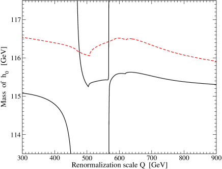
Figure 1: The real part $M_{h^{0}}$ of the pole mass of the lightest Higgs boson of supersymmetry for the sample test model of Ref. Martin:2002iu , as a function of the choice of renormalization scale $Q$. The solid line is the result of the calculation presented here. The dashed line shows the result if all effects involving electroweak couplings and lepton and slepton interactions are removed from the two-loop contribution, corresponding to previous approximations.

A striking feature of the graph is the presence of instabilities near $Q=463$ GeV (where the tree-level squared mass of $h^{0}$ passes through 0), and $Q=568$ GeV (where the Landau-gauge tree-level squared masses of the Nambu-Goldstone bosons $G^{0},G^{\pm}$ pass through 0) . The point is that for small tree-level scalar squared masses $m^{2}_{\phi}$, the effective potential scales like

$$V^{(2)}=\sum_{\phi}m^{2}_{\phi}[c^{\phi}_{1}\overline{\rm ln}(m_{\phi}^{2})+c^{\phi}_{2}\overline{\rm ln}^{2}(m_{\phi}^{2})]+\ldots$$ (20)

where $c^{\phi}_{1,2}$ are constants as $m^{2}_{\phi}\rightarrow 0$. Thus, while $V_{\rm eff}$ is well-defined and continuous in that limit, derivatives of it are not. (The Nambu-Goldstone bosons have $c^{\phi}_{2}=0$, so the corresponding singularities are less severe.) These and nearby values of $Q$ simply represent bad choices, where the approximation being made for the pole mass is invalidated by large logarithms. If it were available, the use of $\Pi^{(2)}(p^{2}=s_{h^{0}})$, rather than the approximation $\Pi^{(2)}(0)$, would eliminate the instability for choices of renormalization scale at which the Goldstone boson masses happen to vanish. [This is easily checked for the analogous case at one-loop order, where replacing $\Pi^{(1)}(p^{2})$ by $\Pi^{(1)}(0)$ leads to similar but milder numerical instabilities, because of $V^{(1)}=\sum_{\phi}(m^{2}_{\phi})^{2}\overline{\rm ln}(m_{\phi}^{2})/4+\ldots$ for $m_{\phi}^{2}\rightarrow 0$.] Therefore, one should simply be careful to avoid such choices for the renormalization scale .

For larger $Q$, the result for $M_{h^{0}}$ is nicely stable. A likely good range of scale choices is 600 GeV $<Q<$ 700 GeV. This range includes the geometric mean of the top-squark masses, a traditional guess for the optimal scale for evaluating $M_{h^{0}}$. It also includes the scale at which $M_{h^{0}}$ is equal to the tree-level value $m_{h^{0}}$, and the scale at which the two-loop corrections to the Goldstone boson masses vanish. In this range, the value of $M_{h^{0}}$ calculated by the method described here varies by less than 100 MeV. Even for the larger range 600 GeV $<Q<$ 900 GeV, the variation of $M_{h^{0}}$ is about 320 MeV. For reference, the precise result of the calculation at $Q_{0}=640$ GeV is $M_{h^{0}}=115.628$ GeV in this model.

For comparison, also shown in Figure 1 as the dashed line is the result which should correspond to previous approximations Zhang:1998bm ; Degrassi:2001yf in which electroweak, tau, stau, and tau sneutrino interactions $(g,g^{\prime},y_{\tau},a_{\tau})$ are neglected in the two-loop part . Because the terms implicated in eq. (20) are simply not included in this approximation, the instabilities of the full calculation at special values of $Q$ do not appear. The more important comparison occurs at the better choice of larger $Q$ as in the previous paragraph. There, the dashed-line estimate is significantly larger, and shows a stronger scale-dependence, than the calculation presented here with the complete $V^{(2)}$.

I have checked that similar results are obtained in a wide variety of MSSM models with dimensional parameters at or below the TeV scale, including models with larger and smaller $\tan\beta$ and different superpartner mass hierarchies and mixing angles. I find that the calculated $M_{h^{0}}$ is quite generally stable to within a few hundred MeV or less over a wide range which includes the geometric mean of the top squark masses and excludes any scales where tree-level scalar squared masses vanish. However, the scale-dependence of $M_{h^{0}}$ should not be confused with the actual theoretical error, which is probably somewhat larger. This is because some fraction of the neglected contributions is going to be scale-independent.

To improve the situation still further, one must calculate the full two-loop self-energies $\Pi^{(2)}(p^{2})$. The present work has shown that the effects of the electroweak couplings in this are certainly not negligible compared to our eventual ability to measure $M_{h^{0}}$ at colliders. The method outlined here will also be a useful check on a future calculation of $\Pi^{(2)}(p^{2})$ in Landau gauge, since it will have to coincide with the $p^{2}\rightarrow 0$ limit.

The viability of any given model scenario can be tested by conducting global fits of $M_{h^{0}}$ and many other observable masses, cross-sections, and decay rates to a set of underlying model parameters. If supersymmetry is part of our future, then the determination of $M_{h^{0}}$ will play an important role in testing the whole structure of the softly-broken supersymmetric Lagrangian.

References

• (1) H. E. Haber and G. L. Kane, Phys. Rept.  117, 75 (1985); J. F. Gunion and H. E. Haber, Nucl. Phys. B 272, 1 (1986) [Erratum-ibid. B 402, 567 (1993)]; S.P. Martin, “A supersymmetry primer,” [hep-ph/9709356].
• (2) R. Hempfling and A. H. Hoang, Phys. Lett. B 331, 99 (1994) [hep-ph/9401219]. H. E. Haber, R. Hempfling and A. H. Hoang, Z. Phys. C 75, 539 (1997) [hep-ph/9609331].
• (3) R.J. Zhang, Phys. Lett. B 447, 89 (1999) [hep-ph/9808299]; J.R. Espinosa and R.J. Zhang, JHEP 0003, 026 (2000) [hep-ph/9912236]; Nucl. Phys. B 586, 3 (2000) [hep-ph/0003246].
• (4) S. Heinemeyer, W. Hollik and G. Weiglein, Phys. Rev. D 58, 091701 (1998) [hep-ph/9803277]. Phys. Lett. B 440, 296 (1998) [hep-ph/9807423]. Eur. Phys. J. C 9, 343 (1999) [hep-ph/9812472].
• (5) A. Pilaftsis and C. E. Wagner, Nucl. Phys. B 553, 3 (1999) [hep-ph/9902371]. M. Carena, J. R. Ellis, A. Pilaftsis and C. E. Wagner, Nucl. Phys. B 586, 92 (2000) [hep-ph/0003180], Nucl. Phys. B 625, 345 (2002) [hep-ph/0111245].
• (6) M. Carena et al, Nucl. Phys. B 580, 29 (2000) [hep-ph/0001002].
• (7) J. R. Espinosa and I. Navarro, Nucl. Phys. B 615, 82 (2001) [hep-ph/0104047].
• (8) G. Degrassi, P. Slavich and F. Zwirner, Nucl. Phys. B 611, 403 (2001) [hep-ph/0105096], A. Brignole, G. Degrassi, P. Slavich and F. Zwirner, Nucl. Phys. B 631, 195 (2002) [hep-ph/0112177], Nucl. Phys. B 643, 79 (2002) [hep-ph/0206101].
• (9) S.P. Martin, Phys. Rev. D 65, 116003 (2002) [hep-ph/0111209].
• (10) S. P. Martin, Phys. Rev. D 66, 096001 (2002) [hep-ph/0206136].
• (11) W. Siegel, Phys. Lett. B 84, 193 (1979); D. M. Capper, D. R. Jones and P. van Nieuwenhuizen, Nucl. Phys. B 167, 479 (1980).
• (12) I. Jack et al, Phys. Rev. D 50, 5481 (1994) [hep-ph/9407291].
• (13) P. Chankowski, S. Pokorski and J. Rosiek, Nucl. Phys. B 423, 437 (1994) [hep-ph/9303309].
• (14) D.M. Pierce, J.A. Bagger, K.T. Matchev and R.J. Zhang, Nucl. Phys. B 491, 3 (1997) [hep-ph/9606211].
• (15) S.P. Martin and M.T. Vaughn, Phys. Rev. D 50, 2282 (1994) [hep-ph/9311340].