Improved Determination of the Mass of the $1^{-+}$ Light Hybrid Meson From QCD Sum Rules

Abstract

We calculate the next-to-leading order (NLO) $\alpha_{s}$-corrections to the contributions of the condensates $\langle\alpha G^{2}\rangle$ and $\langle\bar{q}q\rangle^{2}$ in the current-current correlator of the hybrid current $g\bar{q}(x)\gamma_{\nu}iF_{\mu\nu}^{a}T^{a}q(x)$ using the external field method in Feynman gauge. After incorporating these NLO contributions into the Laplace sum-rules, the mass of the $J^{PC}$=$1^{-+}$ light hybrid meson is recalculated using the QCD sum rule approach. We find that the sum rules exhibit enhanced stability when the NLO $\alpha_{s}$-corrections are included in the sum rule analysis, resulting in a $1^{-+}$ light hybrid meson mass of approximately 1.6 GeV.

I Introduction

Soon after Quantum Chromodynamics (QCD) became established as the theory of strong interactions, the search for mesons with exotic $J^{PC}$ quantum numbers was initiated. Important experimental progress has occurred in identifying potential candidates for exotic mesons. Among these are the two $J^{PC}=1^{-+}$ isovector states $\hat{\rho}(1405)$ and $\hat{\rho}(1600)$ which have been identified by two collaborations in the channels $\rho\pi$, $\eta\pi$ and $\eta^{\prime}\pi$ bnl1 ; bnl2 ; bnl3 . This gives the theorists an opportunity to compare their results for the exotic light hybrid mesons with the experimental observations. For instance, the widely cited mass prediction for the $J^{PC}=1^{-+}$ state from lattice QCD lies around 1.9 GeV lattice which disagrees with the experimental data. The decays of the $1^{-+}$ hybrid meson have also been studied in the context of various models page ; ailin , and also appear to be in disagreement with the experimental data. A possible reason for these inconsistencies may derive from the fact that non-perturbative effects cannot be easily controlled at this low energy scale. A further possibility is, of course, that the two new states may have been misidentified and are not hybrid mesons after all. It is clear that further theoretical studies of the properties of the hybrid mesons are necessary before one can be confident of their discovery.

In this paper, we concentrate on the mass prediction for the $1^{-+}$ hybrid meson using the QCD Laplace sum rule approach shif . Previous theoretical studies found masses in the range 1.4–2.1 GeV lead , with more recent estimates around 1.6 GeV narison ; jin . These latter estimates are close to the $\hat{\rho}(1600)$ but do not accommodate the state $\hat{\rho}(1405)$ as a hybrid candidate. However, the QCD sum rule analysis is not very stable, which from sum-rule studies of scalar gluonium and the $\rho$ meson, could be attributed to the importance of NLO corrections associated with the dimension-four $\langle\alpha_{s}G^{2}\rangle$ and dimension-six $\langle\bar{q}q\rangle^{2}$ operators chen ; glue . In particular, the four-quark operator has the same dimension as the two point correlator of the $1^{-+}$ current and its coefficient function is non-logarithmic in the leading order. Thus the dimension-six contributions are absent in the next-to-lowest moment sum-rule, resulting in discrepancies with the mass prediction from the zeroth moment sum rule lead . Thus it is interesting to determine whether the $\alpha_{s}$-corrections can reduce this discrepancy. For consistency, the $\alpha_{s}$-corrections to both the dimension-four $\langle\alpha_{s}G^{2}\rangle$ and the dimension-six $\langle\bar{q}q\rangle^{2}$ operators need to be included.

In this paper, we first give a brief introduction to the external field method used for our calculations. We then present our calculations for the $\alpha_{s}$ corrections to $\langle\bar{q}q\rangle^{2}$ and $\langle\alpha_{s}G^{2}\rangle$. Finally, we discuss the effect of the $\alpha_{s}$-corrections on the mass prediction for the $1^{-+}$ hybrid meson.

II External field method

In order to obtain the contribution of the operator $\alpha_{s}G^{a\mu\nu}G^{a}_{\mu\nu}$ in the Operator Product Expansion (OPE) expansion of the relevant current-current correlator, it is convenient to use the so-called external field method introduced in Ref. shif1 . Because we will use a slightly modified version of the external field method, we give a brief introduction to this method before carrying out our calculations. We first split the gauge field $A_{\mu}^{a}$ into two parts

$$A_{\mu}^{a}=(A_{\mu}^{a})_{ext}+a_{\mu}^{a},$$ (1)

where $(A_{\mu}^{a})_{ext}$ is an external (classical) field and $a_{\mu}^{a}$ is a quantum field. In the following we will suppress the label “ext” in $(A_{\mu}^{a})_{ext}$ for convenience. Substituting (1) in the QCD Lagrangian one obtains

$$L=-\frac{1}{4}F^{a\mu\nu}F^{a}_{\mu\nu}+\bar{\psi}i\hbox{$D\kern-7.0pt/$}\psi$$ (2)

where

$$F_{\mu\nu}={\frac{1}{ig}[D_{\mu},D_{\nu}]}\quad,\quad D_{\mu}=\partial_{\mu}+iga_{\mu}+igA_{\mu}$$ (3)

The Lagrangian (2) is invariant under the transformation

$$a_{\mu}(x)\rightarrow a^{\prime}_{\mu}=U^{-1}(x)(a_{\mu}(x)+A_{\mu}(x))U(x)-A_{\mu}(x)+\frac{i}{g}U^{-1}(x)U(x),$$ (4)

$$\psi(x)\rightarrow\psi^{\prime}=U(x)\psi(x),$$ (5)

$$A_{\mu}\rightarrow A^{\prime}_{\mu}(x)=A_{\mu}(x)\quad.$$ (6)

Unlike in shif1 , we demand that the external field is invariant under the gauge transformation. Therefore, any gauge condition imposed on the external field does not break the invariance under the gauge transformation (4). This is consistent with the result given in ste2 , which states that the series of the OPE for a correlator of gauge invariant currents does not depend on the choice the gauge of the external field. Furthermore, in order to fix the gauge of the quantum field, we use the Feynman gauge

$${-\frac{1}{2}(\partial_{\mu}a^{\mu})^{2}}$$ (7)

instead of the background gauge $-\frac{1}{2}(D^{ext}_{\mu}a^{\mu})^{2}$ used in shif1 , where $D^{ext}_{\mu}=\partial_{\mu}+igA_{\mu}$. This has the advantage that it can be shown that the external method in the covariant gauge is equivalent to the plane-wave method ste2 . Note that, when the external field method is used, the background gauge very likely differs from the covariant gauge in processes where both the radiation field and the external field are present in the initial states and (or) the final states. In the processes where only the radiation field or the external field is present in the initial states and (or) the final states, there is no difference between the background gauge and the covariant gauge. For instance, if there is only the external field present in the initial and (or) final states, the radiation field is integrated out. Then the external method in the background gauge is exactly the same as the original background gauge method back . The later is consistent with the plane-wave method. If there is only the radiation field present in the initial state and (or) final state, we can switch off the external field. Then there is no difference between the background gauge and the covariant gauge.

The Feynman rules in the Feynman gauge can be obtained quite straightforwardly. Under the infinitesimal gauge transformation

$$\delta a^{a}_{\mu}=-f^{abc}\omega^{b}(a^{c}_{\mu}+A^{c}_{\mu})+\frac{1}{g}\partial_{\mu}\omega^{a},$$ (8)

one can easily derive the Lagrangian for the ghost field

$$L_{ghost}=-\theta^{\dagger}_{a}[\partial^{2}\delta^{ab}-\hbox to0.0pt{\raise 7.0pt\hbox{$\leftarrow$}\hss}\partial f^{acb}(a^{c}_{\mu}+A^{c}_{\mu})]\theta_{b}.$$ (9)

Then, the external field $A_{\mu}$ obeys the same Feynman rules as the radiation field $a_{\mu}$. This is also consistent with the plane-wave method ste2 . The calculational techniques using the Lagrangian (2) are similar to those in the background gauge back .

In order to extract the operator $\alpha_{s}G^{a\mu\nu}G^{a}_{\mu\nu}$ from the OPE, the Fock-Schwinger condition is imposed on the external field

$$x^{\mu}A^{a}_{\mu}(x)=0.$$ (10)

Then, with the aid of the technique proposed in shif1 , the gluon propagator in the presence of the external field can be obtained straightforwardly. For instance, up to the term ${\cal O}(q^{-4})$ the gluon propagator is given by

$$\begin{split}D_{\mu\nu}(q,y)&=\int{\mathrm{e}}^{iq\cdot x}\mathrm{d}^{D}x\,\langle 0|Ta^{a}_{\mu}(x)a^{b}_{\nu}(y)|0\rangle\\ &=\frac{-i}{q^{2}}\left[\delta^{ab}g_{\mu\nu}-\frac{3}{2}\frac{G^{ab}_{\mu\nu}}{q^{2}}+\frac{q^{\rho}(G^{ab}_{\rho\mu}q_{\nu}+G^{ab}_{\rho\nu}q_{\mu})}{q^{4}}-\frac{iy^{\rho}}{2}\frac{(G^{ab}_{\rho\mu}q_{\nu}+G^{ab}_{\rho\nu}q_{\mu})}{q^{2}}+g_{\mu\nu}iy^{\rho}G^{ab}_{\rho\sigma}\frac{q^{\sigma}}{q^{2}}\right],\end{split}$$ (11)

where $G^{ab}_{\mu\nu}=gf^{acb}G^{c}_{\mu\nu}$ and $D=4-2\epsilon$ is the dimension of space-time. As expected, the gluon propagator (11) differs from the corresponding one given in shif1 . Sometimes it is more convenient to do the calculation in coordinate space. The gluon propagator in coordinate space can be obtained by using the $D$-dimensional Fourier transformation

$$D_{\mu\nu}(x,y)=\int\frac{\mathrm{d}^{D}q}{(2\pi)^{D}}{\mathrm{e}}^{-iq\cdot x}D_{\mu\nu}(q,y)$$ (12)

The necessary integration techniques in $D$-dimension were given in shif1 . One can convert the 4-dimensional quark propagator given in shif1 to the $D$-dimensional quark propagator

$$S(x,0)={\frac{\Gamma(\frac{D}{2})}{2\pi^{\frac{D}{2}}}\frac{\hbox{$x\kern-6.0pt/$}}{(x^{2})^{\frac{D}{2}}}-\frac{\Gamma(\frac{D}{2}-1)}{8\pi^{\frac{D}{2}}}\frac{x_{\alpha}{\tilde{G}}^{\alpha\beta}\gamma^{\beta}\gamma_{5}}{(x^{2})^{\frac{D}{2}-1}}}.$$ (13)

III NLO $O(\alpha_{s})$ corrections to $\langle G^{2}\rangle$ and $\langle\bar{q}q\rangle^{2}$

The two point correlator of the $1^{-+}$ hybrid current is defined as

$$\begin{split}\Pi_{\mu\nu}(q^{2})&=i\int\mathrm{d}^{4}x\,{\mathrm{e}}^{iqx}\langle 0|T\{j^{ren}_{\mu}(x),j^{ren+}_{\nu}(0)\}|0\rangle\\ &={(q_{\mu}q_{\nu}-g_{\mu\nu}q^{2})\Pi_{v}(Q^{2})+q_{\mu}q_{\nu}\Pi_{s}(q^{2})},\end{split}$$ (14)

where the current $j_{\mu}(x)=\bar{q}(x)T^{a}\gamma_{\nu}igF^{a}_{\mu\nu}q(x)$ carries isospin $I=1$ and the invariants $\Pi_{v}(Q^{2})$ and $\Pi_{s}(Q^{2})$ correspond to the contributions from $1^{-+}$ and $0^{++}$ states respectively. The renormalized current is denoted by $j^{ren}_{\mu}(x)$, which in the massless quark limit, has the form

$$j^{ren}_{\mu}=Zj_{\mu},$$ (15)

where up to the order ${\cal O}(\alpha_{s})$ and in the Feynman gauge the renormalization constant $Z$ is given by jin

$$Z={1+\frac{2}{9}\frac{g^{2}}{\pi^{2}}\frac{1}{\epsilon}}$$ (16)

The leading order calculation of (14) including the quark and gluon condensate contributions are contained in lead , and the NLO corrections to the perturbative part of (14) were calculated in narison ; jin . Next we consider the NLO corrections to the gluonic condensate $\langle\alpha_{s}G_{\mu\nu}G^{\mu\nu}\rangle$ contributions. We divide the calculations into two parts. One part can be obtained via the calculations of Feynman diagrams shown in Figure 1, where we do not display diagrams which vanish in dimensional regularization or which can be obtained from diagrams a–o in Fig. 1 by symmetry arguments. Because the expansion in term of $x_{\mu}$ violates translation invariance, the Fig. 1 diagrams g, j, and k respectively differ from diagrams m, n, and o. A straightforward calculation results in the structure

$$\begin{split}\Pi^{G^{2}}_{\mu\nu}(q^{2})=&\left(\frac{q_{\mu}q_{\nu}}{q^{2}}-g_{\mu\nu}\right)\alpha_{s}G_{\alpha\beta}G^{\alpha\beta}\Pi^{G^{2}}_{1}(q^{2})+\left(\frac{q_{\mu}q_{\nu}}{q^{2}}-g_{\mu\nu}\right)\alpha_{s}G_{\rho\beta}G_{\sigma}^{\beta}q^{\rho}q^{\sigma}\Pi^{G^{2}}_{2}(q^{2})\\ &+\left(\alpha_{s}G_{\mu\beta}G_{\nu}^{\beta}-\frac{q_{\mu}q_{\nu}}{q^{2}}\alpha_{s}G_{\rho\beta}G_{\sigma}^{\beta}q^{\rho}q^{\sigma}\right)\Pi^{G^{2}}_{3}(q^{2})+\alpha_{s}G_{\mu\rho}G_{\nu\sigma}q^{\rho}q^{\sigma}\Pi^{G^{2}}_{4}(q^{2})\\ &+\frac{q_{\mu}q_{\nu}}{q^{2}}\alpha_{s}G_{\alpha\beta}G^{\alpha\beta}\Pi^{G^{2}}_{5}(q^{2})+\frac{q_{\mu}q_{\nu}}{q^{2}}\alpha_{s}G_{\rho\beta}G_{\sigma}^{\beta}q^{\rho}q^{\sigma}\Pi^{G^{2}}_{6}(q^{2}).\end{split}$$ (17)

In order to extract $\langle\alpha_{s}G_{\mu\nu}G^{\mu\nu}\rangle$, we need a condition for the gluonic vacuum expectation value which reads

$$G_{\mu\nu}G_{\rho\sigma}={\frac{1}{D(D-1)}G_{\alpha\beta}G^{\alpha\beta}(g_{\mu\rho}g_{\nu\sigma}-g_{\mu\sigma}g_{\nu\rho})}.$$ (18)

Then, in the $\rm\overline{MS}$-scheme and Feynman gauge, we obtain

$$\Pi^{G^{2}a}_{v}(q^{2})={-\frac{1}{36\pi}\ln\left(\frac{-q^{2}}{\mu^{2}}\right)\langle\alpha_{s}G^{2}\rangle\left[\frac{16}{9}\frac{\alpha_{s}(\mu)}{\pi}\ln\left(\frac{-q^{2}}{\mu^{2}}\right)-\frac{1139}{216}\frac{\alpha_{s}(\mu)}{\pi}\right]+{\rm infinite~{}terms}}$$ (19)

$$\Pi^{G^{2}a}_{s}(q^{2})={\frac{1}{24\pi}\ln\left(\frac{-q^{2}}{\mu^{2}}\right)\langle\alpha_{s}G^{2}\rangle\left[\frac{16}{9}\frac{\alpha_{s}(\mu)}{\pi}\ln\left(\frac{-q^{2}}{\mu^{2}}\right)-\frac{1459}{216}\frac{\alpha_{s}(\mu)}{\pi}\right]+{\rm infinite~{}terms}}\quad,$$ (20)

where $\langle\alpha G^{2}\rangle\equiv\langle\alpha G^{a}_{\mu\nu}G^{a\,\mu\nu}\rangle$. Another part of the next-to-leading order calculation of $\langle\alpha_{s}G_{\mu\nu}G^{\mu\nu}\rangle$ results from the renormalization of the current (15), i.e.

$$i\int\mathrm{d}^{4}x\,{\mathrm{e}}^{iqx}2(Z-1)\langle 0|T\{j_{\mu}(x),j^{+}_{\nu}(0)\}|0\rangle,$$ (21)

It reads

$$\Pi^{G^{2}b}_{v}(q^{2})={-\frac{1}{36\pi}\ln\left(\frac{-q^{2}}{\mu^{2}}\right)\langle\alpha_{s}G^{2}\rangle\left[-\frac{8\alpha_{s}(\mu)}{9\pi}\ln\left(\frac{-q^{2}}{\mu^{2}}\right)+\frac{88}{27}\frac{\alpha_{s}(\mu)}{\pi}\right]+{\rm infinite~{}terms}}$$ (22)

$$\Pi^{G^{2}b}_{s}(q^{2})={\frac{1}{24\pi}\ln\left(\frac{-q^{2}}{\mu^{2}}\right)\langle\alpha_{s}G^{2}\rangle\left[-\frac{8\alpha_{s}(\mu)}{9\pi}\ln\left(\frac{-q^{2}}{\mu^{2}}\right)+\frac{104}{27}\frac{\alpha_{s}(\mu)}{\pi}\right]+{\rm infinite~{}terms}},$$ (23)

where the sum of the infinite terms in (19) and (22) is scale-independent. We did not check on the infrared convergence of the sum of infinite terms because we used dimensional regularization. However, the sum of these two parts must be IR convergent so that the Wilson coefficient of the condensates only depends on short-distance effects. Obviously, this result is invariant if we use the background gauge, because all radiation fields are integrated out. We have checked such invariance.

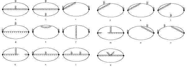
Figure 1: Feynman diagrams for the $\alpha_{s}$-corrections to the condensate $\langle\alpha_{s}G^{2}\rangle$. Dots stand for the current vertices.

Similarly, by calculating the Feynman diagrams shown in Fig. 2, we obtain the next-to-leading order corrections for the $\langle\bar{q}q\rangle^{2}$ contributions

$$\Pi^{q}_{v}(q^{2})={\frac{4\pi}{9q^{2}}\alpha_{s}(\mu)\langle\bar{q}q\rangle^{2}\left[\left(\frac{11}{72}+\frac{1}{6}n_{f}\right)\frac{\alpha_{s}(\mu)}{\pi}\ln\left(\frac{-q^{2}}{\mu^{2}}\right)+\left(\frac{91}{108}-\frac{5}{18}n_{f}\right)\frac{\alpha_{s}(\mu)}{\pi}\right]}$$ (24)

$$\Pi^{q}_{s}(q^{2})={-\frac{4\pi}{3q^{2}}\alpha_{s}(\mu)\langle\bar{q}q\rangle^{2}\left[\left(\frac{53}{72}+\frac{1}{6}n_{f}\right)\frac{\alpha_{s}(\mu)}{\pi}\ln\left(\frac{-q^{2}}{\mu^{2}}\right)-\left(\frac{14}{9}+\frac{1}{6}n_{f}\right)\frac{\alpha_{s}(\mu)}{\pi}\right]}\quad,$$ (25)

where we have used the vacuum saturation approximation

$$\langle\bar{q}_{i}^{a}q_{j}^{b}\bar{q}_{i^{\prime}}^{a^{\prime}}q_{j^{\prime}}^{b^{\prime}}\rangle={(\frac{1}{12})^{2}\langle\bar{q}q\rangle^{2}(\delta_{ij}\delta_{i^{\prime}j^{\prime}}\delta_{ab}\delta_{a^{\prime}b^{\prime}}-\delta_{ij^{\prime}}\delta_{i^{\prime}j}\delta_{ab^{\prime}}\delta_{a^{\prime}b})}\quad.$$ (26)

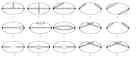
Figure 2: Feynman diagrams for the $\alpha_{s}$-corrections to the condensate$\langle\bar{q}q\rangle^{2}$. Dots stand for the current vertices.

IV Mass of the $1^{-+}$ hybrid mesons

QCD sum rules are based on the resonance plus continuum duality ansatz

$$\frac{1}{\pi}Im\Pi_{v,s}(s)=\sum_{R}M_{R}^{6}f_{R}^{2}\delta\left(s-M_{R}^{2}\right)+{\rm QCD~{}continuum},$$ (27)

where $M_{R}$ is the mass of the resonance $R$, $f_{R}$ denotes the coupling of the resonance to the current and we use the narrow resonance approximation $\delta(s-M_{R}^{2})$ for the resonance $R$. The spectral density $\rho_{v,s}(s)=\frac{1}{\pi}Im\Pi_{v,s}(s)$ can be related to the correlator $\Pi_{v,s}(q^{2})$ at the scale $-q^{2}$ via the standard dispersion relation

$$\Pi_{v,s}(q^{2})={(q^{2})^{n}\int^{\infty}_{0}ds\frac{\rho_{v,s}(s)}{s^{n}(s-q^{2})}+\sum^{n-1}_{k=0}a_{k}(q^{2})^{k}},$$ (28)

where the $a_{k}$ are appropriate subtraction constants to render Eq. (28) finite. The energy variable $-q^{2}$ has to be chosen in a region where one can incorporate the asymptotic freedom property of QCD via the operator product expansion. The spectral function $\Pi_{v,s}(q^{2})$ can be expressed as

$$\Pi_{v,s}(q^{2})=\sum_{dim~{}n}C_{n}(-q^{2},\mu){\it O}_{n}(\mu)$$ (29)

where the scale $\mu$ separates the long-distance and short distance regime of QCD. The Wilson coefficients $C_{n}(-q^{2},\mu)$ for the low dimension operators were given in lead ; jin as summarized in Section 3 of this paper. Ref.  narison also introduced a dimension two operator resulting from the resummation of the large order terms of the OPE series. However, this method appears to be model-dependent and could result in a double counting of the contribution of the operators considered in the present approach. We will therefore not include the dimension two term in our analysis.

Concentrating on the analysis of the vector $1^{-+}$ channel, the lowest-lying resonance in the spectral density is enhanced by the standard approach of applying the Borel transform operator to (28) weighted by powers of $q^{2}$ shif . This results in the Laplace sum-rules

$$R_{k}\left(\tau,s_{0}\right)=\int^{s_{0}}s^{k}{\mathrm{e}}^{-s\tau}\rho_{v}(s)\mathrm{d}s~{};~{}k=0,1,2,\ldots$$ (30)

where the quantity $R_{k}$ represents the QCD prediction, and the threshold $s_{0}$ separates the contribution from higher excited states and the QCD continuum. In the single narrow resonance scenario, the lowest-lying resonance mass can be obtained from ratios

$$M_{R}^{2}=\frac{R_{k+1}\left(\tau,s_{0}\right)}{R_{k}\left(\tau,s_{0}\right)}\quad.$$ (31)

The zero-weighted sum-rule $R_{0}$ for $n_{f}=3$ can be obtained from Eqs. (19) and (22), and Refs.lead ; jin , with some results needed for calculation of the necessary Borel transforms extracted from glue .

$$\begin{split}R_{0}\left(\tau,s_{0}\right)=&\frac{1}{240\pi^{2}}\frac{\alpha}{\pi}\left(1+\frac{1301}{240}\frac{\alpha}{\pi}\right)\int\limits_{0}^{s_{0}}t^{2}\mathrm{e}^{-t\tau}\mathrm{d}t-\frac{1}{120\pi^{2}}\frac{\alpha}{\pi}\left(\frac{17}{72}\frac{\alpha}{\pi}\right)\int\limits_{0}^{s_{0}}t^{2}\mathrm{e}^{-t\tau}\ln\left(\frac{t}{\mu^{2}}\right)\mathrm{d}t\\ &+\frac{1}{36\pi}\left(1-\frac{145}{72}\frac{\alpha}{\pi}\right)\langle\alpha G^{2}\rangle\int\limits_{0}^{s_{0}}\mathrm{e}^{-t\tau}\mathrm{d}t+\frac{1}{36\pi}\left(\frac{16}{9}\frac{\alpha}{\pi}\right)\langle\alpha G^{2}\rangle\int\limits_{0}^{s_{0}}\mathrm{e}^{-t\tau}\ln\left(\frac{t}{\mu^{2}}\right)\mathrm{d}t\\ &-\langle{\cal O}_{6}\rangle-\frac{4\pi}{9}\left(1+\frac{1}{108}\frac{\alpha}{\pi}\right)\alpha\langle\bar{q}q\rangle^{2}-\frac{4\pi}{9}\left(\frac{47}{72}\frac{\alpha}{\pi}\right)\alpha\langle\bar{q}q\rangle^{2}\left[-\gamma_{E}-\ln\left(\mu^{2}\tau\right)-E_{1}\left(s_{0}\tau\right)\right]\end{split}$$ (32)

The quantity $\langle{\cal O}_{6}\rangle$ is defined by

$$\langle{\cal O}_{6}\rangle=\frac{1}{192\pi^{2}}\langle g^{3}G^{3}\rangle-\frac{83}{1728}\frac{\alpha}{\pi}m_{q}\langle\bar{q}gGq\rangle\quad.$$ (33)

Renormalization-group improvement of (32) is achieved by setting $\mu^{2}=1/\tau$ RG , and higher-weight sum-rules can be obtained from $\tau$ derivatives of (32) before implementing renormalization-group improvement. As stated earlier, this procedure implies that the NLO $\alpha\langle\bar{q}q\rangle^{2}$ correction provides the leading contribution in $R_{1}$.

The various QCD parameters that will be used in the phenomenological analysis of (32) are

$$\Lambda_{{\overline{MS}}}\approx 0.3\,{\rm GeV}~{},~{}\alpha_{s}\langle\bar{q}q\rangle^{2}=1.8\times 10^{-4}\,{\rm GeV^{6}}~{},~{}m_{q}\langle\bar{q}q\rangle=-\frac{1}{4}f_{\pi}^{2}m_{\pi}^{2}$$ (34)

$$\langle\alpha_{s}G^{2}\rangle=0.07\,{\rm GeV^{4}}~{},~{}g^{3}\langle G^{3}\rangle=1.1\,{\rm GeV^{2}}\langle\alpha_{s}G^{2}\rangle~{},~{}f_{\pi}=0.132\,{\rm GeV}~{},~{}m_{q}\langle\bar{q}gGq\rangle=1.5\,{\rm GeV^{2}}m_{q}\langle\bar{q}q\rangle.$$ (35)

The parameter $\langle\alpha_{s}G^{2}\rangle$ represents the central value in the recent determination nar1 , $g^{3}\langle G^{3}\rangle$ is obtained from the dilute instanton gas model dilute , $\langle\bar{q}gGq\rangle$ is extracted from reind , and the dimension-six condensate parameter $\alpha_{s}\langle\bar{q}q\rangle^{2}$ is referenced to the vacuum saturation value which is known to underestimate the actual value by up to a factor of 2 in the ($I=1$) vector and axial vector channels saturation .

Before considering a detailed analysis of the sum-rules, we consider the $s_{0}\to\infty$ limit of the sum-rules which provides the following bound on the lightest resonance mass

$$M_{R}^{2}\leq\frac{R_{1}\left(\tau,\infty\right)}{R_{0}\left(\tau,\infty\right)}\quad,$$ (36)

which has the advantage of being a robust bound independent of the QCD continuum model. The explicit expressions for the sum-rules in the $s_{0}\to\infty$ limit are

$$\begin{split}R_{0}\left(\tau,\infty\right)=&\frac{1}{240\pi^{2}}\frac{\alpha}{\pi}\left(1+\frac{1301}{240}\frac{\alpha}{\pi}\right)\frac{2}{\tau^{3}}-\frac{1}{120\pi^{2}}\left(\frac{\alpha}{\pi}\right)^{2}\frac{17}{72}\left(3-2\gamma_{E}\right)\frac{1}{\tau^{3}}+\frac{1}{36\pi}\left(1-\frac{145}{72}\frac{\alpha}{\pi}\right)\langle\alpha G^{2}\rangle\frac{1}{\tau}\\ &-\frac{1}{36\pi}\frac{16}{9}\frac{\alpha}{\pi}\langle\alpha G^{2}\rangle\frac{\gamma_{E}}{\tau}-\langle{\cal O}_{6}\rangle-\frac{4\pi}{9}\left(1+\frac{1}{108}\frac{\alpha}{\pi}\right)\alpha\langle\bar{q}q\rangle^{2}+\frac{4\pi}{9}\left(\frac{47}{72}\frac{\alpha}{\pi}\right)\alpha\langle\bar{q}q\rangle^{2}\gamma_{E}\end{split}$$ (37)

$$\begin{split}R_{1}\left(\tau,\infty\right)=&\frac{1}{240\pi^{2}}\frac{\alpha}{\pi}\left(1+\frac{1301}{240}\frac{\alpha}{\pi}\right)\frac{6}{\tau^{4}}-\frac{1}{120\pi^{2}}\left(\frac{\alpha}{\pi}\right)^{2}\frac{17}{72}\left(11-6\gamma_{E}\right)\frac{1}{\tau^{4}}\\ &+\frac{1}{36\pi}\left(1-\frac{145}{72}\frac{\alpha}{\pi}\right)\langle\alpha G^{2}\rangle\frac{1}{\tau^{2}}-\frac{1}{36\pi}\frac{16}{9}\frac{\alpha}{\pi}\langle\alpha G^{2}\rangle\frac{1-\gamma_{E}}{\tau^{2}}-\frac{4\pi}{9}\left(\frac{47}{72}\frac{\alpha}{\pi}\right)\alpha\langle\bar{q}q\rangle^{2}\frac{1}{\tau}\quad.\end{split}$$ (38)

The effect of the NLO $\langle\alpha G^{2}\rangle$ and $\alpha\langle\bar{q}q\rangle^{2}$ corrections is illustrated in Figure 3, where it is observed that the mass bound is increased significantly when these higher-order corrections are included. For brevity, we respectively refer to sum-rules containing the NLO and LO $\langle\alpha G^{2}\rangle$ and $\alpha\langle\bar{q}q\rangle^{2}$ corrections as the NLO and LO sum-rules. In particular, we see from Fig. 3 that the $\hat{\rho}(1600)$, excluded for the LO case, can be accommodated when the NLO corrections are included. Furthermore, the minimum of the NLO bounds occurs at a reasonable energy ($\tau$) scale in contrast to the rather large energy scale occurring when only LO corrections are included.

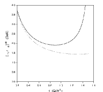
Figure 3: The ratio $\sqrt{R_{1}\left(\tau,\infty\right)/R_{0}\left(\tau,\infty\right)}$ as a function of $\tau$ for the NLO (solid curve) and LO (dashed curve) sum-rules. As discussed in the text, acceptable values of $M_{R}$ must lie below these curves.

The mass estimate $M_{R}$ is obtained by optimizing the choice of $s_{0}$ such that the most stable $R_{1}/R_{0}$ ratio is obtained. Figures 4 and 5 illustrate this ratio for selected values of $s_{0}$, resulting in $M_{R}\approx 1.6\,{\rm GeV}$ and $s_{0}\approx 4.0\,{\rm GeV^{2}}$ for the NLO case, while the LO analysis results in $M_{R}\approx 1.3\,{\rm GeV}$ and $s_{0}\approx 3.0\,{\rm GeV^{2}}$. These optimized values of $M_{R}$ are consistent with the bounds established in Fig. 3, and explicitly demonstrate that the NLO condensate effects raise the estimated value of the hybrid mass.

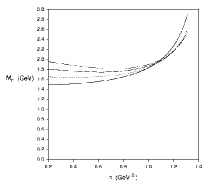
Figure 4: The NLO sum-rule ratio $\sqrt{R_{1}\left(\tau,s_{0}\right)/R_{0}\left(\tau,s_{0}\right)}$ as a function of $\tau$ for the sequence of $s_{0}$ values $s_{0}=\left\{3.0,~{}4.0,~{}5.0,~{}6.0\right\}\,{\rm GeV^{2}}$. The lowest (solid) curve corresponds to $s_{0}=3.0\,{\rm GeV^{2}}$, and the upper (dashed-dotted) curve corresponds to $s_{0}=6.0\,{\rm GeV^{2}}$.

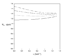
Figure 5: The LO sum-rule ratio $\sqrt{R_{1}\left(\tau,s_{0}\right)/R_{0}\left(\tau,s_{0}\right)}$ as a function of $\tau$ for the sequence of $s_{0}$ values $s_{0}=\{2.0~{},3.0,~{}4.0,~{}5.0\}\,{\rm GeV^{2}}$. The lowest (solid) curve corresponds to $s_{0}=2.0\,{\rm GeV^{2}}$, and the upper (dashed-dotted) curve corresponds to $s_{0}=6.0\,{\rm GeV^{2}}$.

The stability and self-consistency of the sum-rule analyses can be examined by using the optimized $s_{0}$ and $M_{R}$ as input into the following expressions resulting from the single resonance model.

$$\frac{\mathrm{e}^{-M_{R}^{2}\tau}}{M_{R}^{2k}}R_{k}\left(\tau,s_{0}\right)=f_{R}^{2}M_{R}^{6}$$ (39)

Figure 6 displays the left-hand side of (39) for the NLO $k=0,1,2$ sum-rules. We see from Fig. 6 that a stable ratio containing a $\tau$ critical point occurs for each value of $k$, and that the variation of the corresponding value of $f_{R}^{2}M_{R}^{6}$ with $k$ is minimal. By contrast, the corresponding curves for the LO sum-rules shown in Figure 7 do not exhibit a critical point in the same $\tau$ range associated with the Fig. 5 mass estimate, and show strong dependence on $k$. Thus the NLO $\langle\alpha G^{2}\rangle$ and $\alpha\langle\bar{q}q\rangle^{2}$ corrections lead to improved stability and self-consistency in the sum-rule analysis.

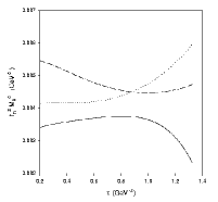
Figure 6: The quantity $M_{R}^{-2k}\mathrm{e}^{-M_{R}^{2}\tau}R_{k}\left(\tau,s_{0}\right)$, which in the single-resonance model corresponds to $f_{R}^{2}M_{R}^{6}$, is displayed as a function of $\tau$ for the $k=0,1,2$ NLO sum-rules. The optimized values $s_{0}=4.0\,{\rm GeV^{2}}$ and $M_{R}=1.64\,{\rm GeV}$ are used as inputs, the lowest (solid) curve corresponds to $k=0$, the intermediate (dotted) curve corresponds to $k=1$, and the upper (dashed) curve corresponds to $k=2$.

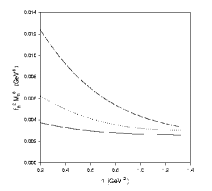
Figure 7: The quantity $M_{R}^{-2k}\mathrm{e}^{-M_{R}^{2}\tau}R_{k}\left(\tau,s_{0}\right)$, which in the single-resonance model corresponds to $f_{R}^{2}M_{R}^{6}$, is displayed as a function of $\tau$ for the $k=0,1,2$ LO sum-rules. The optimized values $s_{0}=3.0\,{\rm GeV^{2}}$ and $M_{R}=1.31\,{\rm GeV}$ are used as inputs, the lowest (solid) curve corresponds to $k=0$, the intermediate (dotted) curve corresponds to $k=1$, and the upper (dashed) curve corresponds to $k=2$.

The dominant uncertainties in the sum-rule analysis associated with the QCD parameters (34) and (35) are related to $\Lambda_{\overline{{\rm MS}}}$ and $\alpha\langle\bar{q}q\rangle^{2}$. If the pattern established in other sum-rule channels saturation is upheld for the hybrid OPE, then $\alpha\langle\bar{q}q\rangle^{2}$ given in (34) underestimates the true value. Similarly, $\Lambda_{\overline{{\rm MS}}}=300\,{\rm MeV}$ is a lower bound following from $\alpha_{s}\left(M_{\tau}\right)$ pdg . Increasing either of these parameters increases the hybrid mass estimates, and thus it appears difficult to accommodate the $\hat{\rho}(1400)$.

Finally, we have verified that the results of our analysis are essentially independent of the choice of renormalization scale $\mu^{2}=1/\tau$ motivated by renormalization-group improvement in the $s_{0}\to\infty$ limit RG . Choosing renormalization scales in the energy region near the hybrid mass has a minimal effect on the sum-rule analysis.

V Summary

The (NLO) $\alpha_{s}$ corrections to the $\langle\alpha_{s}G^{2}\rangle$ and $\alpha\langle\bar{q}q\rangle^{2}$ contributions in the two point correlator of the current $g\bar{q}\gamma_{\nu}iG_{\mu\nu}^{a}T^{a}q(x)$ have been calculated, and the effect of these contributions on the QCD sum-rule estimates of the $1^{-+}$ hybrid mass have been examined. The NLO $\alpha\langle\bar{q}q\rangle^{2}$ corrections are particularly interesting since they provide the leading contributions to the $R_{1}$ sum-rule. The NLO $\langle\alpha_{s}G^{2}\rangle$ and $\alpha\langle\bar{q}q\rangle^{2}$ contributions improve the stability and self-consistency of the sum-rule analysis, resulting in a $1^{-+}$ hybrid mass of approximately $1.6\,{\rm GeV}$. This result reflects a lower bound devolving from the QCD input parameters, so it appears difficult to accommodate the $\hat{\rho}(1400)$ as a hybrid state.

References

(1)
D. R. Thompson et al. (E852 Collab.), Phys. Rev. Lett. 79 (1997)
1630.
A. Abele et al. (Crystal Barrel Collab.), Phys. Lett. B423 (1998)
175.
(2)
G.S. Adams et al (E852 Collab.), Phys. Rev. Lett. 81 (1998)
5760.
(3) E.I. Ivanov. et al, (E852 Collab.), Phys. Rev. Lett.
86 (2001) 3977.
(4)
P. Lacock et al (UKQCD Collaboration), Phys. Lett. B401 (1997) 308;
C. Bernard et al,
(MILC Collaboration), Phys. Rev. D56 (1997) 7039;
K.J. Juge, J. Kuti, C.J. Morningstar, Proceedings of HADRON97 (hep-ph/9711451);
P. Lacock et al, (SESAM
Collab.), Nucl. Phys. Proc. Suppl. 73 (1999) 261;
C. Michael et al Nucl. Phys. A655 (1999) 12;
C. Bernard et al, Phys. Rev. D56 (1997) 7039;
C. McNeilie et al Phys. Rev. D65 (2002) 094505;
Z.H. Mei and Z.Q. Luo, hep-lat/0206012.
(5)
F. E. Close and P. R. Page, Nucl. Phys. B443 (1995) 233;
P. R. Page, E. S. Swanson, A. P. Szczepaniak, Phys. Rev. D59 (1999) 034016
(6) Ailin Zhang and T. G. Steele, Phys. Rev. D65 (2002) 114013;
Ailin Zhang and T. G. Steele, hep-ph/0207369.
(7)
M. A. Shifman, A. I. Vainshtein and V. I. Zakharov, Nucl. Phys. B147
(1979) 385.
(8)
J. Govaerts, F. de Viron, D. Gushin and J. Weyers, Phys. Lett. B128 (1984) 262;
J. Govaerts, F. de Viron, D. Gushin and J. Weyers, Nucl. Phys. B248 (1984) 1;
I.I. Balitsky, D.I. Dyakonov, A.V. Yung, Z. Phys. C33 (1986) 265;
J.I. Latorre, S. Narison and P. Pascual, Z. Phys. C34 (1987) 347;
J. Govaerts, L.J. Reinders, P. Franken, X. Gonze and J. Weyers, Nucl.
Phys. B284 (1987) 674.
(9)
S. Narison, Nucl. Phys. A675 (2000) 54c;
K. Chetyrkin and S. Narison, Phys. Lett. B485 (2000) 145.
(10) H. Y. Jin and J. G. Körner, Phys. Rev. D64 (2001) 074002.
(11) L. V. Lanin, V. P. Spiridonov and K. G. Chetyrkin, Yad Fiz.
44 (1986) 1372.
(12)
E. Bagan and T. G. Steele, Phys. Lett. B243 (1990) 413.
(13) V. A. Novikov, M. A. Shifman et al.,
Fortschr. Phys. 32 (1984) 11.
(14) E. Bagan , M.R. Ahmady,
V. Elias, T.G. Steele, Z.Phys. C61 (1994) 157.
(15) L. F. Abbott, Nucl. Phys. B185 (1981) 189;
R. Tarrach, Nucl. Phys. B196 (1982) 45.
(16) S. Narison and E. de Rafael, Phys. Lett. B103 (1981) 57.
(17) S. Narison, Nucl. Phys. Proc. Supp. A54 (1997) 238.