The Resummed Photon Spectrum in Radiative $\Upsilon$ Decays

Abstract

We present a theoretical prediction for the photon spectrum in radiative $\Upsilon$ decay including the effects of resumming the endpoint region, $E_{\gamma}\to M_{\Upsilon}/2$. Our approach is based on NRQCD and the soft collinear effective theory. We find that our results give much better agreement with data than the leading order NRQCD prediction.

The radiative decay $\Upsilon\to X\gamma$ was first investigated about a quarter century ago firstRad . The conventional wisdom at was that this process is computable in perturbative QCD due to the large mass of the $b$ quarks. Since then, we have learned much about quarkonium in gerneral bbl and this process in particular Catani:1995iz ; Maltoni:1999nh ; Rothstein:1997ac ; Kramer:1999bf ; Bauer:2001rh . In addition, CLEO is currently taking data on the low lying $\Upsilon$ resonances and will soon be able to update their original measurement of this decay Nemati:1996xy . It is thus timely to reexamine the theoretical predictions for this rate.

The current method for calculating the direct radiative decay of the $\Upsilon$ is by using the operator product expansion (OPE), with the operators scaling as some power of the relative velocity of the heavy quarks, $v$, given by the power counting of Non-Relativistic QCD (NRQCD) bbl . The $v\to 0$ limit of NRQCD coincides with the color-singlet (CS) model calculation of firstRad .

This picture is only valid in the intermediate range of the photon energy ($0.3\lesssim z\lesssim 0.7$, where $z=2E_{\gamma}/M$, and $M=2m_{b}$). In the lower range, $z\lesssim 0.3$, photon-fragmentation contributions are important Catani:1995iz ; Maltoni:1999nh . At large values of the photon energy, $z\gtrsim 0.7$, both the perturbative expansion Maltoni:1999nh and the OPE Rothstein:1997ac break down.

The breakdown at large $z$ is due to NRQCD not including collinear degrees of freedom. The correct effective field theory is a combination of NRQCD for the heavy degrees of freedom and the soft-collinear effective theory (SCET) Bauer:2001ew ; Bauer:2001ct for the light degrees of freedom. In a previous paper Bauer:2001rh we applied SCET to the color-octet (CO) contributions to radiative $\Upsilon$ decay. Here we treat the CS contribution at the endpoint within SCET. In this letter we present the main results of the analysis, and leave the details to a companion paper FL .

The inclusive photon spectrum can be written as a sum of a direct and a fragmentation contribution Catani:1995iz ,

$$\frac{d\Gamma}{dz}=\frac{d\Gamma^{\rm dir}}{dz}+\frac{d\Gamma^{\rm frag}}{dz},$$ (1)

where in the direct term the photon is produced in the hard scattering, and in the fragmentation term the photon fragments from a parton produced in the initial hard scattering. The fragmentation contribution has been well studied in Ref. Maltoni:1999nh , and we do not add anything new here.

The direct contribution can be calculated using the OPE, where the rate can be written as

$$\frac{d\Gamma}{dz}=\sum_{n}C_{n}(M,z)\langle\Upsilon|{\cal O}_{n}|\Upsilon\rangle\,.$$ (2)

The $C_{i}$ are short-distance coefficients, calculable as a perturbative series in $\alpha_{s}(M)$, and the ${\cal O}$ are NRQCD operators, scaling with specific powers of $v\ll 1$.

At leading order in $v$ only a CS term contributes. The CS operator ${\cal O}(1,{}^{3}S_{1})$ creates and annihilates a CS quark-antiquark pair in a ${}^{3}S_{1}$ configuration, and is multiplied by the CS coefficient, which at leading order is proportional to $\alpha^{2}_{s}(M)$. There are also CO contributions down by $v^{4}$. Two of these, proportional to the CO ${}^{1}S_{0}$ and ${}^{3}P_{0}$ matrix elements (MEs), give rise to large enhancement at the endpoint Maltoni:1999nh . Since the CO ${}^{1}S_{0}$ and ${}^{3}P_{0}$ MEs are unknown, and since the data does not show any enhancement near the upper endpoint, we set them to zero. However, we include the CO ${}^{3}S_{1}$ ME. It has a sizable fragmentation contribution, but becomes negligible as $z$ increases, and thus does not conflict with data Maltoni:1999nh .

The lowest order CS direct rate is firstRad

$$\frac{1}{\Gamma_{0}}\frac{d\Gamma^{\rm dir}_{\rm LO}}{dz} = \frac{2-z}{z}+\frac{z(1-z)}{(2-z)^{2}}+2\frac{1-z}{z^{2}}\ln(1-z)$$ (3)

$$-2\frac{(1-z)^{2}}{(2-z)^{3}}\ln(1-z),$$

where

$$\Gamma_{0}=\frac{32}{27}\alpha\alpha_{s}^{2}e_{b}^{2}\frac{\langle\Upsilon|{\cal O}_{1}(^{3}S_{1})|\Upsilon\rangle}{m_{b}^{2}},$$ (4)

and $e_{b}=-1/3$. The ME is related to the wavefunction

$$\langle\Upsilon|{\cal O}_{1}(^{3}S_{1})|\Upsilon\rangle=\frac{N_{c}}{2\pi}|R(0)|^{2}.$$ (5)

The $\alpha_{s}$ correction to this rate was calculated numerically in Ref. Kramer:1999bf , leading to small corrections over most of phase space. In the endpoint region, however, the corrections are of order the leading contribution.

In the endpoint region, the outgoing gluons are moving back-to-back to the photon, with large energy and small invariant mass (ie, a collinear jet). We must, therefore, couple NRQCD to SCET Bauer:2001ct . The scales, set by the lightcone momentum components of the collinear particles, are widely separated. If we choose $p^{-}$ to be ${\cal O}(M)$, then $p_{\perp}/p^{-}\sim\lambda$, and $p^{+}/p^{-}\sim\lambda^{2}$, where $\lambda$ is a small parameter. Here the collinear scale is

$$\mu_{c}\sim M\sqrt{1-z}\sim\sqrt{M\Lambda_{\rm QCD}}\,.$$ (6)

Thus $\lambda$ is of order $\sqrt{1-z}\sim\sqrt{\Lambda_{\rm QCD}/M}$.

There are two types of fundamental objects in SCET (fields and Wilson lines) and two separate sectors (collinear and usoft). In the collinear sector there is a fermion field $\xi_{n,p}$, a gluon field $A_{n,q}^{\mu}$, and a Wilson line

$$W_{n}(x)=\bigg{[}\sum_{\rm perms}{\rm exp}\left(-g_{s}\frac{1}{\bar{\cal P}}{\bar{n}}\cdot A_{n,q}(x)\right)\bigg{]}\,.$$ (7)

Collinear fields are labeled by a direction $n^{\mu}$ and the large components (${\bar{n}}\cdot q,q_{\perp}$). The operator ${\cal P}^{\mu}$ projects out the momentum label. Likewise in the usoft sector there is a fermion field $q_{us}$, a gluon field $A^{\mu}_{us}$, and a Wilson line $Y$. Operators are constructed out of these objects such that they are gauge invariant. Thus, operators with collinear gluons are built out of the homogeneous (order $\lambda$) component of the collinear field strength, $\bar{\cal P}B^{\mu}_{\perp}\equiv{\bar{n}}_{\nu}G^{\nu\mu}_{n}$ Bauer:2002nz ,

$$B^{\mu}_{\perp}=\frac{-i}{g_{s}}W^{\dagger}({\cal P}_{\perp}^{\mu}+g_{s}(A^{\mu}_{n,q})_{\perp})W.$$ (8)

We now write down the leading operator. Aside from $B_{\perp}$, we also need the NRQCD heavy quark and antiquark fields, $\psi_{\bf p}$ and $\chi_{-{\bf p}}$, which transform only under usoft (not collinear) gauge transformations. A CS ${}^{3}S_{1}$ $b\bar{b}$ pair decays into a photon and a colorless jet of gluons. We must, therefore, include two of the $B_{\perp}$ fields in a colorless configuration, and the only operator is

$${\cal O}(1,{}^{3}S_{1}) =$$

$$\chi^{\dagger}_{-{\bf p}}\mbox{\boldmath$\sigma$}^{\delta}\psi_{\bf p}{\rm Tr}\big{\{}B^{\alpha}_{\perp}\,\Gamma^{(1,{}^{3}S_{1})}_{\alpha\beta\delta\mu}(\bar{\cal P},\bar{\cal P}^{\dagger})\,B^{\beta}_{\perp}\big{\}}\,,$$

where $\bar{\cal P}^{\dagger}$ acts to the left. Momentum conservation forces the momentum of the jet to be $M$, so $B^{\alpha}_{\perp}(\bar{\cal P}+\bar{\cal P}^{\dagger})B^{\beta}_{\perp}=-MB^{\alpha}_{\perp}B^{\beta}_{\perp}$. Introducing ${\cal P}_{-}=\bar{\cal P}-\bar{\cal P}^{\dagger}$, Eq. (The Resummed Photon Spectrum in Radiative $\Upsilon$ Decays) becomes

$${\cal O}(1,{}^{3}S_{1})(M) =$$

$$\chi^{\dagger}_{-{\bf p}}\mbox{\boldmath$\sigma$}^{\delta}\psi_{\bf p}{\rm Tr}\big{\{}B^{\alpha}_{\perp}\,\Gamma^{(1,{}^{3}S_{1})}_{\alpha\beta\delta\mu}(M,{\cal P}_{-})\,B^{\beta}_{\perp}\big{\}}\,.$$

Matching onto QCD at tree level, we obtain

$$\Gamma^{(1,{}^{3}S_{1})}_{\alpha\beta\delta\mu}(M,{\bar{n}}\cdot q_{-})=\frac{4g_{s}^{2}ee_{b}}{3M}g_{\alpha\beta}^{\perp}g_{\mu\delta}\,,$$ (11)

for a transverse photon, where ${\bar{n}}\cdot q_{-}={\bar{n}}\cdot q-{\bar{n}}\cdot q^{\prime}$ and $g_{\perp}^{\mu\nu}=g^{\mu\nu}-(n^{\mu}\bar{n}^{\nu}+n^{\nu}\bar{n}^{\mu})/2$.

The inclusive $\Upsilon\to X\gamma$ rate can be factored into hard, jet, and usoft functions at the endpoint. Using the optical theorem the inclusive spectrum can be written as

$$\frac{d\Gamma}{dz}=z\frac{M}{16\pi^{2}}{\rm Im}T(z)\,,$$ (12)

where the forward scattering amplitude $T(z)$ is

$$T(z)=-i\int d^{4}xe^{-iq\cdot x}\langle\Upsilon|TJ^{\dagger}_{\mu}(x)J_{\nu}(0)|\Upsilon\rangle g^{\mu\nu}_{\perp}\,.$$ (13)

The $T$ indicates time ordering. Matching onto SCET the forward scattering amplitude can be written as

$$T(z)=\sum_{\omega}H(\omega,\mu)T_{\rm eff}(\omega,z,\mu)\,,$$ (14)

where

$$T_{\rm eff}(\omega,z,\mu)=\int d\ell^{+}J_{\omega}[\ell^{+}+M(1-z)]S(\ell^{+})\,.$$ (15)

After decoupling usoft degrees of freedom Bauer:2001ct , the CS jet function is defined as

$$\langle 0|T\,{\rm Tr}\big{[}B^{(0)\alpha}_{\perp}\delta_{\omega,{\cal P}_{-}}B^{(0)\beta}_{\perp}\big{]}(x) {\rm Tr}\big{[}B^{(0)\alpha^{\prime}}_{\perp}\delta_{\omega^{\prime},{\cal P}_{-}}B^{(0)\beta^{\prime}}_{\perp}\big{]}(0)|0\rangle$$

$$\equiv\frac{i}{2}(g^{\alpha\alpha^{\prime}}_{\perp}g^{\beta\beta^{\prime}}_{\perp}+g^{\alpha\beta^{\prime}}_{\perp}g^{\beta\alpha^{\prime}}_{\perp})\,\delta_{\omega,\omega^{\prime}}\,\int\frac{d^{4}k}{(2\pi)^{4}}e^{-ik\cdot x}J_{\omega}(k^{+})\,,$$

and the CS usoft function is defined as

$$S(\ell^{+}) = \int\frac{dx^{-}}{4\pi}e^{\frac{-i}{2}\ell^{+}x^{-}}$$ (18)

$$\times\langle\Upsilon|T\big{[}\psi^{\dagger}_{\bf p}\mbox{\boldmath$\sigma$}_{i}\chi_{-{\bf p}}\big{]}(x^{-})\big{[}\chi^{\dagger}_{-{\bf p}^{\prime}}\mbox{\boldmath$\sigma$}_{i}\psi_{{\bf p}^{\prime}}\big{]}(0)|\Upsilon\rangle\,$$

$$=\langle\Upsilon|\psi^{\dagger}_{\bf p}\mbox{\boldmath$\sigma$}_{i}\chi_{-{\bf p}}\delta(in\cdot\partial-\ell^{+})\chi^{\dagger}_{-{\bf p}^{\prime}}\mbox{\boldmath$\sigma$}_{i}\psi_{{\bf p}^{\prime}}|\Upsilon\rangle\,.$$

The hard coefficient $H(\omega,\mu)$ can be calculated perturbatively in an expansion in $\alpha_{s}(M)$. At tree level we obtain

$$H(\omega,\mu)=\frac{4}{3}\left(\frac{4g_{s}^{2}ee_{b}}{3M}\right)^{2}\,.$$ (19)

At the collinear scale $\mu_{c}$ we perform an OPE, integrate out collinear modes and match onto a non-local usoft operator, Eq. (18), convoluted with a Wilson coefficient,

$$T(z)=\int d\ell^{+}S(\ell^{+}){\cal H}_{J}[\ell^{+}+M(1-z)]\,.$$ (20)

To leading order in $\alpha_{s}(M\sqrt{1-z})$, the jet function is calculated from the Feynman diagram shown in Fig. 1.

Figure 1: Feynman diagram for the leading order jet function. Collinear gluons are represented by a spring with a line.

Evaluating the diagram gives

$$J_{\omega}(k^{+}) = \frac{\Gamma(\epsilon)}{8\pi^{2}}\left(4\pi\frac{\mu^{2}}{-M^{2}-i\delta}\right)^{\epsilon}$$

$$\times\int^{1}_{-1}d\xi\,\frac{1}{[(k^{+}/M)(1-\xi^{2})]^{\epsilon}}\,\delta_{\omega,M\xi}\,,$$

and taking the imaginary part we obtain

$${\rm Im}J_{\omega}(k^{+})=\frac{1}{8\pi}\Theta(k^{+})\int^{1}_{-1}d\xi\delta_{\omega,M\xi}\,.$$ (22)

Combining, we get

$${\rm Im}T(z) = \frac{2M}{M^{2}}\int d\ell^{+}\,S(\ell^{+})\,\Theta[\ell^{+}+M(1-z)]$$ (23)

$$\times\,\frac{8\pi}{3}\bigg{(}\frac{4\alpha_{s}(M)ee_{b}}{3M}\bigg{)}^{2}\int_{-1}^{1}d\xi,$$

where the $2M/M^{2}$ accounts for the non-relativistic normalization of the $\Upsilon$ state in the usoft function. This is precisely in form given in Eq. (20), and it is straightforward to read off ${\cal H}_{J}$.

Using Eq. (18), we can integrate over $\ell^{+}$, giving

$${\rm Im}T(z) = \frac{16\pi^{2}}{M}\bigg{(}\frac{32\alpha\alpha^{2}_{s}(M)e_{b}^{2}}{27m_{b}^{2}}\bigg{)}$$

$$\times\langle\Upsilon|\psi^{\dagger}_{\bf p}\mbox{\boldmath$\sigma$}_{i}\chi_{-{\bf p}}\Theta[in\cdot\partial+M(1-z)]\chi^{\dagger}_{-{\bf p}^{\prime}}\mbox{\boldmath$\sigma$}_{i}\psi_{{\bf p}^{\prime}}|\Upsilon\rangle$$

$$= \Theta(M_{\Upsilon}-Mz)\,\frac{16\pi^{2}}{M}\Gamma_{0},$$ (25)

where we used the results of Ref. Rothstein:1997ac for the final line. Plugging into Eq. (12) gives the $z\to 1$ limit of Eq. (3).

At this point, large logarithms will appear in the jet function at higher order. This can be avoided by running operators from $M$ to $\mu_{c}$, which sums logs of $1-z$. To run the CS operator, we calculate the counter term, determine the anomalous dimension, and use this in the renomalization group equations (RGEs). The graphs needed are shown in Fig. 2.

  

  

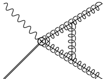
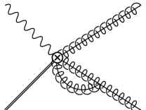
Figure 2: Diagrams needed to calculate the CS counterterm.

Diagrams involving usoft gluons vanish. Feynman rules for the vertex operators are given in Ref. FL . We perform our calculation in Feynman gauge, and obtain a relatively simple result for the one-loop UV-divergent term

$${\cal A} = \frac{1}{\epsilon}\,\sum_{\omega}{\cal O}(1,{}^{3}S_{1})(\omega)\frac{\alpha_{s}(\mu)C_{A}}{2\pi}\bigg{[}1$$

$$+\frac{M^{2}+\omega^{2}}{M^{2}}\bigg{(}\frac{M}{M+\omega}\ln\frac{M-\omega}{2M}+\frac{M}{M-\omega}\ln\frac{M+\omega}{2M}\bigg{)}\bigg{]}.$$

This depends on the large momentum component of the gluons. The divergent piece must be canceled by the counterterm $Z_{3}/Z_{\cal O}-1$, where $Z_{\cal O}$ is the CS vertex counterterm, and $Z_{3}$ is the gluon wavefunction counterterm

$$Z_{3}=1+\frac{\alpha_{s}}{4\pi}\frac{1}{\epsilon}\left(C_{A}\frac{5}{3}-n_{f}\frac{2}{3}\right)\,.$$ (27)

The anomalous dimension is obtained through the standard method, and the RGE for the coefficient is

$$\mu\frac{d}{d\mu}\Gamma^{(1,{}^{3}S_{1})}(\mu,\omega)=\gamma(\mu,\omega)\Gamma^{(1,{}^{3}S_{1})}(\mu,\omega)\,.$$ (28)

Solving this equation gives

$$\ln\!\bigg{(}\frac{\Gamma^{(1,{}^{3}S_{1})}(\mu,\omega)}{\Gamma^{(1,{}^{3}S_{1})}(M,\omega)}\bigg{)} =$$

$$\frac{2}{\beta_{0}}\bigg{\{}C_{A}\bigg{[}\frac{11}{6}+\frac{M^{2}+\omega^{2}}{M^{2}}\bigg{(}\frac{M}{M+\omega}\ln\frac{M-\omega}{2M}$$

$$+\frac{M}{M-\omega}\ln\frac{M+\omega}{2M}\bigg{)}\bigg{]}-\frac{n_{f}}{3}\bigg{\}}\ln\!\bigg{(}\frac{\alpha_{s}(\mu)}{\alpha_{s}(M)}\bigg{)}.$$

Logarithms of the form $\ln(\mu/M)$ have been summed into $\Gamma^{(1,{}^{3}S_{1})}(\mu,\omega)$, and any logarithms in the operator are of the form $\ln(\mu_{c}/\mu)$. If we take $\mu\sim\mu_{c}$ all large logarithms of the ratio $\mu_{c}/M$ will sit in the coefficient.

We now obtain the resummed rate, by substituting Eq. (The Resummed Photon Spectrum in Radiative $\Upsilon$ Decays) into Eq. (23), giving

$${\rm Im}T(z) = 2M\int d\ell^{+}\,S(\ell^{+})\,\Theta[\ell^{+}+M(1-z)]$$

$$\times\frac{16\pi}{3}\bigg{(}\frac{4\alpha_{s}(M)ee_{b}}{3M^{2}}\bigg{)}^{2}\int_{0}^{1}d\eta\bigg{[}\frac{\alpha_{s}(M\sqrt{1-z})}{\alpha_{s}(M)}\bigg{]}^{2\gamma(\eta)},$$

where $\eta=1/2(\xi+1)$ and

$$\gamma(\eta) \equiv \frac{2}{\beta_{0}}\bigg{\{}C_{A}\bigg{[}\frac{11}{6}$$

$$+\big{(}\eta^{2}+(1-\eta)^{2}\big{)}\bigg{(}\frac{1}{1-\eta}\ln\eta+\frac{1}{\eta}\ln(1-\eta)\bigg{)}\bigg{]}-\frac{n_{f}}{3}\bigg{\}}.$$

Again integrating over $\ell^{+}$ and inserting into Eq. (12), the resummed CS contribution to the decay rate is,

$$\frac{1}{\Gamma_{0}}\frac{d\Gamma_{\rm resum}}{dz}=z\int_{0}^{1}d\eta\bigg{[}\frac{\alpha_{s}(M\sqrt{1-z})}{\alpha_{s}(M)}\bigg{]}^{2\gamma(\eta)}.$$ (32)

We can expand in $\alpha_{s}(M)$ to obtain an analytic expression for the next-to-leading logarithmic contribution

$$\frac{1}{\Gamma_{0}}\frac{d\Gamma}{dz}=z\bigg{\{}1+\frac{\alpha_{s}}{6\pi}\big{[}C_{A}(2\pi^{2}-17)+2n_{f}\big{]}\ln(1-z)\bigg{\}}\,.$$ (33)

As $z$ approaches one the ${\cal O}(\alpha_{s})$ term becomes of order one, precisely the behavior observed in Ref. Kramer:1999bf . The resummed result does not suffer from this problem.

We now combine the different contributions to obtain a prediction for the photon spectrum. We will marry our expression for the CS spectrum in the endpoint with the leading order result by interpolating between the two

$$\frac{1}{\Gamma_{0}}\frac{d\Gamma_{\rm int}}{dz}=\bigg{(}\frac{1}{\Gamma_{0}}\frac{d\Gamma_{\rm LO}^{\rm dir}}{dz}-z\bigg{)}+\frac{1}{\Gamma_{0}}\frac{d\Gamma_{\rm resum}}{dz}\,.$$ (34)

Before we proceed we need the NRQCD MEs. We can extract the CS ME from the $\Upsilon$ leptonic width. The CO MEs are more difficult to determine. NRQCD predicts that the CO MEs scale as $v^{4}$ compared to the CS ME. In Ref. Petrelli:1998ge it was argued that an extra factor of $1/2N_{c}$ should be included. We set the ${}^{1}S_{0}$ and ${}^{3}P_{0}$ MEs to zero, and the ${}^{3}S_{1}$ ME to $\langle\Upsilon|{\cal O}_{8}(^{3}S_{1})|\Upsilon\rangle=v^{4}\langle\Upsilon|{\cal O}_{1}(^{3}S_{1})|\Upsilon\rangle$, where we use $v^{2}=0.08$.

The CLEO collaboration measured the number of photons in inclusive $\Upsilon(1S)$ radiative decays Nemati:1996xy . The data does not remove the efficiency or energy resolution and is the number of photons in the fiducial region, $|\cos\theta|<0.7$. In order to compare our theoretical prediction to the data, we integrate over the barrel region and convolute with the efficiency that was modeled in the CLEO paper. We do not do a bin-to-bin smearing of our prediction.

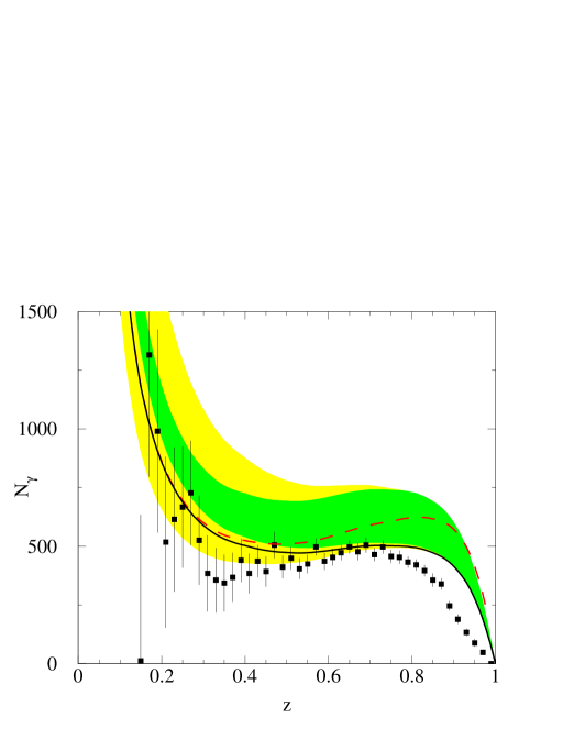
Figure 3: The inclusive photon spectrum, compared with data Nemati:1996xy . The theory predictions are described in the text.

In Fig. 3 we compare our prediction to the data. The error bars on the data are statistical only. The dashed line is the direct tree-level plus fragmentation result, while the solid curve includes the resummation in Eq. (34). For these two curves we use the $\alpha_{s}$ extracted from these data, $\alpha_{s}(M_{\Upsilon})=0.163$, which corresponds to $\alpha_{s}(M_{Z})=0.110$ Nemati:1996xy . The shape of the resummed result is much closer to the data than the tree-level curve, though it is not a perfect fit. We also show the Eq. (34) plus fragmentation result, using the PDG value of $\alpha_{s}(M_{Z})$, including theoretical uncertainties, denoted by the shaded region. To obtain the darker band, we first varied the choice of $m_{b}$ between $4.7{\rm\ GeV}<m_{b}<4.9{\rm\ GeV}$ and the value of $\alpha_{s}$ within the errors given in the PDG, $\alpha_{s}(M_{Z})=0.1172(20)$ Hagiwara:pw . Varying $m_{b}$ and $\alpha_{s}$ modifies the extraction of the CS ME from $3.31{\rm\ GeV}^{3}$ to $3.56{\rm\ GeV}^{3}$. We also varied the collinear scale, $\mu_{c}$ from $M\sqrt{(1-z)/2}<\mu_{c}<M\sqrt{2(1-z)}$. Finally, the lighter band also includes the variation, within the errors, of the parameters for the quark to photon fragmentation function extracted by ALEPH Buskulic:1995au . The low $z$ prediction is dominated by the quark to photon fragmentation coming from the CO ${}^{3}S_{1}$ channel. We did not assign any error to the CO ${}^{3}S_{1}$ ME. Since it is unknown, there is a very large uncertainty in the lower part of the prediction that we decided not to show. Note that the CO ${}^{1}S_{0}$ and ${}^{3}P_{0}$ contribution increases the theoretical prediction at the upper endpoint FL . It is thus clear the data favors a very small value for the CO ${}^{1}S_{0}$ and ${}^{3}P_{0}$ MEs. This is why we set these to zero in our analysis. Negative values for these MEs are possible, and would give a bit better fit to the shape.

References

• (1) S. J. Brodsky et al., Phys. Lett. B 73, 203 (1978); K. Koller and T. Walsh, Nucl. Phys. B 140, 449 (1978).
• (2) G. T. Bodwin et al., Phys. Rev. D 51, 1125 (1995) [Erratum-ibid. D 55, 5853 (1995)]; M. E. Luke et al., Phys. Rev. D 61, 074025 (2000).
• (3) S. Catani and F. Hautmann, Nucl. Phys. Proc. Suppl.  39BC, 359 (1995).
• (4) F. Maltoni and A. Petrelli, Phys. Rev. D 59, 074006 (1999).
• (5) I. Z. Rothstein and M. B. Wise, Phys. Lett. B 402, 346 (1997).
• (6) C. W. Bauer et al., Phys. Rev. D 64, 114014 (2001).
• (7) M. Kramer, Phys. Rev. D 60, 111503 (1999).
• (8) B. Nemati et al. [CLEO Collaboration], Phys. Rev. D 55, 5273 (1997).
• (9) C. W. Bauer et al., Phys. Rev. D 63, 014006 (2001); C. W. Bauer et al., Phys. Rev. D 63, 114020 (2001).
• (10) C. W. Bauer and I. W. Stewart, Phys. Lett. B 516, 134 (2001); C. W. Bauer et al., Phys. Rev. D 65, 054022 (2002).
• (11) S. Fleming and A. K. Leibovich, work in progress.
• (12) C. W. Bauer et al., Phys. Rev. D 66, 014017 (2002).
• (13) A. Petrelli et al., Nucl. Phys. B 514, 245 (1998).
• (14) K. Hagiwara et al. [Particle Data Group Collaboration], Phys. Rev. D 66, 010001 (2002).
• (15) D. Buskulic et al. [ALEPH Collaboration], Z. Phys. C 69, 365 (1996).