QCD EVOLUTION OF TRANSVERSITY
IN LEADING AND NEXT-TO-LEADING ORDER

Abstract

I shall present a rather pedagogical discussion of the transversity distributions in the quark-parton model and, in particular, the rôle of perturbative ?QCD? corrections. Among the topics I shall discuss are: ?LO? and ?NLO? evolution, the Soffer bound and so-called $K$ factors in the Drell–Yan process. The main conclusion will be that, compared to unpolarised or even longitudinally polarised hadron scattering, the case of transverse spin should actually provide a far clearer window onto the workings of ?QCD? and the interplay with the ?QPM?.

1 Introduction

1.1 Overview of the talk

In the past there has been the rather damning prejudice that all transverse-spin effects (if not indeed spin effects tout court) should vanish at very high energies (i.e., where mass effects may be neglected). This has led to a general lack of interest in the subject on both the experimental and theoretical sides, with some notable exceptions. This is now known not to be the case.

Indeed, in the near future (and already to some extent) the interest at the level of the ?QPM? (?QPM?)?QPM? in generic deeply-inelastic hadron scattering is due to shift from unpolarised (and even longitudinally polarised) hadrons to transversely polarised states. While, on the one hand, the first natural question to ask is simply the magnitude of the relevant partonic densities, on the other (however, intimately related), there is the problem of evolution and the general framework of perturbative ?QCD? (?QCD?)?QCD?.

A schematic overview of this talk is then as follows:

• brief history and notation

• operator-product expansion and renormalisation group

• ?QCD? evolution

  • leading order

  • next-to-leading order

  • effects on asymmetries

  • effects on the Soffer bound

• a ?DIS? definition

• ?DIS?–?DY? $K$ factor

• comments and concluding remarks

1.2 A brief history of transversity

The history of transversity (the concept though not the precise terminology) begins as early as 1979 with its introduction by Ralston and Soper [1] via the Drell–Yan process. Shortly following this the ?LO? (?LO?)?LO? anomalous dimensions were first calculated by Baldracchini et al. [2] and …promptly forgotten! This decided lack of interest may be partly traced to the inaccessibility of transversity via the archetypal parton-model process: namely, ?DIS? (?DIS?)?DIS?. Indeed, as we shall see, the typical process in which transversity may be measured involves at least two polarised hadrons.

A further obstacle was created by the common theoretical prejudice, already mentioned, according to which precisely transverse-spin effects (i.e., asymmetries) should actually vanish at high energies. The reasons for such a belief lie in the requirement of chirality-flip in the relevant amplitudes, a property not enjoyed under typical circumstances by a theory of nearly massless fermions interacting via gauge bosons; however, as shown by Ralston and Soper [1], it turns out that there are indeed several (otherwise standard) processes in which such effects are on a par with the unpolarised and helicity-weighted cross-sections.

During the period of great revival witnessed by the spin community, following the EMC revelations regarding the proton spin, the ?LO? anomalous dimensions for transversity distributions were recalculated by Artru and Mekhfi [3]. It is worth recalling that, in fact, these calculations had also already been, so to speak, unwittingly performed (as contributions to the evolution of the ?DIS? structure function $g_{2}$) by: Kodaira et al. [4], Antoniadis and Kounnas [5], Bukhvostov, Kuraev and Lipatov [6], and Ratcliffe [7].

With the typical precision of modern ?DIS? measurements, a complete knowledge of the radiative corrections up to ?NLO? (?NLO?)?NLO? is indispensable; in the case of transversity the ?NLO? anomalous dimensions were calculated by: Hayashigaki, Kanazawa and Koike [8], Kumano and Miyama [9], and Vogelsang [10]. Armed with results of such calculations, it is then possible to proceed with an examination of the phenomenological effects of ?QCD? evolution: studies have been performed by a number of authors; the interested reader is referred to a recent review paper by Barone, Drago and Ratcliffe, where indeed more details of much of what follows may be found. The lectures by Jaffe [12] also provide a useful pedagogical presentation while an important early technical discussion laying down the ground rules was given by Jaffe and Ji [13].

1.3 Notation

Unfortunately, owing to the somewhat sparse theoretical effort, the literature now abounds with conflicting notation in regard of the transversity distributions. For a list and discussion, see Ref. [11], in accordance with which I shall adopt the form $\Delta_{T}{f}$ to indicate the transverse-spin weighted quark density:

$$\Delta_{T}{f}(x)=f_{\uparrow}(x)-f_{\downarrow}(x)\,,$$ (1)

where $f_{\uparrow,\downarrow}(x)$ indicates a parton of type $f$ with transverse spin vector $\uparrow$ parallel or antiparallel to that of the parent hadron.

At this point it is worth underlining the fact that while one normally talks of partonic densities and ?DIS? structure functions completely interchangeably, in the case of transversity there no ?DIS? structure function. Thus, any reference to $h_{1}$ should only be taken as a generic indication of transversity dependence, with no particular relation to ?DIS?.

2 Technical Basis

2.1 Transverse spin projectors

Since we are necessarily dealing with transverse spin, it is useful to define the corresponding polarisation projectors. The transverse polarisation projectors along the $x$ and $y$ directions (motion is always understood to be along the $z$-axis) are

$$\begin{split}\mathcal{P}_{\uparrow\downarrow}^{(x)}&={\textstyle\frac{1}{2}}\,(1\pm\gamma^{1}\gamma_{5})\,,\\ \mathcal{P}_{\uparrow\downarrow}^{(y)}&={\textstyle\frac{1}{2}}\,(1\pm\gamma^{2}\gamma_{5})\,,\end{split}$$ (2)

for positive-energy states and

$$\begin{split}\mathcal{P}_{\uparrow\downarrow}^{(x)}&={\textstyle\frac{1}{2}}\,(1\mp\gamma^{1}\gamma_{5})\,,\\ \mathcal{P}_{\uparrow\downarrow}^{(y)}&={\textstyle\frac{1}{2}}\,(1\mp\gamma^{2}\gamma_{5})\,,\end{split}$$ (3)

for negative-energy states

2.2 Basis states and amplitudes

A transversity or transverse-spin basis (with the spin vector $\uparrow$ directed along $y$, for instance) may be expressed in terms of the more familiar helicity states as

$$\begin{array}[]{lcr}\left|\uparrow\right\rangle&=&\frac{1}{\sqrt{\vphantom{0}}2}\left[\,\left|+\right\rangle+\I\left|-\right\rangle\right],\\[4.30554pt] \left|\downarrow\right\rangle&=&\frac{1}{\sqrt{\vphantom{0}}2}\left[\,\left|+\right\rangle-\I\left|-\right\rangle\right].\end{array}$$ (4)

The transverse polarisation distributions $\Delta_{T}{f}$ is then related to an amplitude that is diagonal in transverse-spin space, while in an helicity base it is described as an interference effect:

$$\Delta_{T}{f}(x)=f_{\uparrow}(x)-f_{\downarrow}(x)\sim\mathop{\text{Im}}\nolimits\mathcal{A}_{+-,-+}\,.$$ (5)

2.3 Chirality flip

That helicity (or chirality—the terms coincide for massless states) is flipped in the amplitudes involved is represented pictorially in Fig. 1:

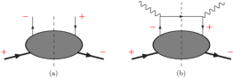
Figure 1: (a) A chirally-odd hadron–quark amplitude for the $h_{1}$ partonic density. (b) The chirality-flip forbidden ?DIS? handbag diagram.

The chirally-odd hadron–quark amplitude contributing to a would-be ?DIS? transversity structure function $h_{1}$ is depicted in Fig. 1a. However, the full ?DIS? handbag diagram shown in Fig. 1b demonstrates the absence of such a structure owing to the presence of massless propagators and to helicity conservation at the vector vertices (typical of gauge theories such as QED and ?QCD?). Note, however, that chirality flip is not a problem if the quark lines of opposite chirality connect to different hadrons, as for example in the ?DY? (?DY?)?DY? process.

2.4 Twist basics and operators

Let us now place transversity in its proper context, together with the better known spin-averaged and helicity-weighted parton densities. Note, of course, although we have just seen that a transversity contribution to fully inclusive ?DIS? is precluded, this is merely due to the nature of that particular process and not to any fundamental suppression or absence of transversity itself. Thus, it is more useful to simply consider the corresponding partonic densities.

Transversity is one of the three leading-twist (twist-two) structures:

$$f(x) = \int\!\frac{\D\xi^{-}}{4\pi}\;\E^{\I xP^{+}\xi^{-}}\left\langle PS\right|\mathchoice{\makebox[0.0pt][l]{$\displaystyle\kern 2.08334pt\overline{\kern-2.43059pt\phantom{\psi}}$}}{\makebox[0.0pt][l]{$\textstyle\kern 2.08334pt\overline{\kern-2.43059pt\phantom{\psi}}$}}{\makebox[0.0pt][l]{$\scriptstyle\kern 1.45834pt\overline{\kern-1.7014pt\phantom{\psi}}$}}{\makebox[0.0pt][l]{$\scriptscriptstyle\kern 1.04167pt\overline{\kern-1.21529pt\phantom{\psi}}$}}\psi(0)\gamma^{+}\psi(0,\xi^{-},\mathchoice{\mbox{\boldmath$\displaystyle 0$\unboldmath}}{\mbox{\boldmath$\textstyle 0$\unboldmath}}{\mbox{\boldmath$\scriptstyle 0$\unboldmath}}{\mbox{\boldmath$\scriptscriptstyle 0$\unboldmath}}_{\perp})\left|PS\right\rangle\,,$$ (6)

$$\Delta{f}(x) = \int\!\frac{\D\xi^{-}}{4\pi}\;\E^{\I xP^{+}\xi^{-}}\left\langle PS\right|\mathchoice{\makebox[0.0pt][l]{$\displaystyle\kern 2.08334pt\overline{\kern-2.43059pt\phantom{\psi}}$}}{\makebox[0.0pt][l]{$\textstyle\kern 2.08334pt\overline{\kern-2.43059pt\phantom{\psi}}$}}{\makebox[0.0pt][l]{$\scriptstyle\kern 1.45834pt\overline{\kern-1.7014pt\phantom{\psi}}$}}{\makebox[0.0pt][l]{$\scriptscriptstyle\kern 1.04167pt\overline{\kern-1.21529pt\phantom{\psi}}$}}\psi(0)\gamma^{+}\gamma_{5}\psi(0,\xi^{-},\mathchoice{\mbox{\boldmath$\displaystyle 0$\unboldmath}}{\mbox{\boldmath$\textstyle 0$\unboldmath}}{\mbox{\boldmath$\scriptstyle 0$\unboldmath}}{\mbox{\boldmath$\scriptscriptstyle 0$\unboldmath}}_{\perp})\left|PS\right\rangle\,,$$ (7)

$$\Delta_{T}{f}(x) = \int\!\frac{\D\xi^{-}}{4\pi}\;\E^{\I xP^{+}\xi^{-}}\left\langle PS\right|\mathchoice{\makebox[0.0pt][l]{$\displaystyle\kern 2.08334pt\overline{\kern-2.43059pt\phantom{\psi}}$}}{\makebox[0.0pt][l]{$\textstyle\kern 2.08334pt\overline{\kern-2.43059pt\phantom{\psi}}$}}{\makebox[0.0pt][l]{$\scriptstyle\kern 1.45834pt\overline{\kern-1.7014pt\phantom{\psi}}$}}{\makebox[0.0pt][l]{$\scriptscriptstyle\kern 1.04167pt\overline{\kern-1.21529pt\phantom{\psi}}$}}\psi(0)\gamma^{+}\gamma^{1}\gamma_{5}\psi(0,\xi^{-},\mathchoice{\mbox{\boldmath$\displaystyle 0$\unboldmath}}{\mbox{\boldmath$\textstyle 0$\unboldmath}}{\mbox{\boldmath$\scriptstyle 0$\unboldmath}}{\mbox{\boldmath$\scriptscriptstyle 0$\unboldmath}}_{\perp})\left|PS\right\rangle\,,$$ (8)

where the state $\left|PS\right\rangle$ represents a baryon of four-momentum $P$ and spin four-vector $S$. The $\gamma_{5}$ matrix appearing in the second and third lines signals spin dependence while the extra $\gamma^{1}$ matrix in $\Delta_{T}{f}(x)$ signals the helicity-flip that precludes transversity contributions in ?DIS?.

2.5 Gluon transversity

Before continuing with a discussion of the quark case, it is worth noting that transversity may also exist for gluons: it corresponds to linearly polarised states in a transversely polarised hadron. However, conventional wisdom has it that, owing to $t$-channel helicity conservation, a spin-half baryon cannot support the two units of spin-flip necessary for gluon transversity and thus one is led to the perhaps somewhat surprising conclusion that gluons may not be transversely polarised inside transversely polarised baryons!

Now, I should point out that such an argument does not take into account orbital-angular momentum! Let me simply recall that the ?AP? (?AP?)?AP? kernels inevitably generate orbital-angular momentum [15]; thus it might be that gluon transversity can be generated in a composite object such as a baryon; no calculations to such effect exist though. This problem apart, it is certainly true, as we shall see shortly, that the quark and gluon transversity densities evolve independently. This fact alone renders transversity an interesting case for evolution studies—the subject to which I now turn.

2.6 The ?OPE? and ?RGE?

The ?OPE?, as applied to ?DIS?, is illustrated pictorially in Fig. 2.

handbag0 (40,30) thick i1,i2 o1,o2 fermion,tension=0.5i1,v1 fermion,tension=0.5v1,v2 fermion,tension=0.5v2,o1 photoni2,v1 photonv2,o2  =  $\displaystyle\sum_{n}C_{n}$ operator0 (20,30) thick i1,o1 v1 fermion,tension=0.5i1,v1 fermion,tension=0.5v1,o1 decor.shape=circle,decor.filled=empty,decor.size=10v1

Figure 2: A pictorial representation of the ?OPE? as applied to ?DIS?.

The anomalous dimensions, $\gamma_{n}$, are then obtained from the logarithmic terms in the loop corrections to the right-hand side (i.e., the renormalisation of the operators ${O}_{n}$) while the Wilson coefficients, $C_{n}$, receive corrections calculated from the loop corrections to the left-hand side (i.e., the renormalisation of the hard-scattering cross-section $\hat{\sigma}$). The so-formed ?RGE? (?RGE?)?RGE? takes the form

$$\frac{\partial{{O}_{n}}(\mu^{2})}{\partial\ln\mu^{2}}+\gamma_{n}\left(\alpha_{s}(\mu^{2})\right){O}_{n}(\mu^{2})=0\,,$$ (9)

with standard formal solution

$${O}_{n}(Q^{2})={O}_{n}(\mu^{2})\,\exp\left[-\int_{\alpha_{s}(\mu^{2})}^{\alpha_{s}(Q^{2})}\!\D{\alpha_{s}}\frac{{\gamma_{n}}(\alpha_{s})}{\beta(\alpha_{s})}\right].$$ (10)

2.7 Ladder diagram summation

It is instructive to examine the question of evolution within the framework of the ladder-diagram summation technique [18, 19]. Recall that the principal tool of this approach is the use of a physical (axial or light-like) gauge, in which none but the ladder (planar) diagrams survive the requirement of a large logarithm. In such a gauge the one-loop ?AP? ?OPI? (?OPI?)?OPI? kernels for the leading-twist structures are given by the diagram shown in Fig. 3.

gluonrung1 (40,30) thick curly_len3mm i1,o2 o1,i2 fermion,label=$+$,l.side=lefti1,v1 fermion,label=$+$,l.side=leftv1,o1 fermion,label=$-$,l.side=lefti2,v2 fermion,label=$-$,l.side=leftv2,o2 gluonv1,v2

Figure 3: The ?OPI? universal kernel in a physical (axial) gauge governing the ?QCD? evolution of the partonic transversity distributions.

In the case of transversity the diagram has a different helicity structure to those of the spin-averaged and helicity-weighted cases and thus, not surprisingly, the anomalous dimensions are different in this case.

Consider now one of the ?OPI? kernels to be calculated for the full flavour-singlet evolution and that would mix quark and gluon contributions, as shown in Fig. 4.

fermionrung1 (40,30) thick i1,o2 o1,i2 fermioni1,v1 gluonv1,o1 gluoni2,v2 fermionv2,o2 fermion,label=$+$,l.side=lefti1,v1 fermion,label=$-$,l.side=leftv2,o2 fermion,label=?v1,v2

Figure 4: The disallowed ?OPI? kernel that would mix the quark and gluon contributions to transversity were it not for helicity conservation at the vertices.

Once again the helicity-conserving nature of gauge theories in the massless (or high-energy) limit leads to a peculiarity in the case of transversity: ?LO? ?QCD? evolution of transversity is non-singlet like. Thus, even where a gluon transversity may exist (e.g., in the deuteron) there is no mixing between the flavour-singlet quark and gluon transversity densities: the two evolve independently. This means that, for example, for equal statistical precision, the experimental study of transversity evolution would provide a far better evaluation of, say, $\alpha_{s}$; recall that in the spin-averaged and too in the helicity-weighted cases the strong correlation between $\alpha_{s}$ and the ill-determined gluon distributions drastically reduces the significance of the extracted value of $\alpha_{s}$. Note also that the usually quoted ?DIS? values for $\alpha_{s}$ essentially come from sum-rule measurements and thus from Wilson coefficient corrections and not evolution.

2.8 Interpolating currents

It is also interesting to examine the problem via a method suggested by Ioffe and Khodjamirian [20]. The idea is simply to use a pair of interpolating currents that have the correct chirality structure—in this case one vector and one scalar, with the scalar providing the necessary spin-flip, see Fig. 5.

higgs0 (40,30) thick i1,i2 o1,o2 fermion,tension=0.5,label=$+$,l.side=lefti1,v1 fermion,tension=0.5,label=$+$,l.side=leftv1,v2 fermion,tension=0.5,label=$-$,l.side=leftv2,o1 photoni2,v1 scalarv2,o2

Figure 5: A hypothetical Higgs–photon interference term that could contribute to the ?DIS? cross-section in the case of a transversely polarised hadron.

The anomalous dimensions are then obtained from the leading logarithmic corrections to the diagram in Fig. 4. A first attempt at calculating $\gamma_{n}$ with this method gave an apparently contradictory result—subsequently corrected by Blümlein [21]. The critical observation is that while the vector current $J_{V}$ is conserved and therefore has $\gamma_{V}=0$, the scalar current $J_{S}$ is not conserved and thus has $\gamma_{S}{\hbox{}\not=\hbox{}}0$.

Now, the product of two currents may be expanded as

$$J_{V}(z)\cdot J_{S}(0)=\sum_{n}\,C(n;z)\,{O}(n;0)\,,$$ (11)

and the ?RGE? for the Wilson coefficients $C(n;z)$ is

$$\left[\mathcal{D}+\gamma_{J_{V}}(g)+\gamma_{J_{S}}(g)-\gamma_{{O}}(n;g)\rule[-4.30554pt]{0.0pt}{12.91663pt}\right]C(n;z)=0\,,$$ (12)

where the ?RG? (?RG?)?RG? operator is

$$\mathcal{D}=\mu^{2}\frac{\partial}{\partial\mu^{2}}+\beta(g)\frac{\partial}{\partial{g}}\,.$$ (13)

Therefore, this chirally-odd interference version of the “Compton” amplitude correction has renormalisation coefficient

$$\gamma_{C}(n;g)=\gamma_{J_{V}}(g)+\gamma_{J_{S}}(g)-\gamma_{{O}}(n;g)\,.$$ (14)

As explained above, while $\gamma_{J_{V}}=0$ (corresponding to the conservation of the vector current), $\gamma_{J_{S}}\not=0$ (the scalar current is not conserved).

We shall discuss later on how this approach suggests a method of examining the possible $K$ factors involved in the corresponding ?DY? process.

3 ?QCD? Evolution

First, let us now examine a little more thoroughly the evolution problem in ?QCD?, with particular attention to the case of transversity. I shall discuss the ?LO? results in some detail and then simply limit myself to a demonstration of the effect of including ?NLO? corrections.

3.1 Leading order quark–quark kernels

The well-known results for the ?LO? (indicated by the $0$ index below) ?AP? quark–quark splitting functions in the three twist-two cases are:

$$P_{qq}^{(0)} = C_{\text{F}}\left(\frac{1+x^{2}}{1-x}\right)_{+}\,,$$ (15)

$$\Delta{P}_{qq}^{(0)} = P_{qq}^{(0)}\quad\mbox{helicity conservation,}$$ (16)

$$\Delta_{T}{P}_{qq}^{(0)} = C_{\text{F}}\left[\left(\frac{1+x^{2}}{1-x}\right)_{+}-1+x\right]$$ (17)

$$= P_{qq}^{(0)}(x)-C_{\text{F}}(1-x)\,.$$ (18)

It is useful to define Mellin moments of all quantities involved (partonic densities, splitting kernels and Wilson coefficients):

$$f^{(n)}\equiv\int_{0}^{1}\D{x}\,x^{n-1}\,f(x)\,.$$ (19)

The first moments (i.e., with $n=1$) of the partonic densities often correspond to sum rules (deriving from conserved quantities or symmetries), which may be determined independently by other experimental measurements.

Note that for both $P_{qq}^{(0)}$ and $\Delta{P}_{qq}^{(0)}$ the first moments vanish (a consequence of vector and axial-vector conservation implying the existence of sum rules corresponding, e.g., to the total charge and the neutron beta-decay axial coupling $g_{A}$) while for $\Delta_{T}{P}_{qq}^{(0)}$ the same is not true and the sign implies a falling first moment (the so-called tensor charge) for transversity. While such a suppression of transversity has obvious negative implications for high-energy measurements in terms of the size of effect (asymmetry) one might hope to measure, it does also indicate a more rapid evolution than in the other two leading-twist cases. This, coupled to the independence from the gluon density, would imply a greater sensitivity to, for example, the value of $\alpha_{s}$.

3.2 Leading order gluon–gluon kernels

For completeness, let us now briefly list the corresponding results for the purely gluonic sector. The three ?DGLAP? (?DGLAP?)?DGLAP? gluon–gluon splitting functions at ?LO? are as follows:

$$P_{gg}^{(0)} = C_{\text{G}}\left[\frac{2x}{(1-x)_{+}}+2x(1-x)+\frac{2(1-x)}{x}\right]$$ (20)

$$\hskip 65.00009pt\hbox{}+\left[\frac{11}{6}C_{\text{G}}-\frac{2}{3}T_{\text{F}}\right]\,\delta(x-1)\,,$$

$$\Delta{P}_{gg}^{(0)} = C_{\text{G}}\left[\frac{2x}{(1-x)_{+}}+4(1-x)\right]$$ (21)

$$\hskip 65.00009pt\hbox{}+\left[\frac{11}{6}C_{\text{G}}-\frac{2}{3}T_{\text{F}}\right]\,\delta(x-1)\,,$$

$$\Delta_{T}{P}_{gg}^{(0)} = C_{\text{G}}\left[\frac{2x}{(1-x)_{+}}\right]+\left[\frac{11}{6}C_{\text{G}}-\frac{2}{3}T_{\text{F}}\right]\,\delta(x-1)\,.$$ (22)

The first moment in the helicity case, is precisely the leading-order $\beta$-function coefficient $\beta_{0}$. Thus, the first moment of the helicity density $\Delta{g}$ grows as $1/\alpha_{s}$, for the transversity density case $\Delta_{T}{g}$ grows less, while $g$ (which, of course, is actually infinite) grows more (as $1/x$). All three kernels behave similarly for $x\to 1$.

3.3 Orbital angular momentum

It is also natural to ask how the question of orbital angular momentum develops in the case of transversity. Now, since $\Delta_{T}{q}$ and $\Delta_{T}{g}$ evolve independently (recall there is no mixing), the total spin fraction of each of the two parton types must be conserved separately. Thus, in the usual way, the splitting functions necessarily generate compensating orbital angular momentum, but for each separately.

Given that $\Delta_{T}{q}$ decreases with increasing $Q^{2}$, $L_{T}^{q}$ must increase in magnitude (assuming a “primordial” value of zero) with the same sign as the initial quark spin; the final value will however be limited. In contrast, $\Delta_{T}{g}$ increases without bound (just as $\Delta{g}$); thus, $L_{T}^{g}$ must also increase in magnitude, but with the opposite sign to the initial gluon spin.

3.4 ?LO? evolution

The physical implications of evolution for the transversity distributions may now be examined. Obviously, still lacking is a starting distribution: a reasonable model may be provided by taking $\Delta_{T}{q}=\Delta{q}$ at some very low scale. The ?LO? evolution for such a hypothetical $u$-quark distribution is displayed in Fig. 6.

Figure 6: The evolution of $u$-quark helicity and transversity distributions compared. The input is $\Delta_{T}{u}=\Delta{u}$ at $Q_{0}^{2}=0.23\,\text{GeV}^{2}$ (dashed curve). The solid (dotted) curve shows $\Delta_{T}{u}$ ($\Delta{u}$) at $Q^{2}=25\,\text{GeV}^{2}$. The dot–dashed curve shows the non-singlet evolution of $\Delta_{T}{u}$ at $Q^{2}=25\,\text{GeV}^{2}$ driven by $P_{qq}$.

The relative weakening of the transversity distribution with increasing scale is evident. The top (dot–dashed) curve shows the evolution of $\Delta_{T}{u}$ obtained using $P_{qq}$ (in place of $\Delta_{T}{P}_{qq}$), the difference with respect to the standard evolution of $\Delta{u}$ is due entirely to the lack (presence) of gluon mixing in the the transversity (helicity) case.

3.5 Next-to-leading order kernels

As we move to ?NLO? the situation becomes a little more complicated: while there is still no quark–gluon mixing (for the same reasons), there does arise quark–antiquark mixing due to pair production (as is usual at this order). In addition, of course, the expressions get much longer and harder to calculate! The calculations have been performed by three groups: Hayashigaki, Kanazawa and Koike [8], Kumano and Miyama [9], and Vogelsang [10]. In addition, the gluon case has been dealt with by Vogelsang [25].

The one-loop coefficient functions for ?DY? are also known, and in different renormalisation schemes, see Vogelsang and Weber [26], Contogouris, Kamal and Merebashvili [27], Kamal [28], and Vogelsang [10]. However, such corrections are not yet known for any other process.

3.6 ?NLO? evolution

The full ?NLO? evolution may thus be studied phenomenologically. Again not having any data input for $\Delta_{T}{q}_{qq}$ we must resort to modelling, typically by assuming equality with the helicity distributions at some starting scale. The effects of ?NLO? evolution on the first two moments are displayed in Fig. 7;

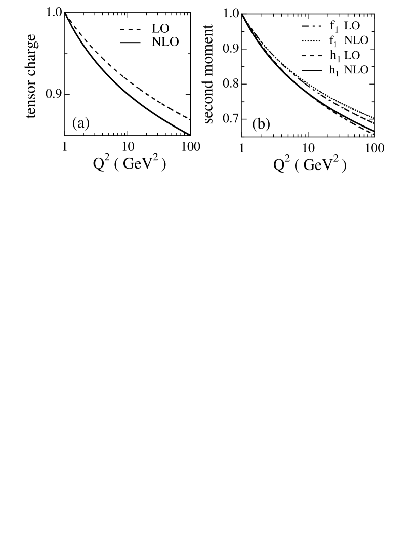
Figure 7: The ?LO? and ?NLO? $Q^{2}$-evolution of (a) the tensor charge and (b) the second moments of $h_{1}(x,Q^{2})$ and $f_{1}(x,Q^{2})$, all curves are normalised to unity at $Q^{2}=1\,\text{GeV}^{2}$ (taken from [8]).

recall that the vector and axial-vector charges are constant. In Fig. 8

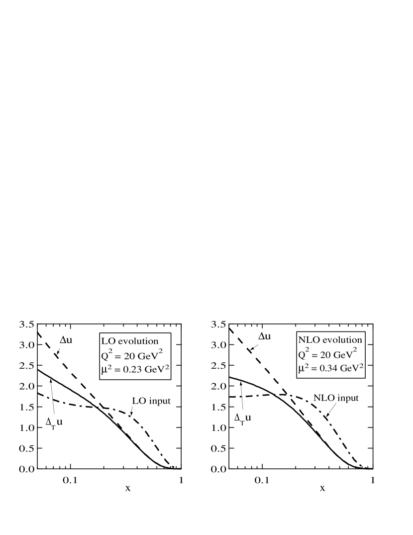
(a)                                                     (b)

Figure 8: A comparison of the $Q^{2}$-evolution of $\Delta_{T}{u}(x,Q^{2})$ and $\Delta{u}(x,Q^{2})$ at (a) ?LO? and (b) ?NLO?, assuming the same starting values as input (taken from [8]).

a comparison is shown of the effects at ?LO? and ?NLO?. Note that there is also a difference in the input moving from ?LO? to ?NLO? owing to the differing Wilson coefficients at ?NLO?.

4 The Soffer Bound

In the case of spin-dependent distributions there exist rather obvious positivity bounds with respect to the corresponding unpolarised cases: since the $q_{\pm}$ are positive definite (at least in the naïve parton model) it follows that $|\Delta{q}|\leq{q}$ (the former being the difference and the latter the sum of the same two positive definite quantities), with an analogous inequality also holding for $|\Delta_{T}{q}|$. In addition, the transversity distribution is constrained by a much less obvious bound derived by Soffer [29]. The derivation, which we shall follow somewhat schematically, is an instructive example of the necessity of considering amplitudes and not simple probability densities when dealing with problems involving spin states. The central point here is the presence of both longitudinal and transverse spin states; thus either one or the other must be translated into a different basis.

It is useful to introduce the following hadron–parton amplitudes:

in terms of which the various partonic densities may be expressed as various combinations,

$$f(x) \propto\mathop{\text{Im}}\nolimits(\mathcal{A}_{++,++}+\mathcal{A}_{+-,+-}) \propto\sum_{X}(a_{++}^{*}a_{++}+a_{+-}^{*}a_{+-})\,,$$ (23)

$$\Delta{f}(x) \propto\mathop{\text{Im}}\nolimits(\mathcal{A}_{++,++}-\mathcal{A}_{+-,+-}) \propto\sum_{X}(a_{++}^{*}a_{++}-a_{+-}^{*}a_{+-})\,,$$ (24)

$$\Delta_{T}{f}(x) \propto\mathop{\text{Im}}\nolimits\mathcal{A}_{+-,-+} \propto\sum_{X}a_{--}^{*}a_{++}\,.$$ (25)

Using these quantities it is then possible to construct a rather non-trivial Schwartz-type inequality:

$$\sum_{X}|a_{++}\pm a_{--}|^{2}\geq 0\quad\Rightarrow\quad\sum_{X}a_{++}^{*}a_{++}\pm\sum_{X}a_{--}^{*}a_{++}\geq 0\,,$$ (26)

which in turn leads to

$$f_{+}(x)\geq|\Delta_{T}{f}(x)|\quad\mbox{or}\quad f(x)+\Delta{f}(x)\geq 2|\Delta_{T}{f}(x)|\,.$$ (27)

This last inequality is precisely the Soffer bound, which interestingly involves all three leading-twist distributions. Such a bound can, of course, become particularly stringent in the case of helicity distributions that are negative, as is the case for the $d$ quark.

4.1 Evolution of the Soffer bound

The doubt immediately arises as to whether the bound is respected by ?QCD? evolution; this is not at all a futile question since it is well known that evolution (in particular, towards lower scales) does not even respect the basic positivity of the un-polarised densities. This problem can be traced to the fact that partonic densities are not physical quantities and thus beyond the ?LO? they are not well defined. A quark seen by a ?DIS? photon may be “primordial” in origin (in some definition) or be part of a $q\bar{q}$ pair created from a primordial gluon (in another). A redefinition of the densities may lead to a gluonic contribution to the physical ?DIS? cross-section exceeding the total cross-section. This will in turn determine a negative implied value for the primordial quark densities.

Now, the problem is different at ?LO? and ?NLO?. At leading order there are no ambiguities and one merely has to inspect the form of the ?AP? kernels. At ?NLO? there is no unique definition of the kernels and the situation is more complicated. Let us start by examining the situation at ?LO?. Maintenance of the Soffer bound under ?QCD? evolution has been argued by Bourrely, Leader and Teryaev [30]. It is indeed possible to make rather general arguments: the non-singular terms in the kernels are always positive definite and thus cannot affect positivity statements. However, the IR singular (“plus” regularised) terms in the kernel are negative and thus in principle can affect inequalities such as that of Soffer. Let us rewrite the plus-regularised terms in the following manner:

$$P_{+}(x,t)=P(x,t)-\delta(1-x)\int_{0}^{1}\frac{\D{y}}{y}\;P(y,t)\,.$$ (28)

The ?DGLAP? equations can then be recast in a Boltzmann form:

$$\frac{\D{q}(x,t)}{\D{t}}=\int_{x}^{1}\frac{\D{y}}{y}\;q(y,t)\,P\!\left(\frac{x}{y},t\right)-\int_{0}^{x}\frac{\D{y}}{x}\;q(x,t)\,P\!\left(\frac{y}{x},t\right).$$ (29)

One sees that the negative term on the right-hand side is “diagonal” in $x$ and thus cannot change the sign of $q(x,t)$, since $q(x,t)$ must go through zero to turn negative, at which point the evolution switches off. Thus, let us write

$$\frac{\D{q}_{\pm}(x,t)}{\D{t}}=P_{+\pm}(x,t)\otimes q_{+}(x,t)+P_{+\mp}(x,t)\otimes q_{-}(x,t)\,.$$ (30)

Then, positivity of the initial distributions, $q_{\pm}(x,t_{0})\geq 0$ or $|\Delta{q}(x,t_{0})|\leq{q}(x,t_{0})$, will certainly be preserved if both kernels $P_{+\mathbin{\mathchoice{\raisebox{-0.57263pt}{$\displaystyle\pm$}}{\raisebox{-0.57263pt}{$\textstyle\pm$}}{\raisebox{-0.43399pt}{$\scriptstyle\pm$}}{\raisebox{-0.3014pt}{$\scriptscriptstyle\pm$}}}}$ are positive, which is indeed true. Such an argument can also be extended in a straight-forward manner to the singlet distributions.

A generalisation of this argument leads to maintenance of the Soffer bound under ?LO? evolution: consideration of the combinations

$$Q_{\pm}(x)=q_{+}(x)\pm\Delta_{T}{q}(x)\,,$$ (31)

and their evolution kernels indeed demonstrates the stability of the Soffer bound under ?QCD? evolution.

4.2 Positivity in evolution and ?NLO? corrections

Moving on to ?NLO?, as mentioned earlier, the situation is more subtle. A general comment on positivity constraints concerns the well-known (though oft forgotten) ambiguity in the definition of a partonic density beyond the ?LO? in ?QCD?. The physical interpretation of parton distributions or densities is well-defined and unique in the naïve parton model and in ?QCD? only up to the ?LLA? (?LLA?)?LLA?. Beyond the ?LLA? the coefficient functions and higher-order ?AP? splitting kernels become renormalisation-scheme dependent. Thus, for some arbitrary scheme adopting a given starting point (in $Q^{2}$) where positivity is obeyed, there can be no guarantee a priori of positivity at all $Q^{2}$.

Such an argument may be turned on its head: that is, such considerations could provide a criterion for choosing or preferring certain schemes. In other words, one might decide to adopt only those schemes in which positivity remains guaranteed at higher orders. However, it should be noted that since the unique physical meaning of a quark or a gluon beyond the ?LLA? is in any case necessarily lost, such an exercise has probably little or no physical significance, save perhaps that of possibly endowing numerical evolution programmes with greater stability. That is, it would avoid the creation of situations in which there are large (essentially unphysical) cancellations between opposite sign (and individually positivity violating) polarised quark and gluon densities—necessary to render the final physical cross-sections positivity respecting.

5 A ?DIS? Definition for Transversity

A potentially worrisome and well-known aspect of all phenomenological parton studies is represented by the presence of non-negligible so-called $K$ factors. All the other twist-two distribution functions have a natural definition in ?DIS?, where indeed the parton model is usually formulated. However, when translated to ?DY?, for example, large $K$ factors appear in the form of radiative corrections $\sim\mathrm{O}(\pi\alpha_{s})$ to the Wilson coefficients. At RHIC energies such a correction would be an order 30% contribution, while at the lower EMC/SMC energies it could even be as much as around 100%.

Now, in the case of transversity the pure ?DY? coefficient functions are known to $\mathrm{O}(\alpha_{s})$, but are scheme dependent. Moreover, a $\frac{\ln^{2}x}{1-x}$ term appears that is not found in either the spin-averaged or helicity-dependent ?DY?. Not only, there is also the problem mentioned earlier arising in connection with the vector–scalar current product. This last point is of some relevance as it is connected to a possible (albeit hypothetical) ?DIS?-type process, sensitive to the transversity densities.

5.1 ?DIS? Higgs–photon interference

In order to obtain a ?DIS?-like process in which transversity may play a rôle, it is clearly necessary to introduce the possibility of spin-flip. This essentially means a scalar (or alternatively tensor) vertex. The method of Ioffe and Khodjamirian effectively has precisely this—a physical interpretation would be a Higgs–photon interference contribution to the ?DIS? cross-section, see Fig. 9.

higgs0 (40,30) thick i1,i2 o1,o2 fermion,tension=0.5,label=$+$,l.side=lefti1,v1 fermion,tension=0.5,label=$+$,l.side=leftv1,v2 fermion,tension=0.5,label=$-$,l.side=leftv2,o1 photoni2,v1 scalarv2,o2                   higgs1 (40,30) thick i1,i2 o1,o2 fermion,tension=1.0i1,u1,v1 fermion,tension=0.5v1,v2 fermion,tension=1.0v2,u2,o1 photoni2,v1 scalarv2,o2 gluonu1,u2 label=v2   (a)                                         (b)

Figure 9: Higgs–photon interference diagrams: (a) the Born approximation and (b) example one-loop contribution to both the ?LO? anomalous dimensions and the ?NLO? Wilson coefficient function.

The extra logarithmic contribution from the scalar vertex, which was at the heart of the problem noted earlier, is factorised into the Higgs–quark coupling constant (or equivalently the running quark mass) and therefore does not contribute to the ?DIS? process.

5.2 A ?DY? $K$ factor

Complete evaluation at a numerical level would require inclusion of the full two-loop anomalous dimensions and the one-loop Wilson coefficient functions. However, a reasonable first indication may be obtained simply from the one-loop Wilson coefficient calculated for diagrams such as those in Fig. 9b. The results are

$$C^{f}_{q,\rm DY}-2C^{f}_{q,\rm DIS} = \frac{\alpha_{s}}{2\pi}\,C_{\text{F}}\left[\frac{3}{(1-z)_{+}}+2(1+z^{2})\left(\frac{\ln(1-z)}{1-z}\right)_{+}-6-4z\right.$$ (32a)

$$\hskip 100.00015pt\hbox{}+{\left(\frac{4}{3}\pi^{2}+1\right)}\delta(1-z)\left.\vphantom{\left(\frac{\ln()}{1}\right)_{+}}\right],$$

$$C^{g}_{q,\rm DY}-2C^{g}_{q,\rm DIS} = C^{f}_{q,\rm DY}-2C^{f}_{q,\rm DIS}+\frac{\alpha_{s}}{2\pi}\,C_{\text{F}}\left[2+2z\right],$$ (32b)

$$C^{h}_{q,\rm DY}-2C^{h}_{q,\rm DIS} = \frac{\alpha_{s}}{2\pi}\,C_{\text{F}}\left[\frac{3z}{(1-z)_{+}}+4z\left(\frac{\ln(1-z)}{1-z}\right)_{+}+4(1-z)\right.$$ (32c)

$$\hskip 53.0001pt\hbox{}-{6z\frac{\ln^{2}z}{1-z}}+{\left(\frac{4}{3}\pi^{2}-1\right)}\delta(1-z)\left.\vphantom{\left(\frac{\ln()}{1}\right)_{+}}\right],$$

where $C_{\text{F}}=\frac{4}{3}$ is the usual colour-group Casimir for the fermion representation. The three expressions represent the translation coefficient in going from a ?DIS? input to a ?DY? output, in other words, quite literally the difference in the Wilson coefficient relevant to the two cases (the factor in front of the ?DIS? coefficient reflects the fact that two partons interact in the ?DY? process). The first line was first calculated by Altarelli, Ellis and Martinelli [31] and is the correction for the unpolarised processes, the second is the corresponding correction in the case of longitudinal polarisation and was first calculated by Ratcliffe [32] and the third expression [33] is the corresponding correction in the case of transversity, using for the ?DIS? side the Higgs–photon interference process described above.

Two substantial differences immediately stand out: firstly, the residues at $x=1$ are identical in all cases, except for the $\delta$-function contributions; and secondly, a $\frac{\ln^{2}x}{1-x}$ term appears in the transversity case, which is not present in either of the other two cases. This term actually appears in the ?DY? Wilson coefficient and may be traced back to the different phase-space integration owing to the necessity of not averaging over the azimuthal angle of the final lepton pair.

By way of comparison, in Fig. 10

\psfrag{n}{$n$}\psfrag{DY-2*DIS coefficient difference}{\hskip 40.00006pt$C^{h}_{q,\rm DY}-2C^{h}_{q,\rm DIS}$}\includegraphics[width=390.25534pt]{figures/coefdiff.eps}

Figure 10: Mellin moments of the ?DY?–?DIS? coefficient difference for $q$, $\Delta{q}$ and $\Delta_{T}{q}$.

the moments of the three coefficients, i.e., $q$, $\Delta{q}$ and $\Delta_{T}{q}$ are shown as a function of moment (recall that higher moments are more sensitive to larger $x$). Note that while there is convergence between $q$ and $\Delta{q}$ for growing $n$, the transversity coefficient has a rather different behaviour.

The importance of these corrections is best exemplified by an asymmetry calculation for a physical cross-section. Thus, in Fig. 11

\psfrag{A_DY}{$A_{\mathrm{DY}}$}\psfrag{tau}{$\tau$}\includegraphics[width=390.25534pt]{figures/dyasym.eps}

Figure 11: The transversity asymmetry (valence contributions only) for the ?DY? process. The variable is $\tau=Q^{2}/s$, with in this calculation$s=4{\cdot}10^{4}\,\text{GeV}^{2}$, the kinematical limits are $\tau<x_{1},x_{2}<1$.

both the ?LO? and ?NLO? asymmetries are shown for both the helicity and transversity cases. Note that here only one-loop evolution has been applied; one would not however expect the two-loop anomalous dimensions to dramatically alter the effects shown. Again, one sees how the transversity asymmetry differs substantially from that for helicity (not shown—see [32]): while in the latter case the ?NLO? asymmetry slowly converges to the ?LO? calculation for growing $\tau=Q^{2}/s$ as is to be expected if the large so-called $\pi^{2}$ corrections are identical between numerator and denominator (as indeed is true in the helicity case), in the former the asymmetry corrections are exceedingly sensitive to variations in $\tau$ and can be quite large.

Examining the different curves, one sees that there is a non-vanishing difference for large $\tau$, traceable to the differing residues at $x=1$; and a still larger difference for small $\tau$, arising from the rather different functional forms involved in the numerator and denominator. That there should be such large differences, obviously becoming more important where $\alpha_{s}$ is larger (i.e., for small $\tau$ and/or $s$), must sound a warning bell to anyone considering making predictions based on models normalised to ?DIS? distributions, and likewise to anyone wishing to extract densities from ?DY?-like measurements.

At this point one might object that the higher-order splitting kernels have also now been calculated, indeed for all three cases—see below, and thus the usual ambiguities are really only present at ?NNLO? (?NNLO?)?NNLO?. In fact, the calculation of the two-loop anomalous dimensions for $h_{1}$ has been presented in three papers: Hayashigaki, Kanazawa and Koike [8] and Kumano and Miyama [9] used the ?MS? (?MS?)?MS? scheme in the Feynman gauge while Vogelsang [10] adopted the ?MMS? (?MMS?)?MMS? scheme in the ?LC? gauge. These complement the earlier two-loop calculations for the two other better-known twist-two structure functions: $f_{1}$ [34, 35, 36, 37, 38, 39, 40] and $g_{1}$ [41, 42, 43]. However, this is not quite the point, indeed there is actually no ambiguity in the expressions (32a–LABEL:subeq:Wilson-NLO-h).

Most model calculations make some (albeit indirect) reference to ?DIS? and transversity densities are then normalised in parallel with the unpolarised densities. Thus predictions for a ?DY? cross-section should, for consistency, include something like the corrections calculated here. Of course, it is hard to make the claim that the approach adopted here provides precisely the form of correction that really applies. However, the fact that even at the level of an asymmetry large corrections remain must be taken as a warning that transversity densities too could reserve surprises. Note that such observations have absolutely no relevance though to the question of pure ?QCD? evolution.

6 Comments and Concluding Remarks

By way of concluding remarks let us simply try to recapitulate the important points touched in this all too brief presentation. First a few well-understood and theoretically clear points:

• Both the non-singlet and non-mixing behaviour render transversity surprisingly simpler and more transparent to study, with respect to its better-known siblings, both from an experimental and theoretical point of view.

• At high energies ?QCD? evolution suppresses $\Delta_{T}{q}$ with respect to both $\Delta{q}$ and ${q}$; thus, first measurements will best be performed at lower values of $Q^{2}$. However, complementary high-$Q^{2}$ measurements will always be required to perform meaningful evolution studies.

• The previous observation may be turned on its head: transversity will be a wonderful place to study ?QCD? evolution as even the first moment evolves rather rapidly.

On the other hand, there are also aspects that appear to be less well understood and that could therefore well lead to surprises:

• If the calculations reported here are at all indicative, the well-known large $K$ factors involved in the translation between ?DIS? and ?DY? may, in the case of transversity, lead to rather unstable asymmetries and thus poorly defined extracted partonic densities.

• If the argument leading to the conclusion that gluon transversity is excluded from spin-half baryons should turn out to be flawed, this might be a new indication of the importance of orbital angular momentum effects.

I should remark that there has been neither the time or space here to discuss the very rich and interesting phenomenology associated with single-spin asymmetries, which could also turn out to be related to transversity (see, for example, [11] and references therein).

As a final word then, it should now be obvious that transverse-spin effects, far from being negligible and uninteresting at high energies, already from a solid theoretical viewpoint actually promise an interesting window onto the workings of ?QCD? evolution. Moreover, the possibility of further spin-driven surprises from this experimentally new sector is not to be ignored and the theory community is now eagerly awaiting the first data.

References

- Ralston et al. [1979] Ralston, J., and Soper, D.E., Nucl. Phys. B152 (1979) 109.
- Baldracchini et al. [1981] Baldracchini, F., Craigie, N.S., Roberto, V., and Socolovsky, M., Fortschr. Phys. 30 (1981) 505.
- Artru et al. [1990] Artru, X., and Mekhfi, M., Z. Phys. C45 (1990) 669.
- Kodaira et al. [1979] Kodaira, J., Matsuda, S., Sasaki, K., and Uematsu, T., Nucl. Phys. B159 (1979) 99.
- Antoniadis et al. [1981] Antoniadis, I., and Kounnas, C., Phys. Rev. D24 (1981) 505.
- Bukhvostov et al. [1983] Bukhvostov, A.P., Kuraev, É.A., and Lipatov, L.N., Yad. Fiz. 38 (1983) 439; .
- Ratcliffe [1986] Ratcliffe, P.G., Nucl. Phys. B264 (1986) 493.
- Hayashigaki et al. [1997] Hayashigaki, A., Kanazawa, Y., and Koike, Y., Phys. Rev. D56 (1997) 7350; hep-ph/9707208.
- Kumano et al. [1997] Kumano, S., and Miyama, M., Phys. Rev. D56 (1997) R2504; hep-ph/9706420.
- Vogelsang [1998] Vogelsang, W., Phys. Rev. D57 (1998) 1886; hep-ph/9706511.
- Barone et al. [2002] Barone, V., Drago, A., and Ratcliffe, P.G., Phys. Rep. 359 (2002) 1; hep-ph/0104283.
- Jaffe [1997] Jaffe, R.L., in Proc. of the Int. School of Nucleon Spin Structure (Erice, Aug. 1995), eds. B. Frois, V.W. Hughes and N. de Groot (World Sci., 1997), p. 42; hep-ph/9602236.
- Jaffe et al. [1992] Jaffe, R.L., and Ji, X.-D., Nucl. Phys. B375 (1992) 527.
- Altarelli et al. [1977] Altarelli, G., and Parisi, G., Nucl. Phys. B126 (1977) 298.
- Ratcliffe [1987] Ratcliffe, P.G., Phys. Lett. B192 (1987) 180.
- Stueckelberg et al. [1953] Stueckelberg, E.C.G., and Petermann, A., Helv. Phys. Acta 26 (1953) 499.
- Gell-Mann et al. [1954] Gell-Mann, M., and Low, F.E., Phys. Rev. 95 (1954) 1300.
- Craigie et al. [1980] Craigie, N.S., and Jones, H.F., Nucl. Phys. B172 (1980) 59.
- Dokshitzer et al. [1980] Dokshitzer, Yu.L., Diakonov, D.I., and Troian, S.I., Phys. Rep. 58 (1980) 269.
- Ioffe et al. [1995] Ioffe, B.L., and Khodjamirian, A., Phys. Rev. D51 (1995) 3373; hep-ph/9403371.
- Blümlein [2001] Blümlein, J., Eur. Phys. J. C20 (2001) 683; hep-ph/0104099.
- Gribov et al. [1972] Gribov, V.N., and Lipatov, L.N., Yad. Fiz. 15 (1972) 781; .
- Lipatov [1974] Lipatov, L.N., Yad. Fiz. 20 (1974) 181; .
- Dokshitzer [1977] Dokshitzer, Yu.L., Zh. Eksp. Teor. Fiz. 73 (1977) 1216; .
- Vogelsang [1998] Vogelsang, W., in Proc. of the Cracow Epiphany Conf. on Spin Effects in Particle Physics and Tempus Workshop (Cracow, Jan. 1998), eds. K. Fialkowski and M. Jezabek; Acta Phys. Pol. B29 (1998) 1189; hep-ph/9805295.
- Vogelsang et al. [1993] Vogelsang, W., and Weber, A., Phys. Rev. D48 (1993) 2073.
- Contogouris et al. [1994] Contogouris, A.P., Kamal, B., and Merebashvili, Z., Phys. Lett. B337 (1994) 169.
- Kamal [1996] Kamal, B., Phys. Rev. D53 (1996) 1142; hep-ph/9511217.
- Soffer [1995] Soffer, J., Phys. Rev. Lett. 74 (1995) 1292; hep-ph/9409254.
- Bourrely et al. [1997] Bourrely, C., Leader, E., and Teryaev, O.V., in Proc. of the VII Workshop on High-Energy Spin Physics (Dubna, July 1997); hep-ph/9803238.
- Altarelli et al. [1978] Altarelli, G., Ellis, R.K., and Martinelli, G., Nucl. Phys. B143 (1978) 521; .
- Ratcliffe [1983] Ratcliffe, P.G., Nucl. Phys. B223 (1983) 45.
- Ratcliffe [work] Ratcliffe, P.G., work in progress.
- Floratos et al. [1977] Floratos, E.G., Ross, D.A., and Sachrajda, C.T., Nucl. Phys. B129 (1977) 66; .
- Floratos et al. [1979] Floratos, E.G., Ross, D.A., and Sachrajda, C.T., Nucl. Phys. B152 (1979) 493.
- González-Arroyo et al. [1979] González-Arroyo, A., López, C., and Ynduráin, F.J., Nucl. Phys. B153 (1979) 161.
- Curci et al. [1980] Curci, G., Furmanski, W., and Petronzio, R., Nucl. Phys. B175 (1980) 27.
- Furmanski et al. [1980] Furmanski, W., and Petronzio, R., Phys. Lett. B97 (1980) 437.
- Floratos et al. [1981] Floratos, E.G., Lacaze, R., and Kounnas, C., Phys. Lett. B98 (1981) 89.
- Floratos et al. [1981] Floratos, E.G., Lacaze, R., and Kounnas, C., Phys. Lett. B98 (1981) 285.
- Mertig et al. [1996] Mertig, R., and van Neerven, W.L., Z. Phys. C70 (1996) 637; hep-ph/9506451.
- Vogelsang [1996] Vogelsang, W., Phys. Rev. D54 (1996) 2023; hep-ph/9512218.
- Vogelsang [1996] Vogelsang, W., Nucl. Phys. B475 (1996) 47; hep-ph/9603366.