Non-perturbative solution of metastable scalar models

Schwinger-Dyson equations for propagators are solved for the scalar $\Phi^{3}$ theory and massive Wick-Cutkosky model. With the help of integral representation the results are obtained directly in Minkowski space in and beyond bare vertex approximation. Various renormalization scheme are employed which differ by the finite strength field renormalization function $Z$ . The $S-$matrix is puzzled from the Green’s function and the effect of truncation of the DSEs is studied. Independently on the approximation the numerical solution breaks down for certain critical value of the coupling constant, for which the on-shell renormalized propagator starts to develop the unphysical singularity at very high space-like square of momenta.

PACS: 11.10.Gh, 11.15.Tk

Keywords: Dyson-Schwinger equation, Renormalization, Spectral representation

1 Introduction

The Dyson-Schwinger equations (DSE) are an infinite tower of coupled integral equation relating Green functions of the quantum field theory. If solved exactly, they would provide solutions of the underlying quantum field theory. In practice, the system of equations is truncated and one hopes to get some information, in particular on the solution in the non-perturbative regime, from solving the simplest equation for the two-point Green functions- the propagators. The other vertex functions, which also enter the DSE for the propagator, are either taken in their bare form or some physically motivated Ansatze is employed.

In most papers dealing with the solution of DSEs, the Wick rotation from the Minkowski to Euclidean space is used to avoid singularities of the kernel inherent to the physical Greens functions. To our knowledge, the only exception is the series of papers [1],[2],[3],[4] employing so-called ”gauge technique” in quantum electrodynamic and its gauge invariant extension to quantum chromodynamic [5], this work represents the born of the ”Pinch Technique”. Until now, the above-mentioned approach has been never used in its non-perturbative context. Although not dealing with gauge theories, similarly to these techniques we instead solve the directly in the momentum space, making use of the known analytical structure of the propagator, expressed via the spectral decomposition. In the spectral or dispersive technique, we write the Green function as spectral integral over certain weight function and denominator parameterizing known or assumed analytical structure. The generic spectral decomposition of the renormalized propagator reads:

$$G(p^{2})=\int d\alpha\frac{\tilde{\sigma}(\alpha)}{p^{2}-\alpha-i\epsilon}\ ,$$ (1)

where $\tilde{\sigma}(\alpha)$ is called Lehmann weight or simply the spectral function. If the threshold is situated above the particle mass, as it is for the stable (and unconfined) particles then the spectral function typically looks like

$$\tilde{\sigma}(\alpha)=r\delta(m^{2}-\alpha)+\sigma(\alpha)$$ (2)

where the singular delta function corresponds with non-interacting fields and $\sigma$ is appeared due to the interaction. Finite parameters $r$ then represents the propagator residuum and is simply related to field renormalization. It is also supposed that $\sigma$ is a positive regular function which is spread smoothly from the zero at the threshold. Note here that the positivity of Lehmann weight is not required for our solution, but the models studied in this paper naturally embodied this property ;see for instance [6], or any standard textbook.

Putting the spectral decomposition of the propagators and the expression for the vertex function into the DSE allows one to derive the real integral equation for the weight function $\sigma(\alpha)$. This equation involves only one real principal value integration and can be solved numerically by iterations. Our solutions are obtained both for space-like and time-like propagator momenta; obtaining this in the Euclidean approach would require tricky backward analytical continuation. Since all momentum integration are performed analytically, there is no numerical uncertainty following from the renormalization which is usually present in Euclidean formalism [7]. Here, the renormalization procedure is performed analytically with the help of the direct subtraction in momentum space. This perturbative perfectly known renormalization scheme (see [8] for scalar models and [9] for QED case, where a the comparison with other perturbative renormalization schemes was also made) has been already applied to the QED and Yukawa model [10] in its non-perturbative context. In this paper, the off-shell momentum subtraction renormalization scheme was introduced and used. In order to simplify the technique and to compare various schemes we restrict ourselves to the choice of on mass-shell subtraction point $\mu=m$.

In this work, we would like to present certain solutions of rather obscure theories: $\Phi^{3}$ and $\Phi_{i}^{2}\Phi_{j}$ scalar models. The second model will be referred here as the (generalized) Wick-Cutkosky model (WCM). In fact, not only models mentioned above but the all super-renormalizable four-dimensional scalar models are not properly defined since they have no true vacuum [11]. Instead of this they have only metastable vacua (here we assume non-zero masses of all particle content, in the opposite case the appropriate classical potential would not posses any local minimum). Instead of discarding these types of models, as sometimes happens, we look whether this ’inconsistency’ can be captured by the formalism of DSEs, or whether the appropriate solutions ’behaves ordinarily’. The property of super-renormalizability makes our models particularly suitable for this purpose. Actually, the super-renormalizability here implies the finiteness of the renormalization field constant $Z$ which therefore can not be considered at all (i.e.$Z=1$). In the case of $\Phi^{3}$ theory we do not fully omit the field renormalization ,but with the help of the appropriate choice of the constant $Z$, we choose the given renormalization scheme. Making this explicitly and after the evaluation of the scattering amplitude we look (in each scheme) at whether the observables do converge (in all schemes) to some experimentally measurable values of the virtual scalar world . As the suitable observables we choose the amplitude $M$ for the scattering process $\Phi\Phi\rightarrow\Phi\Phi$ and we have no find any unexpected or even pathology behavior. Instead of this, when the approximation of the full solutions improve, we will see that the amplitudes calculated in the various renormalization schemes tends to converge to each other, i.e. in this aspect, the $\Phi^{3}$ theory behaves as the ordinary and physically meaningful one. Here, this is the right place to note that the models with the metastable ground state serve as an useful methodological tool, the role in which they are often employed. In fact, $\Phi^{3}$ theory serves as a good ground for the study of the various phenomena [12], [13], [14],[15] (including phenomena like non-perturbative asymptotic freedom and non-perturbative renormalization). There also exist a number of papers dealing with WCM. The DSEs for propagators of the WCM in their simple bare vertex approximation have been solved for the purpose of calculation relativistic bound states [16] (for other recent work dealing with the bound states problem within the WCM see [17] and references therein). For the purpose of comparison with [16] we solve the exactly analogical Minkowski problem. The obtained value of the critical coupling should depends on the renormalization scheme. Having this slight dependence under control it allows us to compare with other non-perturbative method [18],[19]. The comparison with conventional perturbation theory is also made.

Regardless of the facts mentioned above, we are far from concluding that $\Phi^{3}$ model is a fully physically satisfactory one, since we do not know anything about the full solution. At this point, the study presented in this paper and the studies of the $\Phi^{3}$ model in five [12] and six [13] dimensions are conclusive in a similarly cautious way. Probably, a more sophisticated conclusion could be obtained by some lattice study, which has not yet done for this purpose.

At the end of the introduction, we should mention that there is always the possibility of including a sophisticated cut-off function $f(\Lambda)$ into the Lagrangian and regard our cubic models as an effective model bellow this cut-off. The theory at energies above $\Lambda$ could be another field theory or string theory, or whatever. However, this method is developed and the appropriate Polchinski renormgroup equations may be written down [20], [21] these cut-off methods lie somehow beyond the scope of this paper and we prefer to use the usual renormalization schemes, where the independence on the appropriate regularization procedure is manifest. Clearly, with the use of cut-off method it would be difficult to perform the aforementioned comparison with the results [16], where on mass shell renormalization scheme has been performed. Furthermore, we should note here that the dispersion technique used thorough the proposed paper would become more complicated due to the presence of the profile function $f(\Lambda)$.

In the next section we present the DSEs for $\Phi^{3}$ for propagator and vertex functions. Subsequently we discuss the renormalization procedure and rewrite the propagator equation into its spectral form. Also, the numerical results and limitations are discussed. The WCM is dealt with in the section 3. It is solved numerically in its pure bare vertex approximation. The details of calculations are relegated to the appendices A and B.

2 $\Phi^{3}$ theory

2.1 Dyson-Schwinger equation for $\Phi^{3}$ theory

The Lagrangian density for this model reads

$${\cal L}=\frac{1}{2}\partial_{\mu}\phi_{0}(x)\partial^{\mu}\phi_{0}(x)-\frac{1}{2}m_{0}^{2}\phi_{0}^{2}(x)-g_{0}\phi_{0}^{3}(x)$$ (3)

where index $0$ indicates the unrenormalized quantities. With the help of the functional differentiation of the generating functional (for this procedure, see for instance [22]) with classical action determined by (3) one gets the following DSE (after transforming into the momentum space) for the inverse propagator

$$G_{0}^{-1}(p^{2}) = p^{2}-m_{0}^{2}-\Pi_{0}(p^{2})$$

$$\Pi_{0}(p^{2}) = i3g_{0}\int\frac{d^{4}q}{(2\pi)^{4}}\Gamma_{0}(p-q,q)G_{0}(p-q)G_{0}(q)$$ (4)

where $\Gamma_{0}$ is the full irreducible three-point vertex function which satisfies its own DSE (10). The integral of $\Pi_{0}$ is divergent and requires the mass renormalization. Making the on-mass-shell subtraction we define renormalized selfenergy ${\Pi_{R1}}$

$$\Pi_{R1}(p^{2})=\Pi_{0}(p^{2})-\Pi_{0}(m^{2})$$ (5)

where $m$ is the pole ”physical” mass, given by the equation $G^{-1}(m^{2})=0$. Defining the mass counter-term

$$m^{2}=m_{0}^{2}-\delta m^{2},\quad\delta m^{2}=\Pi_{0}(m^{2})$$ (6)

and introducing additional finite renormalization constant

$$\phi_{0}=\sqrt{Z}\phi;\quad g_{0}=g\frac{Z_{g}}{Z^{\frac{3}{2}}}$$ (7)

we obtain the inverse of the full propagator in term of physical mass

$$G^{-1}(p^{2}) = Z(p^{2}-m^{2})-\Pi_{1}(p^{2})$$

$$\Pi_{1}(p^{2}) = Z\left(\Pi_{0}(p^{2})-\Pi_{0}(m^{2})\right)$$

$$Z\Pi_{0}(p^{2}) = i3g^{2}\int\frac{d^{4}q}{(2\pi)^{4}}\Gamma(p-q,q)G(p-q)G(q)$$ (8)

where $g$ is a renormalized coupling and the constant $Z_{g}$ corresponds with the renormalization of the vertex function, and $G$ represents the renormalized propagator with respect to the field strength renormalization, i.e.

$$\Gamma=Z_{g}\Gamma_{0},\quad\quad G_{0}(p^{2})=ZG(p^{2})$$ (9)

We closed the system of our DSEs already at the level of equation for proper vertex. Instead of solving the full renormalized DSE for the vertex

$$g\Gamma(p,l)=6g+6gi\int\frac{d^{4}q}{(2\pi)^{4}}\Gamma(p,q)G(q)G(l-q)M(q,l,p)$$ (10)

we approximate the vertex by the first two terms of the appropriate skeleton expansion

$$g\Gamma(p,l)=6g+i(6g)^{3}\int\frac{d^{4}q}{(2\pi)^{4}}G(q)G(p-q)G(l-q).$$ (11)

i.e., we approximate the vertex inside the loop by its bare value and the scattering matrix $M$ in Eq. (10) is taken in its dressed tree approximation,i.e., $M=G$. In the following, we will call the dressed vertex (DV) or improved approximation for the solution of the propagator when the equation (11) is used for obtaining the triplet scalar vertex $\Gamma$ and in the same spirit we use the name bare vertex (BV) for such a solution where only the bare vertex was used. The improvement of the approximation is achieved by the skeleton expansion of the proper Green function where the series of DSEs is thrown away. Here, this is done at the level of the triplet vertex. In [23], we can see how the problem is becoming more complicated when $M$ is nontrivially taken into account.

The equation for the propagator is solved in BV and DV approximations at each renormalization scheme separately. We define these in the following section.

2.2 Choosing the scheme

We assume (or rather we neglect it) that there interaction does not create the bound states contributing to the weight function $\sigma$. We use the name minimal momentum subtraction renormalization scheme (MMS) the one where the only mass subtraction is used and where the field leaves unrenormalized, i.e. $Z=1$. Therefore, we can write the spectral decomposition for the propagator and for the self-energy $\Pi$ in the following form:

$$G(p^{2}) = \frac{r}{p^{2}-m^{2}}+\int_{4m^{2}}^{\infty}d\alpha\frac{\sigma(\alpha)}{p^{2}-\alpha-i\epsilon}$$

$$= \left\{p^{2}-m^{2}-\Pi_{1}(p^{2})\right\}^{-1}$$

$$\Pi_{1}(p^{2}) = \int_{4m^{2}}^{\infty}d\alpha\frac{\rho(\alpha)(p^{2}-m^{2})}{(\alpha-m^{2})(p^{2}-\alpha+i\epsilon)}\quad,$$ (12)

where $\pi\rho(s)$ represents the self-energy absorptive part and the threshold value of momentum $P_{t}^{2}=4m^{2}$ is explicitly written. Obviously, in this MMS the propagator does not have the pole residue $r$ equal to unity

$$\lim_{p^{2}\rightarrow m^{2}}(p^{2}-m^{2})G(p^{2})=\left[1-\frac{d}{dp^{2}}\Pi_{1}(p^{2})|_{p^{2}=m^{2}}\right]=r$$

$$\frac{d}{dp^{2}}\Pi_{1}(p^{2})|_{p^{2}=m^{2}}=\int_{4m^{2}}^{\infty}d\alpha\frac{-\rho(\alpha)}{(\alpha-m^{2})^{2}}\quad.$$ (13)

After a simple algebra and taking the imaginary part of equation (2.2) we arrive at the relation between the spectral functions $\sigma$ and $\rho$

$$\sigma(\omega)=\frac{r\rho(\omega)}{(\omega-m^{2})^{2}}+\frac{1}{\omega-m^{2}}P.\int_{4m^{2}}^{\infty}d\alpha\frac{\sigma(\omega)\rho(\alpha)\frac{\omega-m^{2}}{\alpha-m^{2}}+\sigma(\alpha)\rho(\omega)}{\omega-\alpha}$$ (14)

where $P.$ denotes principal value integration.

This is the first from two necessarily coupled equations which we actually solve for a given theory. We discuss it in some details since its form depends only on the adopted renormalization procedure, not on the actual form of the interaction, nor on the approximation employed for the vertex function $\Gamma$ in the DSE for the propagator. The second equation connecting $\sigma$ and $\rho$ does depend on the form of vertex. Its derivation is more complicated and we deal with it in the Appendix A.

In some cases, the form (14) is not the most convenient one; for instance, when we want to look the bound state spectrum influence causes just by the self-energy effect ([24]) . Note the presence of the constant $r$ in the first term on the right-hand side, it has to be determined from the relations (2.2) after each iteration. To get rid of this, we define the usual on-shell renormalization scheme with unit residuum (OSR scheme) by

$$Z=1+\delta Z;\quad\delta Z=\frac{d}{dp^{2}}\Pi_{1}(p^{2})|_{p^{2}=m^{2}}$$ (15)

which gives the standard receipt how to calculate the OSR propagator

$$G^{OSR}(p^{2}) = \left\{p^{2}-m^{2}-\Pi_{2}(p^{2})\right\}^{-1}$$

$$\Pi_{2}(p^{2}) = \Pi(p^{2})-\Pi(m^{2})-\frac{d}{dp^{2}}\Pi(p^{2})|_{p^{2}=m^{2}}(p^{2}-m^{2})$$

$$\Pi(p^{2}) = i3g_{2}^{2}\int\frac{d^{4}q}{(2\pi)^{4}}\Gamma(p-q,q)G(p-q)G(q)$$ (16)

and subsequently implies the spectral decomposition for $G^{OSR}$ and $\Pi_{2}$

$$G_{OSR}(p^{2}) = \frac{1}{p^{2}-m^{2}}+\int_{4m^{2}}^{\infty}d\alpha\frac{\sigma_{2}(\alpha)}{p^{2}-\alpha-i\epsilon}$$

$$\Pi_{2}(p^{2}) = \int_{4m^{2}}^{\infty}d\alpha\frac{\rho_{2}(\alpha)(p^{2}-m^{2})^{2}}{(\alpha-m^{2})^{2}(p^{2}-\alpha+i\epsilon)}.$$ (17)

The relation between $\sigma_{2}$ and $\rho_{2}$ is now derived in the same way as before and it reads

$$\sigma_{2}(\omega)=\frac{\rho_{2}(\omega)}{(\omega-m^{2})^{2}}+\frac{1}{\omega-m^{2}}P.\int_{4m^{2}}^{\infty}d\alpha\frac{\sigma_{2}(\omega)\rho_{2}(\alpha)\left[\frac{\omega-m^{2}}{\alpha-m^{2}}\right]^{2}+\sigma_{2}(\alpha)\rho_{2}(\omega)}{\omega-\alpha}.$$ (18)

Note, that the Eqs. (14),(18) are inequivalent due to the scheme difference, the appropriate dependence of the weights $\rho$ and $\rho_{2}$ on the coupling constant $g$ and $g_{2}$ is explicitly written in appendices A and B, respectively. ( Two inequivalent renormalization schemes should give the different Green function, but should give the same S-matrix).

At the end of this section, we very briefly discuss dimensional renormalization prescription [25], showing here that it is fully equivalent to MMS to all orders (note that the perturbation theory is naturally generated by the coupling constant expansion of the DSEs solution). For this purpose we choose the modified minimal subtraction $\bar{MS}$ scheme, noting that any other sort of schemes based on the dimensional regularization method would be treated in the same way. Since the only infinite contribution are affected when this renormalization is applied, therefore the contribution with the dressed vertex (master diagram and so that) satisfies the unsubtracted dispersion relation while for instance the one loop skeleton self-energy diagram (in a fact the only one irreducible contribution which is infinite in four dimension) looks (for space-like momenta) like

$$\Pi_{\bar{MS}}^{[1]}(p^{2})=\frac{18g^{2}}{(4\pi)^{2}}\int_{0}^{1}dxln\left\{\frac{m^{2}-p^{2}x(1-x)}{\mu_{t^{\prime}Hooft}}\right\}+\Pi(p^{2})_{finite}$$ (19)

where $\Pi_{finite}$ represents the omitted finite terms which are not affected by dimensional renormalization at all (since they are finite to the all orders).

The inverse of the full propagator reads in this scheme

$$G_{\bar{MS}}^{-1}(p^{2})=p^{2}-m^{2}(\mu_{t^{\prime}Hooft})-\Pi_{\bar{MS}}^{[1]}(p^{2})-\Pi(p^{2})_{finite}.$$ (20)

Identifying the pole mass by equality $G_{\bar{MS}}^{-1}(p^{2}=m^{2}_{p})=0$ we simply arrive to the result

$$G_{\bar{MS}}^{-1}(p^{2})=p^{2}-m_{p}^{2}-\Pi_{1}(p^{2})$$ (21)

where

$$m_{p}^{2}=m^{2}(\mu_{t^{\prime}Hooft})+\Pi_{\bar{MS}}^{[1]}(m_{p}^{2})+\Pi(m_{p}^{2})_{finite}$$

$$\Pi_{1}(p^{2})=\Pi_{\bar{MS}}^{[1]}(p^{2})-\Pi(p^{2})_{finite}-\Pi_{\bar{MS}}^{[1]}(m_{p}^{2})-\Pi(m_{p}^{2})_{finite}$$ (22)

Since the pole mass is renormgroup invariant quantity, we see that $\bar{MS}$ scheme exactly corresponds with the one subtraction renormalization scheme,i.e. the MMS. Note here, that in renormalizable models such identification is not so straightforward but always possible [9]. Of course, the appropriate identification is then rather complicated. To conclude this section, we can see that the popular renormalization prescription like $MS$ or $\bar{MS}$ schemes can be ordinarily used in the non-perturbative context. At this point we disagree with the opposite statement of the paper [28].

2.3 Test of scheme (in-)dependence

The physical observables should be invariant not only with respect to the choice of renormalization scale, but also with respect to the choice of renormalization scheme. The first invariance is more then manifest in our approach, since all the quantities used here are the renormgroup invariants. The second mentioned invariance is less obvious and, in fact, it is clear only for some very simple cases. (The most simple case is the tree-level amplitude evaluation, where the residua of the propagators may be exactly absorbed into the redefinitions of the coupling constants; but of course, in this case the renormalization is not required ). In any reasonable renormalizable quantum field theory it is strongly believed that the obtained exact Green functions must build the same $S$-matrix. In perturbation theory, we usually have several first terms of perturbation expansion and we hope that they offer satisfactory description of the nature when the ”right” choice of renormalization scheme is made [9],[26]. Furthermore, we should be aware that the possible sum of infinite many terms of perturbation series should be regarded as an asymptotic one. In fact, the application of some sophisticated resummation technique is necessary in that case [22],[27].

In DSE treatment we can talk about the level of DSEs system truncation instead of a given coupling order. In the text bellow we describe a simple possible procedure how to see the improvements of physical observable when it is calculated within the improved truncation of DSEs. For this purpose the BV and the DV solutions of DSEs in the both MMS and OSR schema are used to compose the same physically measurable quantity.

For our explanation we have explicitly choosen the matrix element $M$ of the elastic scattering process $\phi\phi\rightarrow\phi\phi$ which can be written

$$M(s,t,u)=\sum_{a=s,t,u}\Gamma G(a)\Gamma+...=\sum_{a=s,t,u}(6g)^{2}G(a)+...\quad.$$ (23)

The dots denote the neglected boxes and crossed boxes contributions and the letters $s,t,u$ in (23) represent the usual Mandelstam variables that satisfies $s+t+u=4m^{2}$, since now, the external particles are on-shell.

Using the notations introduced in the previous section, then the matrix $M$ in MMS scheme is calculated as

$$M^{MMS}=\sum_{a=s,t,u}(6g)^{2}G(a),$$ (24)

where the propagator is calculated through equations (2.2),(2.2),(14). For OSR, the scattering matrix is composed like

$$M^{OSR}=\sum_{a=s,t,u}(6g_{2})^{2}G_{OSR}(a)$$ (25)

where the propagator is calculated through equations (2.2),(2.2) and (18) and the relations for $\rho$’s are reviewed in the appendices A and B.

In the ideal case we would obtain

$$M_{MMS}=M_{OSR}\quad,$$ (26)

which should be consequence of exact scheme independence. In reality, the Rel.(26) is not exactly fulfilled due to the truncation of DSEs system. In what follows, we describe how to check the consistent condition (26) and how to see the appropriate deviation numerically.

Clearly, the equality should be valid in each kinematic channel separately. For instance, choosing the $t$-channel for this purpose and comparing the pole part of matrices $M$ we obtain the relation between the coupling at each scheme

$$g_{2}^{2}=rg^{2}\quad,$$ (27)

where $r$ is the residuum calculated from equation (2.2). This implies for us that if we calculate the Green’s functions in the OSR scheme to compose the same S-matrix the Green’s functions in the MMS scheme must be calculated with the coupling $g_{2}=\sqrt{r}g$. Having the results for $\sigma$ and $\sigma_{2}$ extracted from the DSEs solved in the appropriate schemes, we can compare imaginary parts of scattering matrices $M_{MMS}$ and $M_{OSR}$. Our approximation (24),(25) implies

$$g_{2}^{2}\sigma_{2}(\omega)=g^{2}\sigma(\omega).$$ (28)

How accurately this equality is fulfilled at non-trivial regime $t>4m^{2}$ can be simply checked. For this purpose we evaluate the integral (weighted) deviation $E_{N}$

$$E_{N} = \frac{\int\left[M_{OSR}(t)-M_{MMS}(t)\right]\frac{dt}{t^{N}}}{\int\left[M_{OSR}(t)+M_{MMS}(t)\right]\frac{dt}{t^{N}}}$$ (29)

$$= \frac{\int\left[\sigma_{2}(t)-\sigma(t)/r\right]\frac{dt}{t^{N}}}{\int\left[\sigma_{2}(t)+\sigma(t)/r\right]\frac{dt}{t^{N}}}\quad,$$

where the parameter $N$ serves us for adjusting the regime of momenta we are interested in. A larger value of $N$ enhanced the threshold values of momenta while the ultraviolet modes are suppressed in that case. We choose $N=0,1$ for the purpose of this paper.

Let us stress at the end of this section, that the next leading order of $M$ is scheme invariant and all the difference therefore follow from the remnant of the full DSEs solution. Hence only negligible deviation is expected for small couplings. Also in general, the deviation $E_{N}$ should decrease when considered approximations become more and more close to the full nonperturbative solution and it should principally vanishe for the exact solution. In other words, $E_{N}$ must decrease when approximation (truncation of DSEs) improves. The results obtained by the above sketched method are reviewed in the next section.

2.4 Results

The integral equation for Lehmann weights have been solved numerically by the method of iteration. The appropriate solutions, obtained for several hundreds of mesh points and with the use of some sophisticated integrator, have an accuracy of approximately one part of $10^{4}$ for reasonable value ($\lambda<<\lambda_{crit}$) of the coupling strength $\lambda$ and increase (up to several %) when $\lambda\simeq\lambda_{crit}$. The coupling strength is defined as dimensionless quantity

$$\lambda=\frac{18g^{2}}{16\pi^{2}m^{2}}.$$ (30)

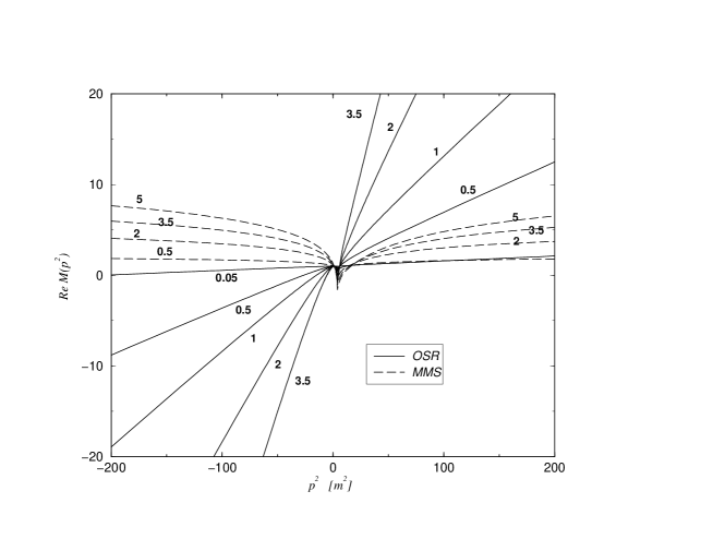
Figure 1: Dynamical mass of scalar particle in $\Phi^{3}$ theory calculated in bare vertex approximation in the both renormalization schemes. The lines are labeled by the value of $\lambda_{MMS}$ for MMS scheme and $\lambda_{OSR}$ for OSR renormalization scheme.

The critical value of $\lambda$ is simply defined by the collapse of ( numerically sophisticated) solution of the imaginary part DSEs. Before making a comparison of physical quantities we present the numerical results for the Green’s functions. In Fig.1 the so called dynamical mass

$$M(p^{2})=G^{-1}(p^{2})-p^{2}$$ (31)

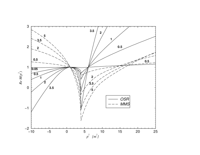
Figure 2: Infrared (threshold) details of the Fig.1.

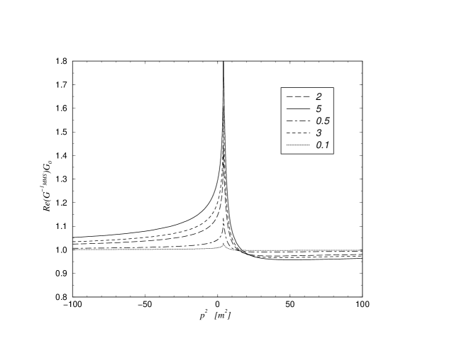
Figure 3: The propagators deviations from free theory. The propagator is calculated in minimal momentum renormalization scheme for various $\lambda_{MMS}$

of $\Phi^{3}$ theory boson is presented for various coupling strengths in both renormalization schemes. The infrared details are displayed in Fig.2. The dynamical mass is not directly physically observable since it is scheme dependent from the definition, the exception is the pole mass which is scheme independent and renormgroup invariant as well. It is interesting that there are time-like values of square of momenta where the propagators behave almost like free ones no matter how the coupling constant is strong. This happens somewhere around the point $p_{f}^{2}=6m^{2}$ for OSR scheme and approximately at $p_{f}^{2}=20m^{2}$ for MMS scheme, which implies the physical irrelevance of such a behavior (Of course, there are always differences within the absorptive parts $\pi\rho$ which are ordinarily coupling constant dependent at these points). The appropriate relevance of propagator dressing is best seen when the dressed propagator is compared with the free one $G=(p^{2}-m^{2})^{-1}$. From the Fig.3 and Fig.4. we can see that the propagator function is the most sensitive with respect to the self-energy correction for threshold momenta where these correction are enhanced about one magnitude, while they are largely suppressed for the above mentioned values of momenta $p_{f}^{2}$. Note that nothing from these things can be read from the purely Euclidean approach. The results presented up to now have been calculated in the bare vertex approximation, the solution with vertex correction included will be discussed bellow. The appropriate bar vertex approximation critical coupling value is $\lambda_{crit}^{OSR}\simeq 3.5$ for OSR scheme and $\lambda_{crit}^{MMS}\simeq 5$ for MMS scheme. Their different values are not a discrepancy but the necessary consequence of the renormalization scheme dependence.

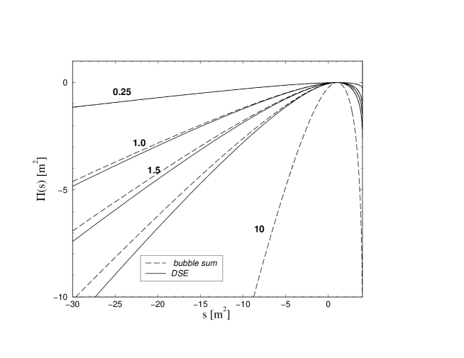
Figure 5: Comparison of DSE results in bare vertex approximation with the perturbation theory result. DSE and bubble summation is compared in OSR scheme. Each two close lines off different types correspond to the same value of coupling $\lambda_{OSR}=\{0.25;1.0;1.5;2.2\}$ . The lowest dashed line with $\lambda=10$ has not its DSE partner solution (since $\lambda>\lambda_{c}$).

Furthermore, in order to see the effect of self-consistency of DSE treatment we compare the DSE result with the perturbation theory in OSR scheme. From the Fig.5 we can see that the perturbation theory is perfectly suited method when applied somewhere bellow the critical value of the coupling. Therefore, the main goal of our solution is the information about the domain of validity of given model.

The issue of vertex improvement by the one loop skeleton diagram and its appropriate effect on the DSEs solution and scattering matrix is discussed in the text bellow. First let us note that the critical values of the couplings decrease and we have $\lambda_{crit}^{dressedvertex}\simeq\lambda_{crit}^{barevertex}/2$ which is roughly valid for both the renormalization scheme employed. We return to the question of meaning $\lambda_{crit}$ when we will discuss the WCM.

To make our comparison of proposed methods more meaningful, we do not compare the Green’s functions but rather wee look on the scattering amplitudes $M$ calculated in both renormalization schemes obtained in both truncations of DSEs. In Fig.6 we compare the imaginary parts of scattering amplitudes $M$ at a given kinematic channel. The comparison is made in the way proposed and described in the previous section. Henceforth, what are actually compared in this Figure are the Lehmann weights $\sigma$’s of the MMS scheme calculated for certain $\lambda_{MMS}$ and the rescaled Lehmann weights $r\sigma_{2}$ calculated for the OSR scheme with the appropriate coupling strength $\lambda_{OSR}=r\lambda_{MMS}$. It is apparent that the lines for $\Im mM_{OSR}(r\lambda_{MMS},t)$ and $\Im mM_{MMS}(\lambda_{MMS},t)$ for solutions with dressed vertices are much close each other then the solution with bare vertices. This statement is valid for all $t$ for a given theory characterized by its coupling constant (with $\lambda_{MMS}$ fixed). This is true for all couplings $\lambda^{\prime}s$, the only–but not so striking– exception is certain infrared excess for the value of couplings closed to the critical one. Of course, the worse numerical accuracy play the role in strong coupling. Nevertheless, we can see that when the approximation improves then there is apparent signal for achieving the renormalization scheme independence for all the values of the coupling constant.

In order to see aforementioned quantitative improvement we have calculated the appropriate deviations $E_{N},N=0,1$. The results for some larger value of the couplings are presented in the Tab.1. The corresponding difference becomes negligible when $\lambda$ decrease and approaches its ’perturbative’ value. For better orientation the infrared details for three choices of the coupling constants are also displayed in Fig.7.

3 DSEs for the WCM

The massive WCM is given by the following Lagrangian

$${\cal L}=\sum_{i}\frac{1}{2}\partial_{\mu}\Phi_{i}\partial^{\mu}\Phi_{i}-\sum_{i}\frac{1}{2}m_{i}^{2}\Phi_{i}^{2}+\left(\frac{g_{13}}{\sqrt{2}}\Phi_{1}^{2}+\frac{g_{23}}{\sqrt{2}}\Phi_{2}^{2}\right)\Phi_{3}+C.P.$$ (32)

where $C.P.$ means the appropriate counter-term part. Here we choose the second renormalization scheme employed in the previous section, i.e. the propagators of all three particles have the unit residua. All the definitions of counter-terms $\delta Z_{i},\delta m_{i},\delta g_{i}$ correspond with the OSR defined previously but now for each particle separately. Furthermore, we adjust the couplings to be

$$g_{i3}=\frac{Z_{g_{i3}}}{Z_{i}Z_{3}^{\frac{1}{2}}}g_{{i3}_{0}},\quad\quad i=1,2$$ (33)

such that

$$g_{13}=g_{23}.$$ (34)

The equal mass case $m_{1}=m_{2}$ was already solved [24] for purpose of studying the self-energy effect on the bound state spectrum. Here we solved the unequal mass case

$$\frac{m_{1}}{m_{2}}=4;\quad m_{3}=m_{2}$$ (35)

and compare the result with the Euclidean version of solution [16]. We restrict ourselves to the bare vertex approximation which is sufficient for comparison with [16]. Since all the derivation is rather straightforward we simply review the results. The renormalized DSEs in bare vertex approximation read

$$G_{Ri}^{-1}\left(p\right) = p^{2}-m_{i}^{2}-\Pi_{i(2)}(p^{2})\quad\quad i=1,2$$

$$G_{R3}^{-1}\left(p\right) = p^{2}-m_{3}^{2}-\Pi_{3(2)}(p^{2})$$

$$\Pi_{i}(p^{2}) = i2g^{2}\int\frac{d^{4}q}{\left(2\pi\right)^{4}}\,G_{3}\left(p-q\right)G_{i}\left(q\right)\quad\quad\quad i=1,2$$

$$\Pi_{3}(p^{2}) = ig^{2}\int\frac{d^{4}q}{\left(2\pi\right)^{4}}\,\sum_{i=1,2}G_{i}\left(p-q\right)G_{i}\left(q\right)$$ (36)

where the bracketed index denotes the renormalization scheme employed,and the second index labels the particle associated with the appropriate field in the Lagrangian (32). All the propagators satisfy the Lehmann representation with unit residuum and all the proper function obeys the double subtracted dispersion relation (2.2). Henceforth, the appropriate spectral weights are related through the relations

$$\sigma_{i}(\omega)=\frac{\rho_{i}(\omega)}{(\omega-m_{i}^{2})^{2}}+\frac{1}{(\omega-m_{i}^{2})}P.\int_{(m_{j}+m_{k})^{2}}^{\infty}d\alpha\frac{\sigma_{i}(\omega)\rho_{i}(\alpha)\left[\frac{\omega-m_{i}^{2}}{\alpha-m_{i}^{2}}\right]^{2}+\sigma_{i}(\alpha)\rho_{i}(\omega)}{\omega-\alpha},$$ (37)

where for the indices $i=1,2$ we have $j=2,3;k=3,3$ and for particle 3 the index $j=k=2$ since it label the lighter particle with the mass $m_{2}$. The expression for the absorptive parts read

$$\rho_{\pi_{i}}(\omega) = \frac{2g^{2}}{(4\pi)^{2}}\left[B(m_{i}^{2},m_{3}^{2};\omega)+\int_{0}^{\infty}d\alpha\left(B(\alpha,m_{i}^{2};\omega)\sigma_{3}(\alpha)+B(\alpha,m_{3}^{2};\omega)\sigma_{i}(\alpha)\right)\right.$$

$$+ \left.\int_{0}^{\infty}d\alpha d\beta B(\alpha,\beta;\omega)\sigma_{3}(\alpha)\sigma_{i}(\beta)\right],\quad\quad i=1,2$$

$$\rho_{\pi_{3}}(\omega) = \sum_{i=1,2}\frac{g^{2}}{(4\pi)^{2}}\left[\sqrt{1-\frac{4m_{i}^{2}}{\omega}}+2\int_{0}^{\infty}d\alpha B(\alpha,m_{i}^{2};\omega)\sigma_{i}(\alpha)\right.$$ (38)

$$+ \int_{0}^{\infty}\left.d\alpha d\beta B(\alpha,\beta;\omega)\sigma_{i}(\alpha)\sigma_{i}(\beta)\right].$$

where we freely integrate over the whole range of positive real axis leaving the information about the appropriate thresholds and subthresholds absorbed in the definition of the function $B$.

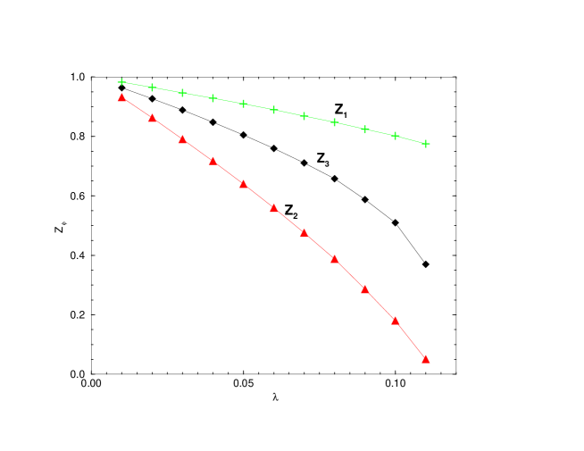
Figure 8: The dependence of field strength renormalization constants on the coupling strength of Wick-Cutkosky model. The index 1-3 labels the particle.

The above set of equations has been actually solved numerically. The main result for us is the appearance of the critical coupling strength $\lambda_{c}\equiv g_{c}^{2}/(4\pi m_{2}^{2})=0.12$ which rather accurately corresponds with the point where the renormalization constant $Z_{2}$ turns out to be negative. The appropriate dependence of the renormalization constants $Z_{i}$ is presented in Fig.8 for all three particle. The obtained critical value is in reasonable agreement with the one obtained by the Euclidean solution of DSEs system [16], where $\lambda_{c}=0.086$, as well as with the critical value $\lambda_{c}=0.063$ which was found using a variational approach [18],[19].

Furthermore, the existence of the critical coupling of OSR scheme can be seen from the analytical formula for the inverse of propagator

$$G_{i}^{-1}=p^{2}-m_{i}^{2}-\int_{0}^{\infty}d\alpha\frac{\rho_{i}(\alpha)(p^{2}-m_{i}^{2})^{2}}{(\alpha-m_{i}^{2})^{2}(p^{2}-\alpha+i\epsilon)}$$ (39)

which implies that for the strong enough coupling the Landau pole should appear, which must arise when the factor $L$

$$L=[1-\int_{0}^{\infty}\frac{\rho(\alpha)}{(\alpha-m^{2})^{2}}]$$ (40)

is negative (when it is just zero then the Landau pole is situated in space-like infinite, and for the positive $L$ this singularity never appears due to finiteness of the appropriate integral in (40)). For negative $L$ the propagator cannot satisfy Lehmann representation at all and at least the Minkowskian treatment used in this work must fail. Comparing equation (40) with the definition of renormalization constant $Z$ we clearly have the identification $L=Z$. As we have mentioned, the numerical solution start to fail when the condition $Z=0$ is fulfilled. This statement is justified with 10 % numerical accuracy. (We have no similar guidance for MMS scheme but we expect the similar appearance of the critical coupling $\lambda_{MMS}$ for this scheme as occured in $\Phi^{3}$ theory, but the reason for the numerical failure in this case is not found in this paper.)

4 Conclusion

We have obtained numerical solutions of the DSEs in Minkowski space for $\Phi^{3}$ theory and the WCM. This suggests that the expansion of the theory around the metastable vacuum leads to the predicative result. Our technique allows us to extract propagator spectral function $\rho(s)$ with reasonably high numerical accuracy. Since the renormalization procedure is performed analytically, it has no effect on the precision of solution. When the coupling does not exceed a certain critical value, then the domain of analyticity of the propagator is the all real axis of $p^{2}$. An attempt to clarified the meaning of critical coupling value was made. This suggests that it corresponds with appearance of unphysical singularity in the on-shell renormalized propagator. Consequently, the field renormalization constant (in on shell scheme) turns to be negative for $\lambda>\lambda_{crit}$.

Appendix A Dispersion relations for self-energies in bare vertex approximation

In this Appendix we derive DRs for self-energies in both renormalization schemes for the bare vertex. The calculation is very straightforward, and in fact it represents nothing else but evaluation of the one loop scalar Feynman diagram with different masses in internal lines.

Substituting the Lehmann representation for MMS propagators (2.2) the unrenormalized $\Pi$ can be split like

$$\Pi(p^{2}) = \Pi_{(b,b)}(p^{2})+2\Pi_{(b,s)}(p^{2})+\Pi_{(s,s)}(p^{2})$$

$$\Pi_{(b,b)}(p^{2}) = \int d\bar{q}\frac{18r^{2}g^{2}}{((p+q)^{2}-m^{2}+i\epsilon)(q^{2}-m^{2}+i\epsilon)}$$

$$\Pi_{(b,s)}(p^{2}) = \int d\bar{q}\int d\alpha\frac{18rg^{2}\sigma(\alpha)}{(q^{2}-\alpha+i\epsilon)((p+q)^{2}-m^{2}+i\epsilon)}$$

$$\Pi_{(s,s)}(p^{2}) = \int d\bar{q}\int d\alpha d\beta\frac{18g^{2}\sigma(\alpha)\sigma(\beta)}{((p+q)^{2}-\alpha+i\epsilon)(q^{2}-\beta+i\epsilon)},$$ (41)

where we have used shorthand notation for the measure $id^{4}q/(2\pi)^{4}\equiv d\bar{q}$. Making the subtraction, we immediately arrive for the pure perturbative contribution (up to the presence of the square of residuum):

$$\Pi_{1(b,b)} = \int_{4m^{2}}^{\infty}d\omega\frac{\rho_{1(b,b)}(p^{2}-m^{2})}{(p^{2}-\omega+i\epsilon)(\omega-m^{2})}$$

$$\rho_{1(b,b)}(\omega) = \frac{18r^{2}g^{2}}{(4\pi)^{2}}\sqrt{1-\frac{4m^{2}}{\omega}}$$ (42)

The most general integral to be solved is similar to the above case but with the physical masses replaced by the spectral variables.

$$I(p^{2})=\int d\bar{q}\frac{1}{((p+q)^{2}-\alpha)(q^{2}-\beta)}$$ (43)

which after the subtraction (44) and integration over the Feynman parameter $x$ leads to the appropriate single-subtracted DR (44)

$$I_{1s}(p^{2}) = I(p^{2})-I(m^{2})=\frac{1}{(4\pi)^{2}}\int_{0}^{[1]}dx\int_{\frac{m^{2}x+\alpha(1-x)}{x(1-x)}}^{\infty}d\omega\frac{(p^{2}-m^{2})}{(\omega-m^{2})(p^{2}-\omega+i\epsilon)}$$ (44)

$$= \int_{0}^{\infty}d\omega\frac{p^{2}-m^{2}}{(p^{2}-\omega+i\epsilon)}\frac{B(\alpha,\beta;\omega)}{(4\pi)^{2}(\omega-m^{2})},$$

where the function $B(u,v;\omega)$ is defined through the Khallen triangle function $\lambda$ like

$$B(u,v,\omega) = \frac{\lambda^{1/2}(u,\omega,v)}{\omega}\Theta\left(\omega-(\alpha^{\frac{1}{2}}+\beta^{\frac{1}{2}})^{2}\right)$$

$$\lambda(u,\omega,v) = (u-\omega-v)^{2}-4\omega v$$ (45)

$$= \omega^{2}+u^{2}+v^{2}-2\omega v-2\omega u-2uv.$$

It can be easy checked that $B(m^{2},m^{2};\omega)=\sqrt{1-\frac{4m^{2}}{\omega}}\Theta(\omega-4m^{2})$ which was already introduced in (A).

The OSR scheme requires additional subtraction which is finite and henceforth can proceed by making a simple algebra

$$I_{2s}(p^{2}) = I_{1s}(p^{2})-\frac{d}{dp^{2}}|_{p^{2}=m^{2}}I_{1s}(p^{2})$$ (46)

$$= \frac{1}{(4\pi)^{2}}\int_{0}^{\infty}d\omega\frac{(p^{2}-m^{2})^{2}}{(\omega-m^{2})^{2}(p^{2}-\omega+i\epsilon)}B(\alpha,\beta;\omega).$$

To summarize the results we see that MMS self-energy satisfies one subtracted DR with the absorptive part $\pi\rho_{1}$ given like

$$\rho_{\pi_{1}}(\omega) = \rho_{1(b,b)}(\omega)+2\rho_{1(b,s)}(\omega)+\rho_{1(s,s)}(\omega)$$

$$\rho_{1(b,b)}(\omega) = \frac{18r^{2}g^{2}}{(4\pi)^{2}}\sqrt{1-\frac{4m^{2}}{\omega}}$$

$$\rho_{1(b,s)}(\omega) = \int_{9m^{2}}^{\infty}d\alpha\frac{18rg^{2}}{(4\pi)^{2}}B(\alpha,m^{2};\omega)\sigma(\alpha)$$

$$\rho_{1(s,s)}(\omega) = \int_{16m^{2}}^{\infty}d\alpha d\beta\frac{18g^{2}}{(4\pi)^{2}}B(\alpha,\beta;\omega)\sigma(\alpha)\sigma(\beta)\quad,$$ (47)

while the self-energy in OSR scheme satisfies double subtracted DR with the absorptive part $\pi\rho_{2}$

$$\rho_{\pi_{2}}(\omega) = \rho_{2(b,b)}(\omega)+2\rho_{2(b,s)}(\omega)+\rho_{2(s,s)}(\omega)$$

$$\rho_{2(b,b)}(\omega) = \frac{18g^{2}}{(4\pi)^{2}}\sqrt{1-\frac{4m^{2}}{\omega}}$$

$$\rho_{2(b,s)}(\omega) = \int_{9m^{2}}^{\infty}d\alpha\frac{18g^{2}}{(4\pi)^{2}}B(\alpha,m^{2};\omega)\sigma_{2}(\alpha)$$

$$\rho_{2(s,s)}(\omega) = \int_{16m^{2}}^{\infty}d\alpha d\beta\frac{18g^{2}}{(4\pi)^{2}}B(\alpha,\beta;\omega)\sigma_{2}(\alpha)\sigma_{2}(\beta).$$ (48)

Appendix B Two-loop skeleton self-energy DR

The finite two-loop integral appears after the substitution of the vertex (11) to the self-energy formula

$$\int d\bar{q}d\bar{k} \left[(k^{2}-\alpha_{1}+i\epsilon)((p+k)^{2}-\alpha_{2}+i\epsilon)((k-q)^{2}-\alpha_{3}+i\epsilon)\right.$$ (49)

$$\left.(q^{2}-\alpha_{4}+i\epsilon)((p+q)^{2}-\alpha_{5}+i\epsilon)\right]^{-1}$$

where all the irrelevant pre-factors are omitted for purpose of the brevity. They will be correctly added at the end of calculation for both renormalization schemes separately. The contribution is ultraviolet finite therefore we first calculate the unrenormalized result. Firstly, we parameterize the off-shell vertex by matching the first three denominators and consequently we integrate over the triangle loop momentum $k$

$$\int\bar{k}\left[(k^{2}-\alpha_{1}+i\epsilon)((p+k)^{2}-\alpha_{2}+i\epsilon)((k-q)^{2}-\alpha_{3}+i\epsilon)\right]^{-1}=$$

$$\int\bar{k}\int_{0}^{1}dxdy2y\left[k^{2}xy+(p+k)^{2}(1-x)y+(k-q)^{2}(1-y)\right.$$

$$-\left.\alpha_{1}xy-\alpha_{2}(1-x)y-\alpha_{3}(1-y)+i\epsilon\right]^{-3}=$$ (50)

$$\int_{0}^{1}\frac{dxdyy}{(4\pi)^{2}}\left[p^{2}(1-x)y(1-(1-x)y)+q^{2}y(1-y)+2p.q(1-x)y(1-y)\right.$$

$$\left.-\alpha_{1}xy-\alpha_{2}(1-x)y-\alpha_{3}(1-y)+i\epsilon\right]^{-1}.$$

Next, we substitute $x\rightarrow 1-x$ and after some algebra we obtain for equation (B)

$$\int_{0}^{1}\frac{dxdy}{(4\pi)^{2}(1-y)}\left[q^{2}+2p.qx+p^{2}\frac{x(1-xy)}{(1-y)}-O_{1-3}+i\epsilon\right]^{-1}$$ (51)

where we have used short notation $O_{1-3}=\alpha_{1}\frac{1-x}{1-y}+\alpha_{2}\frac{x}{1-y}+\alpha_{3}\frac{1}{y}$. We continue by matching equation (51) with two spare denominators in (49) by using Feynman variables $z$ and $u$ for denominators with $\alpha_{4}$ and $\alpha_{5}$, respectively. Then we can write for (49)

$$\int d\bar{q}\int_{0}^{1}\frac{dxdydzdu2u}{4\pi)^{2}(1-y)}\left[q^{2}+2p.qxzu+2p.q(1-u)\right.$$

$$+\left.p^{2}\frac{(1-xy)xzu}{(1-y)}+p^{2}(1-u)-O_{1-5}+i\epsilon\right]^{-3}$$ (52)

where we have used shorthand notation $O_{1-5}=O_{1-3}zu+\alpha_{4}(1-z)u+\alpha_{5}(1-u)$. Shifting $q+p(xzu+1-u)\rightarrow q$ and integrating over new $q$ it yields:

$$\int_{0}^{1}\frac{dxdydzduu}{(4\pi)^{4}(1-y)F(x,y,z)}\frac{1}{\left[p^{2}-\frac{O_{1-5}}{F(x,y,z)}+i\epsilon\right]}$$

$$F(x,y,z)=1-u+\frac{(1-xy)xzu}{(1-y)}-(xzu+(1-u))^{2}$$ (53)

Next we substitute $u\rightarrow\omega$ where $\omega=O_{1-5}/F(x,y,z)$. Using the notation

$$\omega = \frac{ua_{1}+a_{2}}{u^{2}b_{1}+ub_{2}}$$ (54)

$$a_{1} = (\alpha_{1}(1-x)y+\alpha_{2}xy+\alpha_{3}(1-y))z+(\alpha_{4}(1-z)-\alpha_{5})y(1-y)$$

$$a_{2} = \alpha_{5}y(1-y)$$

$$b_{1} = -(1-xz)^{2}y(1-y)$$

$$b_{2} = (1-2xz)y(1-y)+(1-xy)xyz\quad,$$ (55)

we can write down the appropriate DR for equation (49)

$$\Omega(\omega;\alpha_{1},..\alpha_{5}) = \int_{0}^{\infty}\frac{d\omega}{p^{2}-\omega+i\epsilon}\int_{0}^{1}\frac{dxdydz}{(4\pi)^{4}(1-y)}\frac{\Theta\left(\omega-\frac{a_{1}+a_{2}}{b_{1}+b_{2}}\right)\Theta(D)}{\left[\frac{\alpha_{5}}{U^{2}}-\omega(1-xz)^{2}\right]}$$ (56)

$$U = \frac{-B+\sqrt{D}}{2A};\quad D=B^{2}-4AC$$

$$A = \omega b_{1};\quad B=\omega b_{2}-a_{1};\quad C=-a_{2}\quad.$$

Note here that spectral function (everything after the first fraction in (56) is always positive for allowed values of $\alpha^{\prime}s$ and it is regular function of its argument $\omega$. The various subthresholds are then given by the values of Lehmann variables $\alpha$’s in accordance with the step function presented, noting that the perturbative threshold is given again by $4m^{2}$ and in that case case the result partially simplified. For completeness we reviewed the associated simplifications, namely: $a_{1}=m^{2}z(1-y(1-y));\quad a_{2}=m^{2}y(1-y)$. Making one subtraction for the MMS and two subtraction for OSR scheme we can recognize that the appropriate skeleton DR for master diagram has the absorptive part

$$\rho_{1}^{[2]}(\omega)=\frac{(6g)^{4}}{2}\prod_{i=1}^{5}\int d\alpha_{i}\tilde{\sigma}(\alpha_{i})\Omega(\omega,\alpha_{1},..\alpha_{2})$$ (57)

for MMS scheme and

$$\rho_{2}^{[2]}(\omega)=\frac{(6g_{2})^{4}}{2}\prod_{i=1}^{5}\int d\alpha_{i}\tilde{\sigma}_{2}(\alpha_{i})\Omega(\omega,\alpha_{1},..\alpha_{2})$$ (58)

for OSR scheme, respectively. In fact it gives rise 28 various contributions to $\rho^{[2]}$ (only 12 are actually topologically independent, distinguished by the number of continuous Lehmann weights with the appropriate position of spectral variable in $\Omega$.) All of them have been found numerically for the purpose of DSEs solution.

TABLE 1. Normalized and weighted integral deviations $E_{N}$ between scattering amplitudes calculated in the OSR and MMS scheme. Exact scheme independence corresponds to the case $E_{N}=0$. The parameters $N=1$ makes the quantity $E$ more sensitive to the systematic error in the infrared domain. The denotation BV(DV) means that the appropriate propagator was calculated with bare (dressed) vertex. The function $E$ is displayed for three cases of results presented in Figures 6 and 7.

Figure 4: The propagator deviation from free theory. The propagator is calculated in on mass-shell renormalization scheme with unit residuum for various $\lambda_{OSR}$.

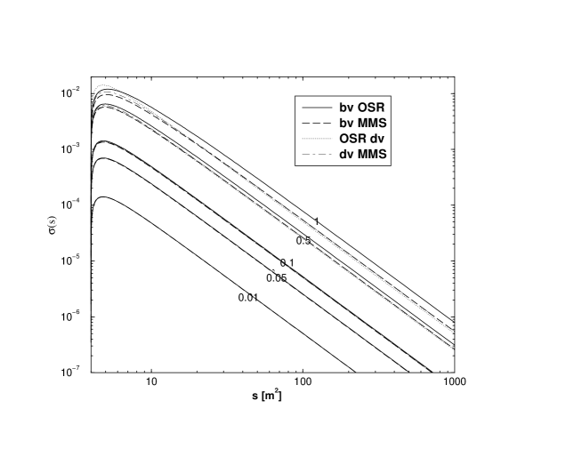
Figure 6: Imaginary parts of scattering matrix calculated with propagator which have been obtained in MMS and OSR scheme with (dv) and without (bv) improved vertex. Each set of lines corresponding to the same model is labeled by the coupling strength $\lambda_{MMS}$.

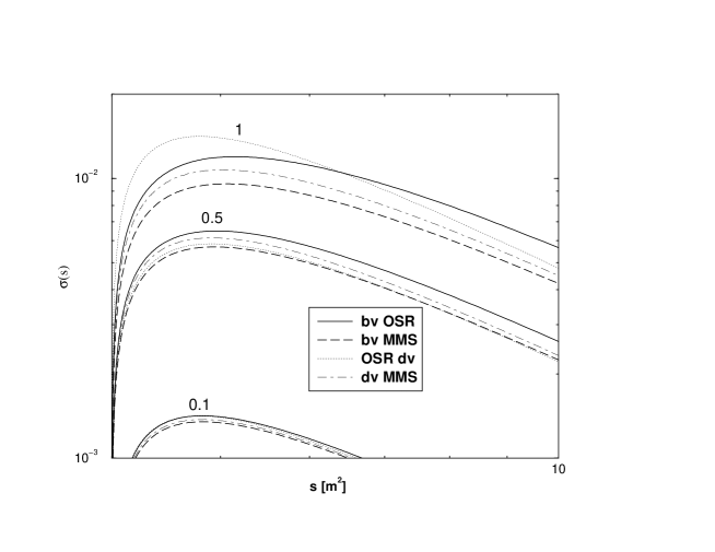
Figure 7: The low frequency details of the Fig.6.

References

- [1] A. Salam, Phys. Rev. 130, 1287 (1963).
- [2] R. Delbourgo, Nuovo Cimento 49, 484 (1979).
- [3] R. Delbourgo and G. Thompson J. Phys. G8, L185 (1982).
- [4] R. Delbourgo and R.B. Zhang, J. Phys. 17A, 3593 (1984).
- [5] J.M.Cornwal, R. Jackiw and E.T. Tomboulis, Phys. Rev. D 10, 2428 (1974).
- [6] Silvan S. Schweber, An Introduction to Relativistic Quantum Field Theory , Row, Peterson and Co*Evanston, Ill., Elmsford, N.Y.,(1969).
- [7] C.D. Roberts and A.G. Williams, Prog. Part. Nucl. Phys. 33, 477 (1994).
- [8] J.C. Collins, Renormalization Cambridge University Press, 1984.
- [9] W. Celmaster and D. Sivers, Phys. Rev. D 23, 227 (1981).
- [10] V.Šauli, JHEP 0302 (2003) 001, (hep-ph/0209046).
- [11] G.Baym, Phys. Rev. 117, 886 (1960).
- [12] J.M.Cornwal, Phys.Rev. D55, 6209 (1997).
- [13] J.M.Cornwal, Phys.Rev. D52,6074 (1995).
- [14] R. Delbourgo, D. Elliott, D. McAnally, Phys. Rev. D 55, 5230 (1997).
- [15] D.J. Broadhurst, D.Kreimer, Nucl.Phys. B 600,403 (2001).
- [16] S. Ahlig, R. Alkofer, Annals Phys. 275, 113 (1999).
- [17] T. Nieuwenhuis and J.A. Tjon, Few Body Syst. 21,167 (1996).
- [18] R. Rosenfelder and A.W. Schreiber, Phys.Rev. D 53, 3337 (1996).
- [19] R. Rosenfelder and A.W. Schreiber, Phys.Rev. D 53, 3354 (1996).
- [20] J. Polchinski, Nucl. Phys. B231, 269 (1984).
- [21] T.R. Morris, Int. J. Mod. Phys A9, 2411 (1994).
- [22] C. Itzykson and J.B. Zuber, Quantum Field Theory, McGraw-Hill Inc. (1980).
- [23] W. Detmold, Phys.Rev. D 67,085011 (2003).
- [24] V.Šauli and J.Adam, Phys.Rev. D 67,044304 (2003).
- [25] G.t’ Hooft and M.J.G. Veltman, Nucl. Phys. B44, 189 (1972).
- [26] G. Grunberg, Phys. Rev. D 29, 2315 (1984).
- [27] J. Fischer, Int.J.Mod.Phys. A12, 3625 (1997).
- [28] A.W. Schreiber, T. Sizer and A.G. Williams Phys.Rev. D 58, 125014 (1998).