SLAC-PUB-9585 November 2002

Constraining the Littlest Higgs

JoAnne L. Hewett, Frank J. Petriello, and Thomas G. Rizzo Stanford Linear Accelerator Center

Stanford University

Stanford CA 94309, USA

Little Higgs models offer a new way to address the hierarchy problem, and give rise to a weakly-coupled Higgs sector. These theories predict the existence of new states which are necessary to cancel the quadratic divergences of the Standard Model. The simplest version of these models, the Littlest Higgs, is based on an $SU(5)/SO(5)$ non-linear sigma model and predicts that four new gauge bosons, a weak isosinglet quark, $t^{\prime}$, with $Q=2/3$, as well as an isotriplet scalar field exist at the TeV scale. We consider the contributions of these new states to precision electroweak observables, and examine their production at the Tevatron. We thoroughly explore the parameter space of this model and find that small regions are allowed by the precision data where the model parameters take on their natural values. These regions are, however, excluded by the Tevatron data. Combined, the direct and indirect effects of these new states constrain the ‘decay constant’ $f\mathrel{\mathchoice{\lower 3.01385pt\vbox{\halign{$\matth\displaystyle\hfil#\hfil$\cr>\crcr\sim\crcr}}}{\lower 3.01385pt\vbox{\halign{$\matth\textstyle\hfil#\hfil$\cr>\crcr\sim\crcr}}}{\lower 3.01385pt\vbox{\halign{$\matth\scriptstyle\hfil#\hfil$\cr>\crcr\sim\crcr}}}{\lower 3.01385pt\vbox{\halign{$\matth\scriptscriptstyle\hfil#\hfil$\cr>\crcr\sim\crcr}}}}3.5$ TeV and $m_{t^{\prime}}\mathrel{\mathchoice{\lower 3.01385pt\vbox{\halign{$\matth\displaystyle\hfil#\hfil$\cr>\crcr\sim\crcr}}}{\lower 3.01385pt\vbox{\halign{$\matth\textstyle\hfil#\hfil$\cr>\crcr\sim\crcr}}}{\lower 3.01385pt\vbox{\halign{$\matth\scriptstyle\hfil#\hfil$\cr>\crcr\sim\crcr}}}{\lower 3.01385pt\vbox{\halign{$\matth\scriptscriptstyle\hfil#\hfil$\cr>\crcr\sim\crcr}}}}7$ TeV. These bounds imply that significant fine-tuning be present in order for this model to resolve the hierarchy problem.

1 Introduction

The Standard Model (SM) of electroweak physics is a remarkable achievement. Precision electroweak experiments have probed the SM at the level of quantum effects and have confirmed every feature of the theory. In particular, the set of precision electroweak (EW) data has tested the SM beyond one-loop level and no significant deviations from SM predictions have been observed. The symmetry breaking sector of the SM has been investigated through its virtual effects and precision measurements strongly prefer the existence of a weakly coupled Higgs boson by constraining its mass to be $m_{H}<193$ GeV at $95\%$ CL [1]. This upper bound may be relaxed if certain classes of new physics contributions beyond the SM are present at the TeV scale and compensate for the indirect effects of a heavier scalar sector [2]. However, because of decoupling, models with an elementary Higgs scalar typically yield small contributions to the electroweak radiative corrections. Direct evidence for the electroweak symmetry breaking dynamics has yet to be observed, and searches for Higgs boson production have placed the compatible lower bound $m_{H}>114.4$ GeV.

The existence of a weakly coupled Higgs sector generates the hierarchy problem, which is a long-standing puzzle in particle physics. Few candidates exist for the mechanism which solves this problem. Supersymmetry naturally stabilizes the hierarchy, as the quadratically divergent loop contributions to the Higgs mass cancel between the fermion and boson contributions, provided the supersymmetry breaking scale is near a TeV [3]. Novel theories with extra dimensions exploit the geometry of the higher dimensional spacetime to resolve the hierarchy [4] and result in numerous phenomenological consequences at the TeV scale [5]. Supersymmetry has the additional feature of remaining weakly coupled up to high scales, whereas quantum gravity becomes strong at the TeV scale in these extra-dimensional models. Experimental confirmation of either scenario has yet to occur.

Recently, another scenario has been developed which attacks the hierarchy problem in a new way, while maintaining a weakly coupled scalar sector. This scenario is known as the Little Higgs [6, 7] where the Higgs is effectively a pseudo-Goldstone boson. These theories are realizations of earlier attempts [8] to stablize a Higgs which arises as a pseudo-Goldstone boson resulting from a spontaneously broken non-linear approximate symmetry. This approximate global symmetry protects the Higgs vev relative to the UV cut-off of the theory, $\Lambda$, which appears at a higher scale. The recent progress was attained in models of dimensional deconstruction [9], where the quadratically divergent corrections to the Higgs mass were shown to cancel with contributions from new fields in non-trivial descriptions of theory space. The phenomenology of these models was examined in [10]. The recent Little Higgs models have the advantage of not requiring a non-trivial theory space in order for the quadratic divergences to be eliminated. The novel feature of these cancellations, is that the divergent contributions from a particular particle are cancelled by a new particle of the same spin. Hence, these theories predict the existence of new $Q=+2/3$ quarks, gauge bosons, and scalars, all with masses at the TeV scale, in order to remove the relevant divergences. In addition, a small mass for the Higgs boson, of order 100 GeV, is naturally obtained from multi-loop corrections.

The most economical model of this type to date, known as the Littlest Higgs [6], is based on an $SU(5)/SO(5)$ nonlinear sigma model. The UV cut-off of this theory occurs at $\Lambda\sim 4\pi f\sim 10$ TeV, where the nonlinear sigma model becomes strongly coupled. Here $f$ is the decay constant of the pseudo-Goldstone boson and is necessarily of order a TeV. The $SU(5)\rightarrow SO(5)$ symmetry breaking is generated at the scale $\Lambda$ by strong interactions similar to technicolor which act only at the high scale $\Lambda$ and have no remnants at a TeV. The 14 Goldstone bosons remaining after this symmetry breaking yield a physical doublet and a complex triplet under $SU(2)$; the remaining fields are eaten by a Higgs-like mechanism when the intermediate symmetry is broken. The one-loop contributions to the quadratic divergences from the electroweak gauge sector are removed by making use of the $SU(5)$ weakly gauged subgroup $[SU(2)\times U(1)]^{2}$. The divergent contributions must then involve couplings of both groups and hence first appear at two-loop order. This combination of gauge couplings breaks the global symmetries and generates a small mass of order 100 GeV at the two-loop level for the scalar doublet field. At one-loop order, the Higgs mass is not sensitive to the effective high scale $\Lambda$, and its mass is thus relatively stable assuming $\Lambda\sim 10$ TeV. The scalar triplet acquires a mass at the TeV scale from one-loop gauge interactions. A massive vector-like $SU(2)$ singlet $Q=+2/3$ quark is responsible for canceling the one-loop divergences originating from the SM top-quark.

The physical spectrum of this model below a TeV is thus simply that of the SM with a single light Higgs. At the TeV scale four new gauge bosons $V_{i}$ (an electroweak triplet and singlet) appear, as well as the scalar triplet $\phi$, and a single vector-like quark $t^{{}^{\prime}}$. For the quadratically divergent corrections to cancel naturally, and not be fine-tuned, the mass of the new quark is constrained to be [6]

$$m_{t^{\prime}}\mathrel{\mathchoice{\lower 3.01385pt\vbox{\halign{$\matth\displaystyle\hfil#\hfil$\cr<\crcr\sim\crcr}}}{\lower 3.01385pt\vbox{\halign{$\matth\textstyle\hfil#\hfil$\cr<\crcr\sim\crcr}}}{\lower 3.01385pt\vbox{\halign{$\matth\scriptstyle\hfil#\hfil$\cr<\crcr\sim\crcr}}}{\lower 3.01385pt\vbox{\halign{$\matth\scriptscriptstyle\hfil#\hfil$\cr<\crcr\sim\crcr}}}}2~{}{\rm TeV}\left[{m_{H}\over 200~{}{\rm GeV}}\right]^{2}\,,$$ (1)

which in turn implies

$$f\mathrel{\mathchoice{\lower 3.01385pt\vbox{\halign{$\matth\displaystyle\hfil#\hfil$\cr<\crcr\sim\crcr}}}{\lower 3.01385pt\vbox{\halign{$\matth\textstyle\hfil#\hfil$\cr<\crcr\sim\crcr}}}{\lower 3.01385pt\vbox{\halign{$\matth\scriptstyle\hfil#\hfil$\cr<\crcr\sim\crcr}}}{\lower 3.01385pt\vbox{\halign{$\matth\scriptscriptstyle\hfil#\hfil$\cr<\crcr\sim\crcr}}}}1~{}{\rm TeV}\left[{m_{H}\over 200~{}{\rm GeV}}\right]^{2}\,.$$ (2)

In addition, naturalness also implies

$$m_{V_{i}}\mathrel{\mathchoice{\lower 3.01385pt\vbox{\halign{$\matth\displaystyle\hfil#\hfil$\cr<\crcr\sim\crcr}}}{\lower 3.01385pt\vbox{\halign{$\matth\textstyle\hfil#\hfil$\cr<\crcr\sim\crcr}}}{\lower 3.01385pt\vbox{\halign{$\matth\scriptstyle\hfil#\hfil$\cr<\crcr\sim\crcr}}}{\lower 3.01385pt\vbox{\halign{$\matth\scriptscriptstyle\hfil#\hfil$\cr<\crcr\sim\crcr}}}}6~{}{\rm TeV}\left[{m_{H}\over 200~{}{\rm GeV}}\right]^{2}\,,\quad\quad\quad m_{\phi}\mathrel{\mathchoice{\lower 3.01385pt\vbox{\halign{$\matth\displaystyle\hfil#\hfil$\cr<\crcr\sim\crcr}}}{\lower 3.01385pt\vbox{\halign{$\matth\textstyle\hfil#\hfil$\cr<\crcr\sim\crcr}}}{\lower 3.01385pt\vbox{\halign{$\matth\scriptstyle\hfil#\hfil$\cr<\crcr\sim\crcr}}}{\lower 3.01385pt\vbox{\halign{$\matth\scriptscriptstyle\hfil#\hfil$\cr<\crcr\sim\crcr}}}}10~{}{\rm TeV}\,.$$ (3)

The Littlest Higgs, based on a $SU(5)/SO(5)$ non-linear sigma model, is the simplest scenario of this type in the sense that it introduces a minimal number of new fields. Other models have been investigated [7] and are based on the cosets $SU(k)/Sp(k)$, $SU(k)^{2}/SU(k)$, and $SU(k)^{n}/SU(k)^{m}$, where $k$ is the number of strongly interacting fermions at the scale $\Lambda$. These cases differ from the Littlest Higgs in that they require the introduction of additional scalars, gauge bosons, and vector-like quarks at the TeV scale, and sometimes extra light scalar fields can arise at $\sim 100$ GeV.

In this paper, we examine the effects of the components of the Little Higgs on precision electroweak observables and in direct searches for new particles. We concentrate on the minimal model here, the Littlest Higgs [6], as it contains all the essential ingredients and provides a representative example of these types of theories. We would expect the more complicated scenarios listed above to be even further constrained by experiment in the absence of any fine-tuning due to the presence of the additional new particles at the TeV scale. Consistency with the global precision electroweak data set is a tough barrier for any new model to pass, and we find that the Littlest Higgs does not necessarily decouple quickly enough for most of the parameter space. A thorough examination of the parameter space reveals small regions where precision data, alone, allows for scales in the theory to take on their natural values, i.e., $f\mathrel{\mathchoice{\lower 3.01385pt\vbox{\halign{$\matth\displaystyle\hfil#\hfil$\cr<\crcr\sim\crcr}}}{\lower 3.01385pt\vbox{\halign{$\matth\textstyle\hfil#\hfil$\cr<\crcr\sim\crcr}}}{\lower 3.01385pt\vbox{\halign{$\matth\scriptstyle\hfil#\hfil$\cr<\crcr\sim\crcr}}}{\lower 3.01385pt\vbox{\halign{$\matth\scriptscriptstyle\hfil#\hfil$\cr<\crcr\sim\crcr}}}}2$ TeV. However, we find that the most stringent constraint arises from the direct search for new gauge bosons in Drell-Yan production at the Tevatron [11] and that this excludes these regions. Together, the direct and indirect data samples place the constraints $f\mathrel{\mathchoice{\lower 3.01385pt\vbox{\halign{$\matth\displaystyle\hfil#\hfil$\cr>\crcr\sim\crcr}}}{\lower 3.01385pt\vbox{\halign{$\matth\textstyle\hfil#\hfil$\cr>\crcr\sim\crcr}}}{\lower 3.01385pt\vbox{\halign{$\matth\scriptstyle\hfil#\hfil$\cr>\crcr\sim\crcr}}}{\lower 3.01385pt\vbox{\halign{$\matth\scriptscriptstyle\hfil#\hfil$\cr>\crcr\sim\crcr}}}}3.5-4.0$ TeV, and $m_{t^{\prime}}\mathrel{\mathchoice{\lower 3.01385pt\vbox{\halign{$\matth\displaystyle\hfil#\hfil$\cr>\crcr\sim\crcr}}}{\lower 3.01385pt\vbox{\halign{$\matth\textstyle\hfil#\hfil$\cr>\crcr\sim\crcr}}}{\lower 3.01385pt\vbox{\halign{$\matth\scriptstyle\hfil#\hfil$\cr>\crcr\sim\crcr}}}{\lower 3.01385pt\vbox{\halign{$\matth\scriptscriptstyle\hfil#\hfil$\cr>\crcr\sim\crcr}}}}7$ TeV, indicating that significant fine-tuning is required if this scenario is to work.

The outline for the remainder of this paper is as follows: in the next section we present the formalism for our analysis. We start with a description of the parameters in this theory and then give a derivation of the shifts that occur in the precision electroweak observables. In section 3, we present our numerical results. We first examine the bounds obtained from direct searches for new gauge bosons at the Tevatron. We then study the case where the new particles take on SM values for their coupling strengths and perform a fit to the electroweak data set and obtain tight constraints on the model. We then vary these couplings within natural ranges and demonstrate that there is a region of parameter space where the precision data bounds are relaxed, but is still excluded by the Tevatron data. The final section contains our conclusions.

2 Formalism

To begin our analysis, we follow the notation of Arkani-Hamed et al.[6] and generate the masses of the $[SU(2)\times U(1)]^{2}$ gauge bosons through the leading two-derivative kinetic term for the non-linear sigma model

$${\cal L}={f^{2}\over{4}}Tr|D_{\mu}\Sigma|^{2}\,,$$ (4)

where $f\sim 1$ TeV and the $\Sigma=exp(2i\Pi/f)\Sigma_{0}$ represents the Goldstone boson fields. The fourteen fields $\Pi$ include the SM weak iso-doublet $h$, an isotriplet $\phi$ as well as the true Goldstone bosons which are eaten in the breaking of the intermediate symmetry to the SM. We choose the normalization

$$\Pi=\left(\begin{array}[]{ccc}&h^{\dagger}/2&\phi^{\dagger}/\sqrt{2}\\ h/2&&h^{*}/2\\ \phi/\sqrt{2}&h^{T}/2&\end{array}\right)$$ (5)

such that the normalization of the kinetic term above is in agreement with that in earlier work on the non-linear sigma model [12]. In addition to the usual Higgs doublet vev, the triplet $\phi$ also acquires an $SU(2)$ breaking vev. We demonstrate in the Appendix that including the contribution from the triplet vev to the precision electroweak observables only strengthens our conclusions; here we adopt a conservative approach and neglect this piece in the following. We note that the presence of a scalar triplet is not a generic feature of Little Higgs models. The covariant derivative of $\Sigma$ is given by

$$D\Sigma=\partial\Sigma-ig_{k}W^{a}_{k}(Q^{a}_{k}\Sigma+\Sigma Q^{aT}_{k})-ig_{k}^{\prime}B_{k}(Y_{k}\Sigma+\Sigma Y^{T}_{k})\,,$$ (6)

where a sum over the index $k=1,2$ is understood and the ‘charge’ ($Q^{a}$) and ‘hypercharge’ ($Y$) matrices are given in Ref. [6]. To proceed further in the calculation of the gauge boson masses it is useful to define the following combinations of the above $[SU(2)\times U(1)]_{k}$ gauge couplings:

$$g = \frac{g_{1}g_{2}}{\sqrt{g_{1}^{2}+g_{2}^{2}}}\,\,,\;\;\;g^{{}^{\prime}}=\frac{g^{{}^{\prime}}_{1}g^{{}^{\prime}}_{2}}{\sqrt{g^{{}^{\prime}2}_{1}+g^{{}^{\prime}2}_{2}}}\,\,,$$

$$g_{t} = \frac{g^{2}_{1}}{\sqrt{g_{1}^{2}+g_{2}^{2}}}\,\,,\;\;\;g^{{}^{\prime}}_{t}=\frac{g^{{}^{\prime}2}_{1}}{\sqrt{g^{{}^{\prime}2}_{1}+g^{{}^{\prime}2}_{2}}}\,\,.$$ (7)

Inverting these relations yields

$$g_{1} = (g^{2}+g_{t}^{2})^{1/2}\,,$$

$$g_{2} = {g\over{g_{t}}}(g^{2}+g_{t}^{2})^{1/2}\,,$$ (8)

and similarly for $g_{1,2}^{\prime}$. To zeroth-order in the Higgs vev, one linear combination of the gauge bosons obtains a mass at the TeV scale when the intermediate symmetry is broken, while the second set remains massless. The massive neutral fields and their corresponding masses are given by

$$B_{h} = \frac{g^{{}^{\prime}}_{1}B_{1}-g^{{}^{\prime}}_{2}B_{2}}{\sqrt{g^{{}^{\prime}2}_{1}+g^{{}^{\prime}2}_{2}}}\,\,,\;\;\;m_{B_{h}}^{2}=\frac{1}{10}\frac{\left(g^{{}^{\prime}2}+g^{{}^{\prime}2}_{t}\right)^{2}}{g^{{}^{\prime}2}_{t}}f^{2}\,\,,$$

$$Z_{h} = \frac{g_{1}W^{3}_{1}-g_{2}W^{3}_{2}}{\sqrt{g^{2}_{1}+g^{2}_{2}}}\,\,,\;\;\;m_{Z_{h}}^{2}=\frac{1}{2}\frac{\left(g^{2}+g^{2}_{t}\right)^{2}}{g^{2}_{t}}f^{2}\,\,.$$ (9)

The corresponding charged isospin partner of the $Z_{h}$, $W_{h}^{\pm}$, obtains an identical mass:

$$W^{\pm}_{h}=\frac{g_{1}W^{\pm}_{1}-g_{2}W^{\pm}_{2}}{\sqrt{g_{1}^{2}+g_{2}^{2}}}\,\,,\;\;\;m_{W_{h}}^{2}=\frac{1}{2}\frac{\left(g^{2}+g^{2}_{t}\right)^{2}}{g^{2}_{t}}f^{2}\,\,.$$ (10)

The orthogonal linear combinations

$$B^{(0)} = \frac{g^{{}^{\prime}}_{2}B_{1}+g^{{}^{\prime}}_{1}B_{2}}{\sqrt{g^{{}^{\prime}2}_{1}+g^{{}^{\prime}2}_{2}}}\,\,,$$

$$W^{3(0)} = \frac{g_{2}W^{3}_{1}+g_{1}W^{3}_{2}}{\sqrt{g^{2}_{1}+g^{2}_{2}}}\,\,,$$ (11)

together with the corresponding charged field, $W^{\pm(0)}$, remain massless at this order. They will play the roles of the SM fields and acquire masses through the usual Higgs mechanism which are proportional to the Higgs vev, $\nu$.

In performing the comparison to precision electroweak and collider data, one must include the shifts in the SM-like gauge boson masses due to mixing with the heavier states, i.e., the Higgs vev induces a finite mixing between the states $B_{h},Z_{h},W_{h}$ and the corresponding lighter fields. For the neutral fields, which form a $4\times 4$ mass matrix, this mixing is most easily examined via a power series expansion in the ratio of the Higgs vev relative to $f$. For the charged fields, since the mass matrices are now only $2\times 2$, exact eigenvalues in a compact form can be easily found. The leading corrections to the masses of the lighter SM-like fields are of relative order $\delta^{2}=(\nu/f)^{2}\sim 0.01$ so that, numerically, $\delta^{4}$ corrections can be safely neglected. When discussing the effects of the heavy gauge fields on precision measurements, we will consistently keep all terms of relative order $\delta^{2}$. Turning now to the light mass eigenstates, we define the zeroth-order weak mixing angle as follows:

$$c_{W}^{(0)}=\frac{g}{\sqrt{g^{2}+g^{{}^{\prime}2}}}\,,\;\;\;\;s_{W}^{(0)}=\frac{g^{{}^{\prime}}}{\sqrt{g^{2}+g^{{}^{\prime}2}}}\,,$$ (12)

so that the physical $\gamma$ and $Z$ bosons become (to ${\cal O}\left(\delta^{2}\right)$)

$$A = c_{W}^{(0)}B^{(0)}-s_{W}^{(0)}W^{3(0)}\,\,,$$

$$Z = c_{W}^{(0)}W^{3(0)}+s_{W}^{(0)}B^{(0)}+\delta_{B_{h}}B_{h}+\delta_{Z_{h}}Z_{h}\,\,,$$ (13)

where $\delta_{B_{h}}\,,\delta_{Z_{h}}$ are defined below in Eq. 15. For the physical $W^{\pm}$ bosons we obtain

$$W^{\pm}=\frac{g_{2}}{\sqrt{g_{1}^{2}+g_{2}^{2}}}\left\{1-\frac{g_{1}^{2}\left(g_{1}^{2}-g_{2}^{2}\right)}{4\left(g_{1}^{2}+g_{2}^{2}\right)^{2}}\delta^{2}\right\}W^{\pm}_{1}+\frac{g_{1}}{\sqrt{g_{1}^{2}+g_{2}^{2}}}\left\{1+\frac{g_{2}^{2}\left(g_{1}^{2}-g_{2}^{2}\right)}{4\left(g_{1}^{2}+g_{2}^{2}\right)^{2}}\delta^{2}\right\}W^{\pm}_{2}\,\,,$$ (14)

which can easily be written in terms of the unmixed fields $W^{\pm(0)}$ and $W_{h}^{\pm}$,

$$W^{\pm}=W^{\pm(0)}-{g_{1}g_{2}(g_{1}^{2}-g_{2}^{2})\over{4(g_{1}^{2}+g_{2}^{2})^{2}}}\delta^{2}~{}W_{h}^{\pm}\,.$$ (15)

Note that the mixing between these states vanishes in the limit $g_{1}=g_{2}$ or, more specifically, when $g_{t}=g$. The physical $Z$ contains a small admixture of the heavy fields proportional to $\delta_{B_{h}},\delta_{Z_{h}}$. These parameters, which define the mixing between the light SM-like $Z$ and the heavy neutral gauge bosons, are given to order $\delta^{2}$ by:

$$\delta_{B_{h}} = -\frac{5}{4}\frac{g^{{}^{\prime}}_{t}\left(g^{{}^{\prime}2}_{t}-g^{{}^{\prime}2}\right)\sqrt{g^{2}+g^{{}^{\prime}2}}}{\left(g^{{}^{\prime}2}+g^{{}^{\prime}2}_{t}\right)^{2}}\delta^{2}\,\,,$$

$$\delta_{Z_{h}} = -\frac{1}{4}\frac{g_{t}\left(g^{2}_{t}-g^{2}\right)\sqrt{g^{2}+g^{{}^{\prime}2}}}{\left(g^{2}+g^{2}_{t}\right)^{2}}\delta^{2}\,\,.$$ (16)

Again we note that these mixing terms vanish in the symmetric limit when $g_{t}=g$ and $g_{t}^{\prime}=g^{\prime}$. From this we see that all light-heavy gauge boson mixing vanishes in the symmetric case. This will have important consequences below. The masses of the physical $W^{\pm}$ and $Z$ bosons are then given by (to ${\cal O}\left(\delta^{2}\right)$):

$$M_{Z}^{2} = m_{Z}^{2(0)}\left\{1-\delta^{2}~{}\frac{5\left(g_{t}^{4}+g^{4}\right)\left(g_{t}^{{}^{\prime}4}-g^{{}^{\prime}2}g^{{}^{\prime}2}_{t}+g^{{}^{\prime}4}\right)+7g^{2}g_{t}^{2}\left(g^{{}^{\prime}2}+g^{{}^{\prime}2}_{t}\right)^{2}-16g^{2}g^{{}^{\prime}2}g_{t}^{2}g^{{}^{\prime}2}_{t}}{6\left(g^{2}+g_{t}^{2}\right)^{2}\left(g^{{}^{\prime}2}+g^{{}^{\prime}2}_{t}\right)^{2}}\right\}\,\,,$$

$$M_{W}^{2} = m_{W}^{2(0)}\left\{1-\delta^{2}~{}\frac{5g^{4}-2g^{2}g_{t}^{2}+5g_{t}^{4}}{24\left(g^{2}+g_{t}^{2}\right)^{2}}\right\}\,\,,$$ (17)

where

$$m_{Z}^{2(0)}=\frac{1}{4}\left(g^{2}+g^{{}^{\prime}2}\right)\nu^{2}\,\,,\;\;\;m_{W}^{2(0)}=\frac{1}{4}g^{2}\nu^{2}$$ (18)

are the usual gauge boson masses that satisfy the tree-level SM relations: $m_{Z}^{(0)}c_{W}^{(0)}=m_{W}^{(0)}$.

These shifts in the masses of the gauge fields contribute to the deviation of the $\rho$-parameter from its SM value. These contributions alone yield

$$\delta\rho_{G} = {\delta M_{W}^{2}\over m_{W}^{2(0)}}-{\delta M_{Z}^{2}\over m_{Z}^{2(0)}}$$

$$= \frac{5}{8}\left(\frac{g^{{}^{\prime}2}_{t}-g^{{}^{\prime}2}}{g^{{}^{\prime}2}_{t}+g^{{}^{\prime}2}}\right)^{2}\delta^{2}\,\,.$$

Note that as we might have anticipated the gauge contribution to $\delta\rho$ vanishes in the symmetric limit, i.e., when $g_{t}^{\prime}=g^{\prime}$. This is expected as in this limit the $W$ and $Z$ are just the usual SM fields. As we will discuss below there is an additional new contribution to $\delta\rho$ beyond that arising from the tree level shifts of the gauge boson masses described here. This is due to the mixing of the top quark with the new vectorlike isosinglet field, $t^{{}^{\prime}}$. This contribution, which we denote by $\delta\rho_{top}$, arises from the new $t$ and $t^{\prime}$ quark loops that do not appear in the SM. As we will see, these mixing induced contributions can be numerically significant in some regions of the parameter space and must be included. The reason for their significance is that such terms can be parametrically enhanced by powers of $m_{t}^{2}/M_{W}^{2}$ or $m_{t}^{\prime 2}/M_{W}^{2}$ (though correspondingly suppressed by powers of the $t-t^{\prime}$ mixing angle). Note that even though the additional isosinglet quark is vector-like, since it mixes with the top quark it does not fully decouple, i.e., it can lead to small but important corrections to $\delta\rho$ via mixing over some parameter space regions-particularly those where the $t-t^{\prime}$ mixing angle is large. (Here we do not mean that as the $t^{\prime}$ mass increases its contribution to $\delta\rho$ does not go to zero, i.e., the classical meaning of decoupling.) Thus the complete new contribution to the shift in the $\rho$-parameter is the sum of $\delta\rho_{top}$ and $\delta\rho_{G}$.

To proceed further with an analysis of precision data and collider constraints, we must examine how the SM fermions transform under the group $G_{1}\times G_{2}$ with $G_{k}=[SU(2)\times U(1)]_{k}$. Here we take the fermions to transform non-trivially only under $G_{1}$. This choice is not unique and at least two other possibilities exist. The first alternative is when the fermions transform identically under both $G_{1}$ and $G_{2}$. This possibility is excluded here since it would require a doubling of the number of fermions. A second somewhat convoluted alternative would have the fermions transform under, say, $G_{1}$ as well as the $U(1)$ piece of $G_{2}$. In this case, doubling of the number of fermions is not required, but such a possibility would allow for an additional free parameter in the fermion couplings to the $Z$. It would seem that our choice is more natural and economical and avoids the issue of fermion doubling. However, we will make some particular notes in our numerical analysis below of the dependency of the choice of fermion couplings to the heavy hypercharge gauge boson.

The $t$ and $t^{\prime}$ quarks contribute at one-loop to $\delta\rho$ as discussed above, as well as to $R_{b}$, the ratio of the b-quark to total hadronic width of the $Z$. In order to compute these contributions we must examine the $t-t^{\prime}$ mass matrix which can be obtained from the Yukawa couplings provided in [6]. The diagonalization of this matrix requires a bi-unitary transformation, which for real Yukawa couplings implies that two separate rotations on the $t$ and $t^{\prime}$ fields, $O_{L,R}$, must be performed. Here $O_{L,R}$ rotates the left(right)-handed components of the quark fields. It is important to note that the rotation $O_{R}$ is actually unphysical since both $t_{R}$ and $t^{\prime}_{R}$ transform identically under $G_{1}$. $O_{L}$, however, is physical and leads to, e.g., flavor violating $Ztt^{\prime}$ couplings. Since the mass matrix is a simple $2\times 2$ rotation, the matrix $O_{L}$ contains only a single parameter: a mixing angle $\theta_{t}$. Writing the ratio of the Yukawa couplings as $r=\lambda_{2}^{2}/\lambda_{1}^{2}$ and recalling $\delta=\nu/f$ one finds

$$\tan(2\theta_{t})={\sqrt{2}\delta\over{1+r-\delta^{2}/2}}\,\,,$$ (20)

from which it follows that

$$r=\sqrt{2}\delta/\tan(2\theta_{t})-1+\delta^{2}/2\,.$$ (21)

Since by definition $r\geq 0$, this immediately provides a bound on $\theta_{t}$. We find that

$$\tan(\theta_{t})\leq{\delta\over{\sqrt{2}}}\,.$$ (22)

Since $\delta$ is relatively small this greatly restricts the range of $\theta_{t}$. The eigenvalues of the $t-t^{\prime}$ mass matrix are now easily obtained with the smaller one being identified with the physical top quark. Given $\delta,\theta_{t}$ and the fixed experimental value of $m_{t}=174.3\pm 5.1$ GeV [13], the mass of the $t^{\prime}$, $m_{t^{\prime}}$, is now completely determined:

$${m_{t^{\prime}}^{2}\over{m_{t}^{2}}}={{1+r+\delta^{2}/2+\sqrt{(1+r+\delta^{2}/2)^{2}-2r\delta^{2}}}\over{1+r+\delta^{2}/2-\sqrt{(1+r+\delta^{2}/2)^{2}-2r\delta^{2}}}}\,.$$ (23)

$m^{2}_{t^{\prime}}$ is then given by the numerator in the above equation times a factor of $\lambda_{1}^{2}f^{2}$.

For a given set of values for the parameters $(\delta,\theta_{t})$, the contribution to the shift in the $\rho$-parameter from the fermion sector can now be fully calculated. (For simplicity we set $V_{tb}=1$ in what follows.) The couplings of the $t$ and $t^{\prime}$ to the $W$ and $Z$ fields are altered by the presence of the mixing and are represented by the parameter $\theta_{t}$, e.g., ordinarily the isosinglet $t^{\prime}$ would not couple to the $W$. We find $W\bar{t}b\sim c_{t}$ while $W\bar{t}^{\prime}b\sim s_{t}$ where $c_{t}[s_{t}]=\cos(\theta_{t})[\sin(\theta_{t})]$. Note that to this order in $\delta$ we can neglect the effects of gauge boson mixing on the couplings of the $W$ and $Z$. For the $Z$, the right-handed couplings of the $t$ and $t^{\prime}$ are not modified but the left-handed couplings are now given by

$$g_{L}^{tt} = \sqrt{\frac{8G_{f}M_{Z}^{2}}{\sqrt{2}}}\left(c_{t}^{2}/2-2x_{w}/3\right)\,\,,$$

$$g_{L}^{t^{{}^{\prime}}t^{{}^{\prime}}} = \sqrt{\frac{8G_{f}M_{Z}^{2}}{\sqrt{2}}}\left(s_{t}^{2}/2-2x_{w}/3\right)\,\,,$$

$$g_{L}^{tt^{{}^{\prime}}} = g_{L}^{t^{{}^{\prime}}t}=\sqrt{\frac{8G_{f}M_{Z}^{2}}{\sqrt{2}}}\left(c_{t}s_{t}/2\right)\,\,,$$

where $x_{w}=\sin^{2}\theta_{W}$ can be taken to be the on-shell value to this order in $\delta$. Note the presence of the flavor-changing coupling that we alluded to above. There are now five graphs which contribute to the vacuum polarization of the $Z$ boson and two graphs for the $W$; the usual SM contribution must be subtracted from these new contributions to $\delta\rho_{top}$. To proceed let us write the general couplings of a pair of fermions to a gauge boson as

$${\cal L}=\bar{f}_{1}\gamma_{\mu}(v+a\gamma_{5})f_{2}X^{\mu}+h.c.$$ (25)

In this language, we now find that

$$\delta\rho={3G_{f}\over{2\sqrt{2}\pi^{2}}}(\delta_{W}-\delta_{Z}c_{W}^{2})\,,$$ (26)

where $c_{W}=\cos\theta_{W}$, which, again to this order, can be taken to be the on-shell SM value, and

$$\delta_{X} = 2[2m_{1}m_{2}(v^{2}-a^{2})-(m_{1}^{2}+m_{2}^{2})(v^{2}+a^{2})]\log(m_{1}m_{2}/\mu^{2})-2m_{1}m_{2}(v^{2}-a^{2})$$

$$+ (m_{2}^{2}-m_{1}^{2})^{-1}[2m_{1}m_{2}(m_{1}^{2}+m_{2}^{2})(v^{2}-a^{2})-(m_{1}^{4}+m_{2}^{4})(v^{2}+a^{2})]\log(m_{2}^{2}/m_{1}^{2})\,,$$

with $m_{1,2}$ being the relevant fermion masses. Here, $\mu$ is an arbitrary renormalization scale that cancels from the final expression after all the individual diagrams are summed over. For the $Z$ boson vacuum polarization diagrams, the intermediate states which contribute are $\bar{t}t,\bar{t}^{\prime}t^{\prime},\bar{t}t^{\prime},\bar{t}^{\prime}t$ and $\bar{b}b$, while for the $W$ they are $\bar{t}b$ and $\bar{t}^{\prime}b$, and their couplings are as given above. Using this expression we can now sum the new contributions and subtract those of the SM thus obtaining the contribution to the shift in the $\rho$-parameter from the fermion sector of this model.

We now have the necessary ingredients to calculate the shifts in the precision electroweak observables. We perform our calculations in the on-shell renormalization scheme and begin by examining the effects related to the definition of $G_{f}$ in this model. In the on-shell renormalization scheme, the $W^{\pm}$ boson mass is defined through $G_{f}$, which is derived from muon decay, and $\alpha$, the fine structure constant. Note that in the on-shell scheme, $G_{f}$ is employed as an input parameter. Several effects now modify this relation: (1) there are contributions from the exchange of the new gauge boson $W^{\pm}_{h}$ in $\mu$-decay; (2) the coupling of fermions to the physical $W^{\pm}$ are shifted from the expression in Eq. 7 due to mixing with the $W^{\pm}_{h}$ as presented in Eq. 14:

$$g_{physical}\equiv g_{W}=g\left(1-\Delta g\right)\,\,,\;\;\;\Delta g=\frac{1}{4}\frac{g_{1}^{2}\left(g_{1}^{2}-g_{2}^{2}\right)}{\left(g_{1}^{2}+g_{2}^{2}\right)^{2}}\delta^{2}\,\,;$$ (28)

(3) the expression for $g$ in terms of $\alpha$ becomes $g^{2}=4\pi\alpha/s_{W}^{(0)2}$, where $s_{W}^{(0)}$ is defined in Eq. 12; this must be written in terms of the physical $W^{\pm}$ and $Z$ masses. After implementing these changes, we arrive at the following equation relating $M_{W}$ to $G_{f}$ and $\alpha$

$$\frac{G_{f}}{\sqrt{2}}=\frac{\pi\alpha\left(1-\Delta g\right)^{2}}{2M_{W}^{2}\left(1-M_{W}^{2}/M_{Z}^{2}\right)\left(1+c_{W}^{2}\delta\rho/s_{W}^{2}\right)}+\frac{g_{t}^{2}}{8m_{W_{h}}^{2}}\,\,.$$ (29)

Here $\delta\rho=\delta\rho_{G}+\delta\rho_{top}$. Solving this for $M_{W}$ to ${\cal O}\left(\delta^{2}\right)$, we find the following shift in the $W^{\pm}$ mass from its predicted SM value,

$$\delta M_{W}^{2}=\frac{(M_{W}^{2})_{SM}s_{W}^{2}}{1-2s_{W}^{2}}\left\{\frac{c_{W}^{2}}{s_{W}^{2}}\delta\rho-\frac{1}{2}\frac{g^{2}g^{2}_{t}}{\left(g^{2}+g^{2}_{t}\right)^{2}}\delta^{2}\right\}\,.$$ (30)

We define $(M_{W})_{SM}$ as the mass of the $W$ boson given by the SM when the Higgs boson mass, $m_{H}$, as well as $M_{Z}$, $G_{f}$, $\alpha(M_{Z}^{2})$, $\alpha_{s}(M_{Z}^{2})$ and $m_{t}$ are used as input, and when all of the usual SM radiative corrections are incorporated, which we do here by using ZFITTER[14]. In evaluating this expression to order $\delta^{2}$, we let can let both $c_{W}$ and $s_{W}$ take their on-shell values.

The on-shell expression for $s_{W}^{2}$ which enters the $Z$ couplings is that defined in Eq. 12, and can be written as

$$s_{W}^{(0)2}=1-\frac{m_{W}^{2(0)}}{m_{Z}^{2(0)}}\,\,.$$ (31)

In terms of the physical $Z$ mass and the SM prediction for the $W^{\pm}$ mass, we find the following shift in the on-shell definition of $s_{W}^{2}$: $s_{W}^{(0)2}\rightarrow s_{W}^{2}=s_{W}^{(0)2}+\delta s_{W}^{2}$ where

$$\delta s_{W}^{2}=c_{W}^{2}\delta\rho-\frac{\delta M_{W}^{2}}{M_{Z}^{2}}\,.$$ (32)

At this point we next examine the interactions of the $Z$ with the various fermion fields. The SM expressions for a fermion’s vector and axial-vector couplings to the $Z$ are

$$g^{f}_{v}=\sqrt{\frac{8G_{f}M_{Z}^{2}}{\sqrt{2}}}\left(\frac{T^{f}_{3}}{2}-Q^{f}s_{W}^{2}\right)\,\,,\;\;\;g^{f}_{a}=\sqrt{\frac{8G_{f}M_{Z}^{2}}{\sqrt{2}}}\left(-\frac{T^{f}_{3}}{2}\right)\,\,.$$ (33)

These couplings are now modified in several ways: ($i$) the definition of $G_{f}$ has been changed as described above, ($ii$) the couplings of the lighter SM-like $Z$ are shifted via the modification in $s_{W}^{2}$, ($iii$) the physical $Z$ now has additional components from the heavy gauge fields. When these effects are combined the resulting shifts in $g_{v}^{f}$ and $g_{a}^{f}$ are given by

$$\delta g^{f}_{v} = \sqrt{\frac{8G_{f}M_{Z}^{2}}{\sqrt{2}}}\left\{\left(\frac{1}{2}\delta\rho-\frac{1}{4}\frac{g^{2}g_{t}^{2}}{\left(g^{2}+g_{t}^{2}\right)^{2}}\delta^{2}\right)\left(\frac{T^{f}_{3}}{2}-Q^{f}s_{W}^{2}\right)-Q^{f}\delta s_{W}^{2}\right\}$$

$$+\frac{T^{f}_{3}}{2}\left(g_{t}\delta_{Z_{h}}+g^{{}^{\prime}}_{t}\delta_{B_{h}}\right)-g^{{}^{\prime}}_{t}Q^{f}\delta_{B_{h}}\,\,,$$

$$\delta g^{f}_{a} = \sqrt{\frac{8G_{f}M_{Z}^{2}}{\sqrt{2}}}\left\{\left(\frac{1}{2}\delta\rho-\frac{1}{4}\frac{g^{2}g_{t}^{2}}{\left(g^{2}+g_{t}^{2}\right)^{2}}\delta^{2}\right)\left(-\frac{T^{f}_{3}}{2}\right)\right\}-\frac{T^{f}_{3}}{2}\left(g_{t}\delta_{Z_{h}}+g^{{}^{\prime}}_{t}\delta_{B_{h}}\right)\,\,.$$ (34)

For $b$ quarks, there is an additional shift arising from vertex corrections containing the extra heavy isosinglet quark as well as those involving the top since its couplings have been modified as discussed above. Expressing this as a shift in the left and right-handed couplings, with $g^{b}_{v}=(g^{b}_{L}+g^{b}_{R})/2$ and $g^{b}_{a}=(g^{b}_{R}-g^{b}_{L})/2$, and keeping only terms which are quadratically enhanced by the top quark or heavy isosinglet quark masses, we find

$$\delta g^{b}_{L} = \frac{G_{f}}{4\pi^{2}\sqrt{2}}\,\bigg{[}\,\sum_{i,j=t,t^{{}^{\prime}}}m_{i}m_{j}x_{i}x_{j}\left\{g_{L}^{ij}I_{1}\left(m_{i},m_{j}\right)-g^{t}_{R}I_{2}\left(m_{i},m_{j}\right)\right.$$ (35)

$$\left.-\frac{g_{z}\left(s_{W}^{2}-c_{W}^{2}\right)}{2}\delta^{i}_{j}I_{3}\left(m_{i}\right)+g_{L}^{b}\delta^{i}_{j}I_{4}\left(m_{i}\right)\right\}-m_{t}^{2}\left\{g_{L}^{t}I_{1}\left(m_{t},m_{t}\right)\right.$$

$$\left.-g_{R}^{t}I_{2}\left(m_{t},m_{t}\right)-\frac{g_{z}\left(s_{W}^{2}-c_{W}^{2}\right)}{2}I_{3}\left(m_{t}\right)+g_{L}^{b}I_{4}\left(m_{t}\right)\right\}\bigg{]}\,\,,$$

where $g_{z}=\sqrt{\frac{8G_{f}M_{Z}^{2}}{\sqrt{2}}}$, and the functions $I_{k}$ are defined in the Appendix. The $x_{i}$ denote the mixing angles which arise when deriving the charged Goldstone coupling to the physical $t$ and $t^{{}^{\prime}}$ states; we find $x_{t}={\rm cos}\left(\theta_{t}\right)$, $x_{t^{\prime}}=-{\rm sin}\left(\theta_{t}\right)$. We have explicitly subtracted off the SM contribution in Eq. 35. This shift requires no renormalization, and is therefore a prediction of this model. We find that the right-handed coupling $g^{b}_{R}$ receives no contributions which are quadratically enhanced by the masses of the $t$ or $t^{{}^{\prime}}$.

Using the above expressions, we can derive the shifts in the precision EW observables. We examine the following approximately uncorrelated set of of observables: $M_{W}$, $\Gamma_{l}$, $s_{W,eff}^{2,lep}$, $N_{\nu}$, $R_{b}$, $A_{b}$, $R_{c}$, and $A_{c}$. Here $\Gamma_{l}$ is the total leptonic width of the $Z$, $s_{W,eff}^{2,lep}$ is the effective leptonic weak mixing angle on the $Z$ pole, $N_{\nu}$ is the ‘number of neutrinos’ (defined through the invisible width of the $Z$), $R_{b}$ and $R_{c}$ are respectively the ratios of bottom and charm quark widths over the total hadronic width, and $A_{b}$ and $A_{c}$ are respectively the polarization asymmetries for $b$ and $c$ quarks. We will also dicuss the deviation induced in the NuTeV measurement of the on-shell weak mixing angle [15]. Once the various coupling shifts are determined, it is rather easy to obtain the contributions to these observables. We find:

$$\delta\Gamma_{f} = N^{f}_{c}\frac{M_{Z}}{6\pi^{2}}\left(g^{f}_{v}\delta g^{f}_{v}+g^{f}_{a}\delta g^{f}_{a}\right)\,\,,$$

$$\delta s_{W,eff}^{2,lep} = \frac{g^{l}_{a}\delta g^{l}_{v}-g^{l}_{v}\delta g^{l}_{a}}{4g_{a}^{l2}}\,\,,$$

$$\delta N_{\nu} = 3\left\{2\left(\frac{g^{\nu}_{v}\delta g^{\nu}_{v}+g^{\nu}_{a}\delta g^{\nu}_{a}}{g^{\nu 2}_{v}+g^{\nu 2}_{a}}\right)-1\right\}\,\,,$$

$$\delta R_{q} = \frac{\Gamma_{had}\delta\Gamma_{q}-\Gamma_{q}\delta\Gamma_{had}}{\Gamma_{had}^{2}}\,\,,$$

$$\delta A_{q} = 2\frac{g^{q2}_{v}-g^{q2}_{a}}{\left(g^{q2}_{v}+g^{q2}_{a}\right)^{2}}\left(g^{q}_{v}\delta g^{q}_{a}-g^{q}_{a}\delta g^{q}_{v}\right)\,\,.$$ (36)

The NuTeV experiment measures the following ratio of neutral and charged current cross sections for both neutrino and anti-neutrino beams scattering off an isoscalar target:

$$R_{-}=\frac{\sigma^{\nu}_{NC}-\sigma^{\bar{\nu}}_{NC}}{\sigma^{\nu}_{CC}-\sigma^{\bar{\nu}}_{CC}}=\frac{1}{2}-s_{W}^{2}\,\,,$$ (37)

where in obtaining the second equality we have included the tree-level SM prediction for $R_{-}$. In the present model, the charged current contribution, which now includes the exchange of both $W^{\pm}$ and $W^{\pm}_{h}$, can be expressed entirely in terms of $G_{f}$. This is unchanged in this model since $G_{f}$ is taken as an input parameter in the electroweak fit. The neutral current piece is modified by both the shifted $Z\bar{f}f$ couplings discussed above and the exchange of the new heavy gauge bosons $B_{h}$ and $Z_{h}$. Given the masses and couplings of these gauge bosons, it is straightforward to compute the required diagrams and find the shift in $R_{-}$. The masses of $B_{h}$ and $Z_{h}$ are given in Eq. 9; writing the interaction between these states and the fermion fields as $(g^{f,X}_{v}+g^{f,X}_{a}\gamma_{5})$, we find

$$g^{f,Z}_{v} = g_{t}T^{f}_{3}/2\,\,,\;\;\;g^{f,Z}_{a}=-g_{t}T^{f}_{3}/2\,\,,$$

$$g^{f,B}_{v} = g^{{}^{\prime}}_{t}\left(T^{f}_{3}-2Q^{f}\right)/2\,\,,\;\;\;g^{f,B}_{a}=-g^{{}^{\prime}}_{t}T^{f}_{3}/2\,\,.$$ (38)

The exact expression for $R_{-}$ is not very enlightening so we do not include it here. $R_{-}$ can be generally written in the form $\rho\left(1/2-s_{W,N}^{2,os}\right)$; in our analysis we will set $\rho=1$ and interpret the deviation as a shift in the on-shell weak mixing angle $s_{W,N}^{2,os}$.

From the discussion above it is clear that there are only four independent parameters that we need to consider in our numerical fits: $\delta$, $\sin\theta_{t}$ and the ratios of couplings $g_{t}/g$ and $g_{t}^{\prime}/g^{\prime}$. All of the shifts in the electroweak observables as well as the predicted masses for the new gauge bosons can be written in terms of these few parameters.

3 Results

In this section we present our numerical analysis of the experimental constraints on the Littlest Higgs, including those from both direct searches and precision measurements. We attempt to identify throughout the features of our analysis that are independent of the fermion couplings to the hypercharge bosons.

The six new TeV-scale states predicted in this model are the four new gauge bosons, $B_{h}$, $Z_{h}$, and $W^{\pm}_{h}$, the isosinglet quark $t^{{}^{\prime}}$, and the isotriplet $\phi$. Limits on the masses and couplings of such particles have been set by direct searches at high-energy colliders such as the Tevatron. The strongest constraints arise from the lack of observation for the production of $B_{h}$. This can be understood from examining Eq. 9; the factor of $1/\sqrt{10}$ in its mass, which arises from the normalization of the hypercharge generator defined in [6], and the fact that $g^{{}^{\prime}}\approx.3<g$ in the SM, show that it is predicted to be quite light relative to the scale $f$. We present the theoretical predictions for $m_{B_{h}}$ as a function of the coupling ratio $x=g^{{}^{\prime}}_{t}/g^{{}^{\prime}}$ in Fig. 1 for several values of $f$; $m_{B_{h}}$ can become as small as $~{}400$ GeV for $f$ as large as 2 TeV and $x\approx 1$. The 95% CL bounds resulting from direct searches at the Tevatron are shown in Fig. 2. As expected, the strongest constraints are for $x\approx 1$, where $m_{B_{h}}$ reaches its minimum value; in this region, the data bounds $f\mathrel{\mathchoice{\lower 3.01385pt\vbox{\halign{$\matth\displaystyle\hfil#\hfil$\cr>\crcr\sim\crcr}}}{\lower 3.01385pt\vbox{\halign{$\matth\textstyle\hfil#\hfil$\cr>\crcr\sim\crcr}}}{\lower 3.01385pt\vbox{\halign{$\matth\scriptstyle\hfil#\hfil$\cr>\crcr\sim\crcr}}}{\lower 3.01385pt\vbox{\halign{$\matth\scriptscriptstyle\hfil#\hfil$\cr>\crcr\sim\crcr}}}}3.5$ TeV. The constraints weaken when $x\neq 1$. However, as we will see later, $x\approx 1$ is the parameter choice preferred by the precision EW data; the combination of the direct and indirect constraints will require $f\mathrel{\mathchoice{\lower 3.01385pt\vbox{\halign{$\matth\displaystyle\hfil#\hfil$\cr>\crcr\sim\crcr}}}{\lower 3.01385pt\vbox{\halign{$\matth\textstyle\hfil#\hfil$\cr>\crcr\sim\crcr}}}{\lower 3.01385pt\vbox{\halign{$\matth\scriptstyle\hfil#\hfil$\cr>\crcr\sim\crcr}}}{\lower 3.01385pt\vbox{\halign{$\matth\scriptscriptstyle\hfil#\hfil$\cr>\crcr\sim\crcr}}}}3.5$ TeV for all $x$. We summarize the constraints on $f$ arising from searches for $B_{h}$, $W^{\pm}_{h}$, and $Z_{h}$ production at the Tevatron Run I in Table 1; as claimed above, the most significant limits are obtained from $B_{h}$ production. We note that the constraints from $W^{\pm}_{h}$ and $Z_{h}$ production depend only on the coupling of the fermions to the SU$(2)_{1}$ gauge bosons, and not on their coupling to the hypercharge bosons.

$x$	$f\,\,(B_{h})$	$f\,\,(W^{\pm}_{h})$	$f\,\,(Z_{h})$
1	3.48 TeV	.85 TeV	.81 TeV
1/2	2.33	.50	.53
2	3.23	.65	.75

Table 1: $95\%$ CL lower bounds on $f$ for specific values of $x$ arising from Tevatron limits on $B_{h}$, $W^{\pm}_{h}$, and $Z_{h}$ production; for $B_{h}$, $x=g^{{}^{\prime}}_{t}/g^{{}^{\prime}}$, while for $W^{\pm}_{h}$ and $Z_{h}$, $x=g_{t}/g$.

It is interesting to imagine how these constraints would evolve if the Tevatron Run II fails to find a signal for new gauge boson production in Drell-Yan collisions. What ranges of $x$ would now be allowed as $f$ is varied? The answer to this question can be found in Table 2. We see that the sensitivity to $f$ would be extended by about $30\%$ in comparison to Run I which would most likely exclude the possibility that $f\leq 5$ TeV.

$f$	2	2.5	3	3.5	4	4.5	5	5.5
$x$	$\leq 0.24$	$\leq 0.26$	$\leq 0.30$	$\leq 0.43$	$\leq 0.51$	$\leq 0.61$	$0.74-1.68$	all

Table 2: Estimated allowed ranges of $x$ for different values of $f$ in TeV following a null search for new gauge bosons at the Tevatron Run II assuming an integrated luminosity of $10\,fb^{-1}$. For $f=5$ TeV, the disallowed range is shown.

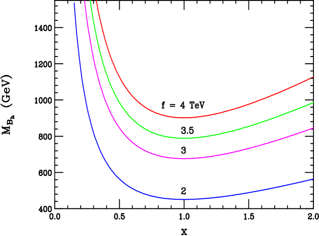
Figure 1: The theoretical predictions for the mass of the gauge boson $B_{h}$ as a function of $x=g^{{}^{\prime}}_{t}/g^{{}^{\prime}}$, the ratio of its coupling relative to the corresponding SM coupling, for several values of the scale $f$.

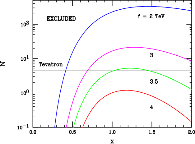
Figure 2: The expected number of Drell-Yan events from the production of the $B_{h}$ boson during Tevatron Run I (110 ${\rm pb}^{-1}$) as a function of $x=g^{{}^{\prime}}_{t}/g^{{}^{\prime}}$, the ratio of its coupling relative to the corresponding SM coupling, for several values of $f$. The horizontal line represents the 95% CL bound from CDF [11] for this mechanism; the parameter region above this line is excluded.

We now analyze the constraints arising from EW precision data. The new parameters introduced in this model are the scale $f$ (or the ratio $\delta=\nu/f$), the couplings $g_{t}$ and $h_{t}$, and the top quark sector mixing angle $\theta_{t}$, which enters both $\delta\rho$ and $Z$-pole $b$-quark observables through the loop corrections discussed in the previous section. Rather than perform a combined fit to all four quantities, we study a series of two-dimensional $\chi^{2}$ fits for various combinations of parameters; this is sufficient to illustrate the essential physics. In deriving our constraints we follow the analysis of [16]; we calibrate our fits by first varying the Higgs boson mass until we find the $\chi^{2}$ value that reproduces the 95% CL upper bound on $m_{H}$ presented in  [1]. We then use this reference $\chi^{2}$ to determine whether a given set of model parameters provides a good fit to the EW data. We say that a set of parameters is disallowed if the resulting $\chi^{2}$ exceeds this reference value. We will first consider the observables $m_{W}$, $\Gamma_{l}$, $s_{W,eff}^{2,lep}$, $N_{\nu}$, $R_{b}$, $A_{b}$, $R_{c}$, and $A_{c}$, and later will include $s_{W,N}^{2,os}$ as determined from NuTeV. The error correlation between these measurements is quite small [1], and will be neglected in our analysis. We use ZFITTER [14] to derive the SM predictions for these quantities.

We first set $g_{t}=g$ and $g^{{}^{\prime}}_{t}=g^{{}^{\prime}}$, and vary both ${\rm sin}\left(\theta_{t}\right)$ and $\delta$. The results of this fit for both $m_{H}=115$ GeV and $m_{H}=200$ GeV are shown in Fig. 3; the shaded region is allowed by the EW fit at the 95% CL, while the remainder is excluded. Although $m_{H}=200$ GeV is allowed in this model, unlike in the SM where $m_{H}<193$ GeV at the 95% CL, only a small sliver near the boundary $\delta/\sqrt{2}={\rm tan}\left(\theta_{t}\right)$ satisfies the EW precision constraints. This region persists but shrinks for larger values of $m_{H}$. The tail along this boundary for large values of $\delta$ is primarily due to the $t$ and $t^{{}^{\prime}}$ mixing contributions to $\delta\rho$. We see that the Tevatron constraints are quite significant here, as they completely exclude this region. Included in these figures are curves representing the predictions for several $t^{{}^{\prime}}$ masses as functions of $\delta$ and ${\rm sin}\left(\theta_{t}\right)$ from Eq. 22. We see that the Tevatron limit requires that $m_{t^{{}^{\prime}}}>7$ TeV, which is significantly larger than the naturalness bound $m_{t^{{}^{\prime}}}<2$ TeV. This is beyond the range for direct discovery at the LHC.

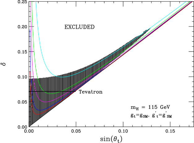
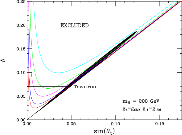
Figure 3: Fit to the EW precision data varying ${\rm sin}\left(\theta_{t}\right)$ and $\delta$, for $m_{H}=115$ GeV (upper) and $m_{H}=200$ GeV (lower). The diagonal line indicates the bound $\delta/\sqrt{2}\leq{\rm tan}\left(\theta_{t}\right)$, the horizontal line denotes the 95% CL bound from $B_{h}$ production at the Tevatron. The series of curved lines indicates the $t^{{}^{\prime}}$ mass $m_{t^{{}^{\prime}}}$ as a function of $\delta$ and ${\rm sin}\left(\theta_{t}\right)$; from top to bottom, they represent $m_{t^{{}^{\prime}}}=5$, 7.5, 10, 15, and 20 TeV. The shaded regions are allowed by the EW fit. For the remainder of our discussion, we label $g$ and $g^{\prime}$ as $g_{SM}$ and $g^{\prime}_{SM}$, respectively, in the figures.

We now study the case where the couplings $g_{t}$ and $g^{{}^{\prime}}_{t}$ are varied within natural ranges away from their corresponding SM values. For this and all later discussions we assume $m_{H}=115$ GeV. Shown in Fig. 4 are the results of the EW fits for the following four coupling choices: (1) $g_{t}=g$ and $g^{{}^{\prime}}_{t}=g^{{}^{\prime}}/2$; (2) $g_{t}=g$ and $g^{{}^{\prime}}_{t}=2g^{{}^{\prime}}$; (3) $g_{t}=g/2$ and $g^{{}^{\prime}}_{t}=g^{{}^{\prime}}$; (4) $g_{t}=g/4$ and $g^{{}^{\prime}}_{t}=g^{{}^{\prime}}$. We see from the top two figures that the EW constraints are strongest in the case where the Tevatron constraints are weakened. As can be seen from Fig. 2, the Tevatron limits are the most stringent when $g^{{}^{\prime}}_{t}/g^{{}^{\prime}}\approx 1$, and decrease away from this region. This region is exactly where $\delta\rho_{G}$ vanishes, as can be seen from Eq. 2; away from this point the contribution of $\delta\rho$ to the EW fit becomes more important. For case (1), the EW precision constraints require $f\mathrel{\mathchoice{\lower 3.01385pt\vbox{\halign{$\matth\displaystyle\hfil#\hfil$\cr>\crcr\sim\crcr}}}{\lower 3.01385pt\vbox{\halign{$\matth\textstyle\hfil#\hfil$\cr>\crcr\sim\crcr}}}{\lower 3.01385pt\vbox{\halign{$\matth\scriptstyle\hfil#\hfil$\cr>\crcr\sim\crcr}}}{\lower 3.01385pt\vbox{\halign{$\matth\scriptscriptstyle\hfil#\hfil$\cr>\crcr\sim\crcr}}}}3.5$ TeV, while in case (2) this bound is strengthened to $f\mathrel{\mathchoice{\lower 3.01385pt\vbox{\halign{$\matth\displaystyle\hfil#\hfil$\cr>\crcr\sim\crcr}}}{\lower 3.01385pt\vbox{\halign{$\matth\textstyle\hfil#\hfil$\cr>\crcr\sim\crcr}}}{\lower 3.01385pt\vbox{\halign{$\matth\scriptstyle\hfil#\hfil$\cr>\crcr\sim\crcr}}}{\lower 3.01385pt\vbox{\halign{$\matth\scriptscriptstyle\hfil#\hfil$\cr>\crcr\sim\crcr}}}}7.2$ TeV. These correspond to limits of $m_{t^{{}^{\prime}}}>7$ TeV and $m_{t^{{}^{\prime}}}>14$ TeV, respectively. The strongest constraints for cases (3) and (4) arise from the Tevatron direct searches; the EW precision constraints are relatively weak for these parameter choices. To further demonstrate that bounds from EW data become strong in precisely those regions in which the Tevatron constraints decrease, we present in Fig. 5 the results of fits where we set $f=2$ TeV and vary both ${\rm sin}\left(\theta_{t}\right)$ and $x$. The three fits we perform use the following definitions of $x$: (1) $g_{t}=xg$ and $g^{{}^{\prime}}_{t}=xg^{{}^{\prime}}$; (2) $g_{t}=xg/2$ and $g^{{}^{\prime}}_{t}=xg^{{}^{\prime}}$; (3) $g_{t}=xg$ and $g^{{}^{\prime}}_{t}=xg^{{}^{\prime}}/2$. These variations in the couplings within natural ranges provide for a thorough exploration of the model parameter space. In all three cases the parameter values allowed by the EW fit are clustered very near $g^{{}^{\prime}}_{t}=g^{{}^{\prime}}$, and are excluded by the Tevatron constraints. We obtain identical results if we choose $f=3$ TeV. Combining the results of these fits, we can conclude that $f\mathrel{\mathchoice{\lower 3.01385pt\vbox{\halign{$\matth\displaystyle\hfil#\hfil$\cr>\crcr\sim\crcr}}}{\lower 3.01385pt\vbox{\halign{$\matth\textstyle\hfil#\hfil$\cr>\crcr\sim\crcr}}}{\lower 3.01385pt\vbox{\halign{$\matth\scriptstyle\hfil#\hfil$\cr>\crcr\sim\crcr}}}{\lower 3.01385pt\vbox{\halign{$\matth\scriptscriptstyle\hfil#\hfil$\cr>\crcr\sim\crcr}}}}3.5$ TeV throughout the full parameter space of the model. This implies a minimum mass of $m_{t^{{}^{\prime}}}=7$ TeV for the $t^{{}^{\prime}}$ state, which is beyond the reach of the LHC.

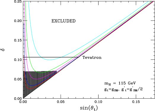
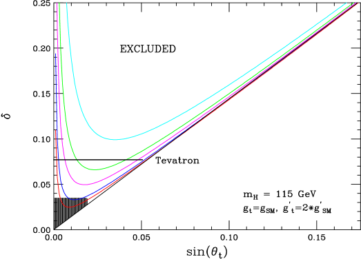
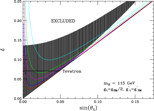
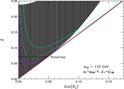
Figure 4: Fit to the EW precision data varying ${\rm sin}\left(\theta_{t}\right)$ and $\delta$, for various choices of $g_{t}$ and $g_{t^{{}^{\prime}}}$ as indicated. The diagonal line represents the bound $\delta/\sqrt{2}\leq{\rm tan}\left(\theta_{t}\right)$, the horizontal line denotes the 95% CL bound from $B_{h}$ production at the Tevatron, and the series of curved lines corresponds to the $t^{{}^{\prime}}$ mass $m_{t^{{}^{\prime}}}$ as a function of $\delta$ and ${\rm sin}\left(\theta_{t}\right)$; from top to bottom, they represent $m_{t^{{}^{\prime}}}=5$, 7.5, 10, 15, and 20 TeV. The shaded regions are allowed by the EW fit.

Figure 5: Fit to the EW precision data varying both ${\rm sin}\left(\theta_{t}\right)$ and $x$, for $f=2$ TeV. The shaded regions are allowed by the EW fit, while the areas above the horizontal lines are forbidden by Tevatron direct search constraints. The rightmost boundary of the figure is determined by the constraint $\delta/\sqrt{2}\leq{\rm tan}\left(\theta_{t}\right)$.

Having established that $f\mathrel{\mathchoice{\lower 3.01385pt\vbox{\halign{$\matth\displaystyle\hfil#\hfil$\cr<\crcr\sim\crcr}}}{\lower 3.01385pt\vbox{\halign{$\matth\textstyle\hfil#\hfil$\cr<\crcr\sim\crcr}}}{\lower 3.01385pt\vbox{\halign{$\matth\scriptstyle\hfil#\hfil$\cr<\crcr\sim\crcr}}}{\lower 3.01385pt\vbox{\halign{$\matth\scriptscriptstyle\hfil#\hfil$\cr<\crcr\sim\crcr}}}}3.5$ is excluded by the data, we now set $f=4$ TeV, which is allowed by both EW precision constraints and Tevatron direct search limits. We study the fit to the EW precision data as we vary both ${\rm sin}\left(\theta_{t}\right)$ and $x$; we choose the same three cases for the relations of the couplings as examined above. The results of these fits are presented in Fig. 6. We see that a far larger region of the coupling space is consistent with the data in this case, and that the EW data allows significant deviations from the $g^{{}^{\prime}}_{t}=g^{{}^{\prime}}$ limit. To examine the contributions of the various observables to the fit, we present in Fig. 7 the $\Delta\chi^{2}$ values for the various observables obtained in the $g_{t}=xg$, $g^{{}^{\prime}}_{t}=xg^{{}^{\prime}}$ fit; $\Delta\chi^{2}$ is the difference between the $\chi^{2}$ values obtained in the Littlest Higgs model and in the SM. Included in these figures are all values of $x$ which satisfy the bounds imposed by the EW data. We have not presented our results for the observables $R_{c}$, $A_{c}$, and $A_{b}$ because their $\Delta\chi^{2}$ values are very nearly zero throughout the entire parameter space; i.e., they have no influence on the fit. All of the $\Delta\chi^{2}$ ranges exhibit a dip either upwards or downwards at the right edge of these figures. These arise from the $t$ and $t^{{}^{\prime}}$ contributions to either $\delta\rho$ or, for $R_{b}$, the $Z\bar{b}b$ vertex. Although $m_{t^{{}^{\prime}}}$ becomes large as ${\rm sin}\left(\theta_{t}\right)\rightarrow\delta/\sqrt{2}$, since the $t^{{}^{\prime}}$ mixes with the top quark it does not decouple, in the sense discussed above, for some parameter space regions. We see that $M_{W}$ is generally better predicted by the Littlest Higgs model than the SM; this remains true for other parameter choices. The shift in $M_{W}$ depends only on the coupling of the fermions to the $SU(2)_{1}$ gauge bosons, and not on their coupling to the hypercharge bosons; this will therefore remain true for other choices of fermion transformation assignments. We also see that while $R_{b}$ is not affected until ${\rm sin}\left(\theta_{t}\right)\rightarrow\delta/\sqrt{2}$, both $\Gamma_{l}$ and $s_{W,eff}^{2,lep}$ are very sensitive to the deviations predicted by the Littlest Higgs, and that the agreement between the predicted values for these observables and the experimental measurements is always worse than in the SM.

Figure 6: Fit to the EW precision data varying both ${\rm sin}\left(\theta_{t}\right)$ and $x$, for $f=4$ TeV. The shaded regions are allowed by the EW fit. The rightmost boundary of the figure is determined by the constraint $\delta/\sqrt{2}\leq{\rm tan}\left(\theta_{t}\right)$.

Figure 7: The $\Delta\chi^{2}$ values for several observables as functions of ${\rm sin}\left(\theta_{t}\right)$ for the case $g_{t}=xg$ and $g^{{}^{\prime}}_{t}=xg^{{}^{\prime}}$; included are all $x$ values that satisfy the precision EW constraints as shown in the previous figure.

Finally, we discuss the effect on the fit of the NuTeV measurement of the on-shell value of the weak mixing angle $s_{W,N}^{2,os}$. The NuTeV result currently disagrees with that derived from $Z$-pole data by approximately 3 standard deviations [15]. Although this is possibly a signal of new physics, several more mundane explanations, such as larger parton distribution function uncertainties than those assumed by the NuTeV collaboration, asymmetric strange and charm sea quark distributions, or nuclear effects, have been suggested [17]. With this caveat in mind, we will assume both the central value and error determined by the NuTeV collaboration, and repeat our analysis including the NuTeV result. To demonstrate that the allowed range of $f$ is unaffected by the inclusion of the NuTeV measurement, we display the results of re-performing the following two analyses in Fig. 8: (1) varying $\delta$ and ${\rm sin}\left(\theta_{t}\right)$ while setting $g_{t}=g$ and $g^{{}^{\prime}}_{t}=g^{{}^{\prime}}$, the analog of the fit presented in Fig. 3; (2) varying ${\rm sin}\left(\theta_{t}\right)$ and $x$ with $f=2$ TeV, and $x$ defined by $g_{t}=xg$ and $g^{{}^{\prime}}_{t}=xg^{{}^{\prime}}$, the analog of the result shown in Fig. 5. Comparing these figures with those presented previously, we see that the constraint on $f$ is unchanged by the addition of the NuTeV data. Although the full EW data set allows a slightly larger range of parameters here than before, the Tevatron constraint again excludes these regions. For other coupling choices, the NuTeV measurement again either very slightly increases or decreases the size of the allowed parameter space; no large swath of new parameter values are allowed.

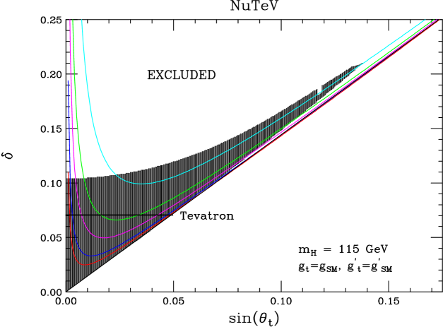
Figure 8: Fit to the EW precision data including the NuTeV measurement of the on-shell weak mixing angle. The top figure studies the variation with $\delta$ and ${\rm sin}\left(\theta_{t}\right)$, while the lower figure shows the dependence on ${\rm sin}\left(\theta_{t}\right)$ and $x$ with $f=2$ TeV.

We next set $f=4$ TeV, $g_{t}=xg$ and $g^{{}^{\prime}}_{t}=xg^{{}^{\prime}}$, and vary both ${\rm sin}\left(\theta_{t}\right)$ and $x$; the results are presented in Fig. 9. We display the allowed region in the $x-\sin(\theta_{t})$ plane as well as the values of $\Delta\chi^{2}$ for $s_{W,N}^{2,os}$. The Littlest Higgs model shifts $s_{W,N}^{2,os}$ in the direction preferred by the NuTeV measurement throughout most of the entire parameter space; this remains true for other choices of the couplings. The size of the allowed region is smaller than in the case where the NuTeV data is not included. The shifts induced by the Littlest Higgs model ($\approx 0.5-1.5$ $\sigma$) cannot compensate for the large $\approx 3$ $\sigma$ deviation of the SM prediction from the NuTeV results.

Figure 9: Fit to the EW precision data including the NuTeV measurement of the on-shell weak mixing angle; we have set $f=4$ TeV and $g_{t}=xg$, $g^{{}^{\prime}}_{t}=xg^{{}^{\prime}}$. The top figure shows the fit to the EW data, while the lower figure illustrates the $\chi^{2}$ shift from the SM for those values of $x$ and ${\rm sin}\left(\theta_{t}\right)$ which satisfy the EW constraints.

Before concluding we note that we have not discussed the possible influence of measurements of Atomic Parity Violation (APV) on the fits. Until recently the experimental value of the weak charge, $Q_{W}$, differed from the predictions of the SM by about $2\sigma$ [18]. After a series of detailed theoretical calculations including various atomic effects it now seems that experiment and theoretical predictions are in agreement [19]. However, since the theoretical calculation of $Q_{W}$ may still be in flux we do not include this observable in our fits. After computing the corrections to $Q_{W}$ in this model and scanning the allowed regions from our previous fits, we find that either sign for the shift of $Q_{W}$ can be generated.

4 Conclusions

Little Higgs models are a novel attempt to address the hierarchy problem. These theories predict the existence of a host of new particles at the TeV scale, which are necessary to cancel the quadratic divergences of the Standard Model. Here, we have examined the simplest version of these models, the Littlest Higgs, which contains four new gauge bosons, a weak isosinglet quark, $t^{\prime}$, with $Q=2/3$, as well as an isotriplet scalar field with their masses being constrained by naturalness requirements. In this paper, we have considered the contributions of these new states to precision electroweak observables, and have examined the additional constraints provided by the direct searches for new particles at the Tevatron. We have performed a thorough exploration of the parameter space of this model and have found that there are small regions allowed by the precision data where the parameters take on their natural values. When the additional limits provided by the Tevaton are included, these regions are no longer permitted. By combining the direct and indirect effects of these new states we have constrained the ‘decay constant’$f$ to rather large values $\mathrel{\mathchoice{\lower 3.01385pt\vbox{\halign{$\matth\displaystyle\hfil#\hfil$\cr>\crcr\sim\crcr}}}{\lower 3.01385pt\vbox{\halign{$\matth\textstyle\hfil#\hfil$\cr>\crcr\sim\crcr}}}{\lower 3.01385pt\vbox{\halign{$\matth\scriptstyle\hfil#\hfil$\cr>\crcr\sim\crcr}}}{\lower 3.01385pt\vbox{\halign{$\matth\scriptscriptstyle\hfil#\hfil$\cr>\crcr\sim\crcr}}}}3.5$ TeV; similarly, to satisfy both sets of data $m_{t^{\prime}}\mathrel{\mathchoice{\lower 3.01385pt\vbox{\halign{$\matth\displaystyle\hfil#\hfil$\cr>\crcr\sim\crcr}}}{\lower 3.01385pt\vbox{\halign{$\matth\textstyle\hfil#\hfil$\cr>\crcr\sim\crcr}}}{\lower 3.01385pt\vbox{\halign{$\matth\scriptstyle\hfil#\hfil$\cr>\crcr\sim\crcr}}}{\lower 3.01385pt\vbox{\halign{$\matth\scriptscriptstyle\hfil#\hfil$\cr>\crcr\sim\crcr}}}}7$ TeV which is far beyond the reach of direct searches at the LHC. These bounds imply that significant fine-tuning must be present in order for this model to resolve the hierarchy. We thus find that the Littlest Higgs model is tightly constrained by the combination of precision electroweak data and direct Tevatron searches.

Acknowledgements

The authors would like to thank Nima Arkani-Hamed, Gustavo Burdman, Alex Kagan, Ann Nelson, Michael Peskin, Aaron Pierce and Jay Wacker for useful discussions related to this work.

Note Added: A related work [20], which studied the effects of mixing in the gauge sector in the Littlest Higgs model, appeared while this paper was being completed.

Appendix A

Here we investigate the effects of the scalar triplet vev on the precision electroweak observables. The vev gives a negative contribution to the $\rho$-parameter which can be written as

$$\delta\rho_{\phi}=-{\delta^{2}\over 4}\left[{2\lambda g_{t}^{2}\over a(g^{2}+g_{t}^{2})^{2}}-1\right]^{2}\,,$$ (39)

where $\lambda$ is the Higgs quartic coupling, which can be expressed in terms of the Higgs mass via [21]

$$\lambda\sim{1\over 3}\left[{m_{h}\over 200~{}{\rm GeV}}\right]^{2}\,.$$ (40)

$a$ represents a new parameter arising from the coefficient of an ultra-violet operator; naturalness suggests that the value of $a$ lies in the range $0.1-1.0$. Including this contribution in the fit to the global electroweak data set (minus the NuTeV measurement) yields the results displayed in Fig. 10. Here, we have examined the previously least restrictive case, as observed from Fig. 4, and set the values of the couplings to $g_{t}=g/4$, $g_{t}^{\prime}=g^{\prime}$, while varying the parameter $a$. For comparison, we also show our previous results for the case when the contributions from the triplet vev are not included. We see that the addition of the contribution from the triplet vev only worsens the ability of this model to accomodate the electroweak data set. We have checked that the constraints become even more restrictive as $a$ approaches unity, and as the value of the Higgs mass increases.

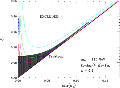
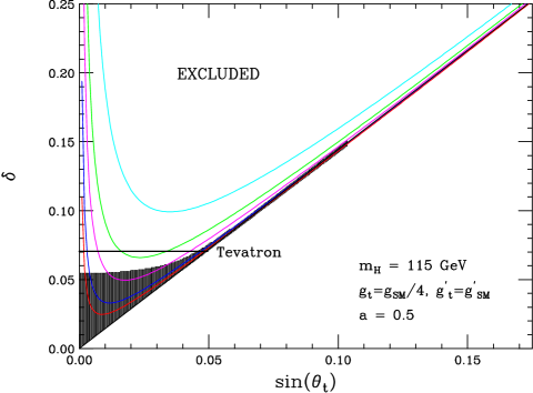
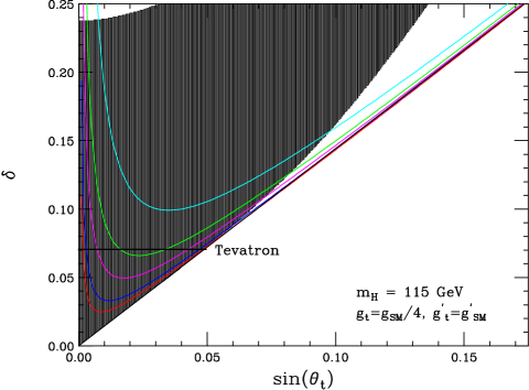
Figure 10: Results from the global fit to the electroweak precision data, including the contributions from the scalar triplet vev to the electroweak observables for various values of the parameter $a$. Also shown are the results from the fit when the triplet vev is not included. The horizontal line denotes the 95% CL bound from $B_{h}$ production at the Tevatron, and the series of curved lines corresponds to the $t^{\prime}$ mass $m_{t^{\prime}}$ as a function of $\delta$ and $\sin(\theta_{t})$; from top to bottom they represent $m_{t^{\prime}}=2.5,\,5,\,7.5,$  and 10 TeV. The shaded regions are allowed by the EW fit.

Appendix B

We define here the loop integrals in Eq. 35 which arise in the computation of the shift in $\delta g^{b}_{L}$ due to the vertex correction diagrams containing $t$ and $t^{{}^{\prime}}$ states:

$$I_{1}\left(m_{i},m_{j}\right) = \int_{0}^{1}dx\int_{0}^{1-x}dy\frac{m_{i}m_{j}}{\left(1-x-y\right)M_{W}^{2}-xyM_{Z}^{2}+xm_{i}^{2}+ym_{j}^{2}}\,\,,$$

$$I_{2}\left(m_{i},m_{j}\right) = \int_{0}^{1}dx\int_{0}^{1-x}dy\,{\rm ln}\left[\frac{\left(1-x-y\right)M_{W}^{2}-xyM_{Z}^{2}+xm_{i}^{2}+ym_{j}^{2}}{\mu^{2}}\right]\,\,,$$

$$I_{3}\left(m_{i}\right) = \int_{0}^{1}dx\int_{0}^{1-x}dy\,{\rm ln}\left[\frac{\left(1-y\right)M_{W}^{2}-x\left(1-x-y\right)M_{Z}^{2}+ym_{i}^{2}}{\mu^{2}}\right]\,\,,$$

$$I_{4}\left(m_{i}\right) = \int_{0}^{1}dx\,x\,{\rm ln}\left[\frac{xM_{W}^{2}+\left(1-x\right)m_{i}^{2}}{\mu^{2}}\right]\,\,,$$ (41)

where $\mu$ is an arbitrary renormalization scale that cancels from the final expression after all the individual diagrams are summed over.

References

• [1] M. Grünewald, talk presented at 31st International Conference On High Energy Physics, Amsterdam, Netherlands, July 2002; LEP/SLD Electroweak Working Group, LEPEWWG/2002-01.
• [2] M. E. Peskin and J. D. Wells, Phys. Rev. D 64, 093003 (2001) [arXiv:hep-ph/0101342].
• [3] H. E. Haber and G. L. Kane, Phys. Rept.  117, 75 (1985).
• [4] N. Arkani-Hamed, S. Dimopoulos and G. R. Dvali, Phys. Lett. B 429, 263 (1998) [arXiv:hep-ph/9803315], and Phys. Rev. D 59, 086004 (1999) [arXiv:hep-ph/9807344]; I. Antoniadis, N. Arkani-Hamed, S. Dimopoulos and G. R. Dvali, Phys. Lett. B 436, 257 (1998) [arXiv:hep-ph/9804398]; L. Randall and R. Sundrum, Phys. Rev. Lett.  83, 3370 (1999) [arXiv:hep-ph/9905221], and Phys. Rev. Lett.  83, 4690 (1999) [arXiv:hep-th/9906064].
• [5] For a review, see, J. Hewett and M. Spiropulu, arXiv:hep-ph/0205106.
• [6] N. Arkani-Hamed, A. G. Cohen, E. Katz and A. E. Nelson, JHEP 0207, 034 (2002) [arXiv:hep-ph/0206021].
• [7] N. Arkani-Hamed, A. G. Cohen, E. Katz, A. E. Nelson, T. Gregoire and J. G. Wacker, JHEP 0208, 021 (2002) [arXiv:hep-ph/0206020]; T. Gregoire and J. G. Wacker, JHEP 0208, 019 (2002) [arXiv:hep-ph/0206023]; I. Low, W. Skiba and D. Smith, Phys. Rev. D 66, 072001 (2002) [arXiv:hep-ph/0207243].
• [8] H. Georgi and A. Pais, Phys. Rev. D 10, 539 (1974), and Phys. Rev. D 12, 508 (1975); D. B. Kaplan and H. Georgi, Phys. Lett. B 136, 183 (1984); D. B. Kaplan, H. Georgi and S. Dimopoulos, Phys. Lett. B 136, 187 (1984); H. Georgi, D. B. Kaplan and P. Galison, Phys. Lett. B 143, 152 (1984); H. Georgi and D. B. Kaplan, Phys. Lett. B 145, 216 (1984); M. J. Dugan, H. Georgi and D. B. Kaplan, Nucl. Phys. B 254, 299 (1985).
• [9] N. Arkani-Hamed, A. G. Cohen and H. Georgi, Phys. Rev. Lett.  86, 4757 (2001) [arXiv:hep-th/0104005]; C. T. Hill, S. Pokorski and J. Wang, Phys. Rev. D 64, 105005 (2001) [arXiv:hep-th/0104035]; N. Arkani-Hamed, A. G. Cohen and H. Georgi, Phys. Lett. B 513, 232 (2001) [arXiv:hep-ph/0105239]; H. C. Cheng, C. T. Hill and J. Wang, Phys. Rev. D 64, 095003 (2001) [arXiv:hep-ph/0105323].
• [10] N. Arkani-Hamed, A. G. Cohen, T. Gregoire and J. G. Wacker, JHEP 0208, 020 (2002) [arXiv:hep-ph/0202089]; K. Lane, Phys. Rev. D 65, 115001 (2002) [arXiv:hep-ph/0202093]; R. S. Chivukula, N. Evans and E. H. Simmons, Phys. Rev. D 66, 035008 (2002) [arXiv:hep-ph/0204193].
• [11] F. Abe et al., CDF Collaboration, Phys. Rev. Lett. 79, 2191 (1997).
• [12] See, for example, H. Georgi and D. B. Kaplan, Phys. Lett. B 145, 216 (1984) in Ref. [8].
• [13] K. Hagiwara et al. [Particle Data Group Collaboration], Phys. Rev. D 66, 010001 (2002).
• [14] D. Y. Bardin, P. Christova, M. Jack, L. Kalinovskaya, A. Olchevski, S. Riemann and T. Riemann, in Comput. Phys. Commun.  133, 229 (2001) [arXiv:hep-ph/9908433].
• [15] G. P. Zeller et al. [NuTeV Collaboration], Phys. Rev. Lett.  88, 091802 (2002) [arXiv:hep-ex/0110059].
• [16] T. G. Rizzo and J. D. Wells, Phys. Rev. D 61, 016007 (2000) [arXiv:hep-ph/9906234].
• [17] For a discussion of these points, see: S. Davidson, S. Forte, P. Gambino, N. Rius and A. Strumia, JHEP 0202, 037 (2002) [arXiv:hep-ph/0112302]; G. P. Zeller et al. [NuTeV Collaboration], Phys. Rev. D 65, 111103 (2002) [arXiv:hep-ex/0203004]; P. Gambino, arXiv:hep-ph/0211009.
• [18] S. C. Bennett and C. E. Wieman, Phys. Rev. Lett.  82, 2484 (1999) [arXiv:hep-ex/9903022].
• [19] M. Y. Kuchiev and V. V. Flambaum, arXiv:hep-ph/0206124.
• [20] C. Csaki, J. Hubisz, G. D. Kribs, P. Meade and J. Terning, arXiv:hep-ph/0211124.
• [21] N. Arkani-Hamed, private communication. The scalar triplet contribution to $\Delta\rho$ is also derived in Ref. [20].