Testing of CP, CPT and causality violation with the light propagation in vacuum in presence of the uniform electric and magnetic fields.

Abstract

We have considered the structure of the fundamental symmetry violating part of the photon refractive index in vacuum in the presence of constant electric and magnetic fields. This part of the refractive index can, in principle, contain CPT symmetry breaking terms. Some of the terms violate Lorentz invariance, whereas the others violate locality and causality. Estimates of these effects, using laser experiments are considered.

I Introduction

Recently, the experiments on searching for the birefringence of a vacuum have been carried out and planed camer ; pvlas ; bmv . The BMV project bmv was proposed to achieve an accuracy sufficient for detection of vacuum birefringence, predicted by QED. In addition, search for exotic non QED interactions is possible in such experiments. In this article we discuss what kinds of discrete, i.e., P, T, C symmetries breaking terms can be present in the photon refractive index in vacuum in constant electric and magnetic fields.

CP symmetry breaking in $K$- meson cronin , and $B$-meson babar decays, as well as time reversal symmetry violation in $K_{0}-\bar{K}_{0}$ oscillations cplear can be currently described by the standard model with the Cabibbo-Kobayashi-Maskawa matrix. It would be interesting to find CP violation in the other systems, different from the $K_{0}$ or $B_{0}$. It would be especially interesting to find some violation of the unconquerable CPT symmetry. No signals for CPT violation have been observed yet despite numerous experimental tests.

From the CPT theorem streater we know, that CPT invariance of some field theory follows from locality and invariance under Lorenz transforms. Usually CPT violation is considered to be due to breaking of Lorentz invariance kostel . However, it is possible, that locality is the less fundamental requirement, than Lorentz invariance, therefore, experiments searching for CPT violation of both types are of interest.

II Electromagnetic wave in vacuum in constant electric and magnetic fields.

Let us consider the propagation of an electromagnetic wave in vacuum in the presence of uniform constant electric and magnetic fields. Since a photon has no electric charge, such a medium is a medium with constant refractive index. We will assume that the field of the electromagnetic wave obeys the Maxwell equation $\frac{\partial F^{\mu\nu}(x)}{\partial x^{\nu}}=-4\pi j^{\mu}(x)$, where $j(x)$ is a current of all the particles, which can interact with the photons. The current arises due to vacuum polarization by the electromagnetic wave in presence of the external fields. Assuming that the wave field is weak and vacuum in the homogeneous external field remains homogeneous, we can, in the general case, express the current linearly through the four-potential of the wave field:

$$j^{\mu}(x)=-\int{\mathcal{P}}^{\mu\nu}(x-x^{\prime})A_{\nu}(x^{\prime})d^{4}x^{\prime},$$ (1)

where ${\mathcal{P}}^{\mu\nu}(x)$ is some tensor. We do not consider the case of the strong external electric field, when vacuum instability frad should be taken into account. After Fourier transforms of the four-current $j(x)=\int j(k)e^{-ikx}d^{4}k$ and four-potential of the electromagnetic field $A(x)=\int A(k)e^{-ikx}d^{4}k$ the Maxwell equation is rewritten as

$$k^{2}A^{\mu}(k)-k^{\mu}(kA)=-j^{\mu}(k),$$ (2)

where

$$j^{\mu}(k)=-{\mathcal{P}}^{\mu\nu}(k)A_{\nu}(k).$$ (3)

The four-tensor ${\mathcal{P}}^{\mu\nu}(k)=\int{\mathcal{P}}^{\mu\nu}(x)e^{ikx}d^{4}x$ should be constructed from the tensor of the external field ${\mathcal{F}}^{\mu\nu}$ and a photon wave vector $k$, since only they are available. By virtue of the gauge invariance and current conservation the relations ${\mathcal{P}}^{\mu\nu}k_{\nu}=k_{\mu}{\mathcal{P}}^{\mu\nu}=0$ must be imposed on ${\mathcal{P}}^{\mu\nu}$.

It is also necessary to emphasize, that all the possible interactions are supposed to be small, so $k^{2}$ can be set to zero on the right-hand side of Maxwell’s equation during evaluation of ${\mathcal{P}}^{\mu\nu}$; in addition, only that part of ${\mathcal{P}}^{\mu\nu}$ should be taken into account which does not become zero when acting on the four-vector polarization $e_{\mu}(k)$ of a real photon (for real photons $k^{\mu}e_{\mu}=0$ ). The structure of the polarization operator, including off mass shell terms was considered in Ref. shabad for the case when all the symmetries are conserved and is considered in APPENDIX A for the case of symmetry violation.

In Eqs. (2) and (3) the gauge is not fixed yet. We shall choose the gauge with the null component of the four-potential being equal to zero: $\phi=0$. Then $\bm{E}=-\frac{\partial\bm{A}}{\partial t}$ and $\bm{E}(\bm{k},\omega)=i\omega\bm{A}$. In a given gauge we obtain from Eqs. (2) and (3):

$$\bm{k}^{2}E^{i}-k^{i}(\bm{k}\bm{E})-\omega^{2}\left(\delta^{ij}+\frac{{\mathcal{P}}^{ij}}{\omega^{2}}\right)E^{j}=0,$$ (4)

where the three-dimensional tensor ${\mathcal{P}}^{ij}$ is the spatial part of the four-tensor ${\mathcal{P}}^{\mu\nu}$. Equation (4) shows, that $\varepsilon^{ij}=\delta^{ij}+\frac{{\mathcal{P}}^{ij}}{\omega^{2}}$, plays the role of the product of the dielectric and magnetic constants the vacuum in an external field. Further, for short, we shall simply call it the dielectric constant $\varepsilon^{ij}$ of vacuum in the external fields.

Let us consider the structure of the four-tensor ${\mathcal{P}}^{\mu\nu}$ in detail. It can be presented as an expansion in orders of the external field. Provided the requirements ${\mathcal{P}}^{\mu\nu}k_{\nu}=k_{\mu}{\mathcal{P}}^{\mu\nu}=0$ footnote1 , and $e_{\mu}^{*\prime}{\mathcal{P}}^{\mu\nu}e^{\nu}\neq 0$, $k^{2}=0$ are met, and in the second order in the external field tensor ${\mathcal{F}}^{\mu\nu}$ we obtain:

$${\mathcal{P}}^{\mu\nu}=a_{1}\,{\mathcal{F}}^{\mu\alpha}k_{\alpha}{\mathcal{F}}^{\nu\sigma}k_{\sigma}+a_{2}\,e^{\mu\lambda\varrho\sigma}{\mathcal{F}}_{\lambda\varrho}k_{\sigma}e^{\nu\phi\delta\alpha}{\mathcal{F}}_{\phi\delta}k_{\alpha}+i\,b_{1}\,e^{\mu\nu\alpha\beta}k_{\alpha}{\mathcal{F}}_{\beta\varrho}{\mathcal{F}}^{\varrho\phi}k_{\phi}$$

$$+c_{1}(e^{\mu\lambda\varrho\sigma}{\mathcal{F}}_{\lambda\varrho}k_{\sigma}{\mathcal{F}}^{\nu\delta}k_{\delta}+e^{\nu\lambda\varrho\sigma}{\mathcal{F}}_{\lambda\varrho}k_{\sigma}{\mathcal{F}}^{\mu\delta}k_{\delta}).$$ (5)

Equation (5) is valid when the external field is slowly varying with respect to the wavelength of the photon; further terms involving derivatives of the external field should be included.

The quantity $e^{*\prime}_{\mu}{\mathcal{P}}^{\mu\nu}e_{\nu}$ is similar to the invariant forward photon scattering amplitude in the external field. Let us find out its properties under CPT transformation. Under C, P and T transforms the tensor of the external field, wave four-vector and four-polarization of the photon are changed as lan4

$$T{\mathcal{F}}^{\mu\nu}\rightarrow-{\mathcal{F}}_{\mu\nu}~{}~{}~{}Tk^{\mu}\rightarrow k_{\mu}~{}~{}~{}Te^{\mu}\rightarrow e^{*\prime}_{\mu}~{}~{}~{}Te^{*\prime}_{\mu}\rightarrow e^{\mu}$$

$$C{\mathcal{F}}^{\mu\nu}\rightarrow-{\mathcal{F}}^{\mu\nu}~{}~{}~{}Ck^{\mu}\rightarrow k^{\mu}~{}~{}~{}Ce^{\mu}\rightarrow-e^{\mu}~{}~{}~{}~{}~{}~{}~{}~{}~{}~{}~{}~{}~{}~{}$$

$$P{\mathcal{F}}^{\mu\nu}\rightarrow{\mathcal{F}}_{\mu\nu}~{}~{}~{}Pk^{\mu}\rightarrow k_{\mu}~{}~{}~{}Pe^{\mu}\rightarrow e_{\mu}.~{}~{}~{}~{}~{}~{}~{}~{}~{}~{}~{}~{}~{}~{}~{}~{}~{}~{}$$ (6)

Hence, ${\mathcal{P}}^{\mu\nu}$ should be symmetric to satisfy CPT invariance. The term proportional to $b_{1}$ breaks CPT invariance with parity breaking only. The term, proportional to $c_{1}$, is CPT invariant, but P-, CP- and T-violating. The terms proportional to $a_{1}=\frac{16}{45}\frac{\alpha^{2}}{m^{4}}\approx 2.78\times 10^{-4}~{}\mbox{MeV}^{-4}$ and $a_{2}=\frac{7}{45}\frac{\alpha^{2}}{m^{4}}\approx 1.21\times 10^{-4}~{}\mbox{MeV}^{-4}$ arise in the framework of conventional QED adler ; lan4 . Here $\alpha$ is fine structure constant and $m$ is the electron mass. From Eq. (5) follows the explicit form of vacuum dielectric constant footnote0 in the stationary uniform electric $\bm{\mathcal{E}}$ and magnetic $\bm{\mathcal{B}}$ fields:

$$\varepsilon^{lj}=\delta^{lj}+a_{1}\biglb({\mathcal{E}}^{j}{\mathcal{E}}^{l}+(\bm{\mathcal{B}}\times\bm{n})^{l}(\bm{\mathcal{B}}\times\bm{n})^{j}-{\mathcal{E}}^{l}(\bm{\mathcal{B}}\times\bm{n})^{j}-{\mathcal{E}}^{j}(\bm{\mathcal{B}}\times\bm{n})^{l}\bigrb)+4a_{2}\biglb({\mathcal{B}}^{l}{\mathcal{B}}^{j}+(\bm{\mathcal{E}}\times\bm{n})^{l}{\mathcal{B}}^{j}+{\mathcal{B}}^{l}(\bm{\mathcal{E}}\times\bm{n})^{j}$$

$$+(\bm{\mathcal{E}}\times\bm{n})^{l}(\bm{\mathcal{E}}\times\bm{n})^{j}\bigrb)+i\,b_{1}\,e^{ljm}\biglb(n^{m}{\mathcal{E}}^{2}+n^{m}(\bm{\mathcal{E}}\times\bm{\mathcal{B}}\cdot\bm{n})+{\mathcal{E}}^{m}(\bm{\mathcal{E}}\bm{n})-(\bm{\mathcal{B}}\times\bm{\mathcal{E}})^{m}-(\bm{\mathcal{B}}\times(\bm{\mathcal{B}}\times\bm{n}))^{m}\bigrb)$$

$$+2c_{1}\,\biglb({\mathcal{B}}^{l}(\bm{\mathcal{B}}\times\bm{n})^{j}+{\mathcal{B}}^{j}(\bm{\mathcal{B}}\times\bm{n})^{l}+(\bm{\mathcal{E}}\times\bm{n})^{l}(\bm{\mathcal{B}}\times\bm{n})^{j}+(\bm{\mathcal{B}}\times\bm{n})^{l}(\bm{\mathcal{E}}\times\bm{n})^{j}-(\bm{\mathcal{E}}\times\bm{n})^{l}{\mathcal{E}}^{j}$$

$$-{\mathcal{E}}^{l}(\bm{\mathcal{E}}\times\bm{n})^{j}-{\mathcal{B}}^{l}{\mathcal{E}}^{j}-{\mathcal{B}}^{j}{\mathcal{E}}^{l}\bigrb)+id_{1}e^{ljm}{\mathcal{B}}^{m}+id_{2}e^{ljm}{\mathcal{E}}^{m}+id_{3}e^{ljm}n^{m},$$

(7)

where $\bm{n}=\frac{\bm{k}}{\mid\bm{k}\mid}$ and summation on the index $m$ is meant. Let us remark, that to an accuracy up to the terms of second order in the external field the refractive index does not depend on a photon energy (except for the terms proportional to $d_{1}$, $d_{2}$ and $d_{3}$ about which we can say nothing). In the Eq. (7) we have added ”by hands” the terms involving $d_{1}$, $d_{2}$ and $d_{3}$, which should be absent owing to Lorentz invariance. Such terms as, for example, the Faraday effect $\sim e^{ljm}{\mathcal{B}}^{m}$ violate both CPT and Lorentz invariance. The same is true for the term $\sim e^{ljm}{\mathcal{E}}^{m}$, which violates all the symmetries: P, C, T and Lorentz, although, conserves CP. However, in the presence of a substance such as gas or plasma they are not Lorentz violating, because we have additional vector $u^{\mu}$ of four-velocity of a substance. The vector $u^{\mu}$ allows us, for example, to construct the term ${\mathcal{P}}^{\mu\nu}\sim({\mathcal{F}}^{\mu\nu}u^{\eta}-{\mathcal{F}}^{\eta\nu}u^{\mu}-{\mathcal{F}}^{\mu\eta}u^{\nu})k_{\eta}$, responsible for the Faraday effect in a substance.

Therefore, experimental detection of the Faraday effect in vacuum means violation both CPT and Lorentz invariance.

III CPT theorem

According to the well known CPT theorem streater CPT invariance follows from Lorentz invariance and locality, therefore, Lorentz invariant but CPT violating terms should break locality. Let’s consider it in more detail. A small perturbation of the vacuum in constant external fields by an electromagnetic wave can be described in the framework of the Schroedinger formalism (APPENDIX B). To second order in the current operator $\hat{j}(x)$ (without defining its particular form ) one can obtain that

$${\mathcal{P}}_{\mu\nu}(x)=4\pi i(<0\mid\hat{j}_{\mu}(x)\hat{j}_{\nu}(0)\mid 0>~{}~{}~{}~{}~{}$$

$$-<0\mid\hat{j}_{\nu}(0)\hat{j}_{\mu}(x)\mid 0>)\theta(t),$$ (8)

where $\theta(t)$ is a step-function. Let’s derive the requirement of CPT invariance again, using a different way. For any CPT-odd or CPT-even operator $\hat{Z}(x)$ one can write: $\Theta^{-1}\hat{Z}(x)\Theta=\pm\hat{Z}^{+}(-x)$ streater , where $\Theta$ is the operator of CPT reflection, and $\hat{Z}^{+}$ is a Hermite conjugate operator. Applying this relation to the product $\hat{j}_{\mu}(x)\hat{j}_{\nu}(0)$ and, taking into account hermicity of the current operator we obtain

$$<0\mid\hat{j}_{\mu}(x)\hat{j}_{\nu}(0)\mid 0>=<0\mid\hat{j}_{\nu}(0)\hat{j}_{\mu}(-x)\mid 0>,$$ (9)

where invariance of the vacuum under CPT conjugation $\Theta\mid 0>=\mid 0>$ and $<0\mid\Theta^{-1}=<0\mid$ in the constant uniform field is used. Translational invariance of vacuum in the homogeneous constant field $<0|\hat{j}_{\nu}(0)\hat{j}_{\mu}(-x)|0>=<0|\hat{j}_{\nu}(x)\hat{j}_{\mu}(0)|0>$ and Eq. (9) lead to the symmetry of the tensor ${\mathcal{P}}_{\mu\nu}(x)={\mathcal{P}}_{\nu\mu}(x)$, as a condition of CPT invariance, in agreement with the previous analysis. In a strong electric field the vacuum is unstable. It evolves from ”empty” state to the state with particle antiparticle pairs and is no longer T-invariant as well as CPT-invariant. This leads to the appearance of antisymmetric terms in the polarization tensor barash . The effect is suppressed by multiplier $e^{-\frac{\pi m^{2}}{e{\mathcal{E}}}}$ and negligible for electrons and laboratory electric field, but what about some unknown light particles? In the following we will treat vacuum as stable.

First we consider the case, when the locality condition $<0|\hat{j}^{\mu}(x)\hat{j}^{\nu}(0)-\hat{j}^{\nu}(0)\hat{j}^{\mu}(x)|0>=0$ at $x^{2}<0$ is satisfied. This relation implies, that events at points of four-space, with spacelike separation are not connected in any way. It is a consequence of the limited velocity of an interaction propagation, or the absence of any tachyons, which can transfer an interaction. Thus, ${\mathcal{P}}_{\mu\nu}(x)$ is not zero only in the future light cone. Transforms of the restricted real Lorentz group $L^{\dagger}_{+}$ map the future light cone $V^{+}$, consisting of points $x^{2}>0$, $x_{0}>0$, onto itself streater . In other words, the presence of the step function does not spoil the Lorentz covariance of ${\mathcal{P}}_{\mu\nu}(x)$, as a point of the future with $x_{0}=t>0,~{}x^{2}>0$ remains a point of the future with $t^{\prime}>0$ for any system of reference. This means that the function

$${\mathcal{P}}_{\mu\nu}(k)=\int_{t>0}{\mathcal{P}}_{\mu\nu}(x)e^{ikx}d^{4}x.$$ (10)

is covariant under transforms of $L^{\dagger}_{+}$.

The function of Eq. (10) can be also defined for the complex $k=\kappa+i\mathcal{K}$, with $\mathcal{K}$ belonging to the future light cone ($\mathcal{K}\in V^{+}$), since in any frame of reference $Im\,k_{0}>0$ and the integral in Eq. (10) converges. Let’s define the forward tube $\mathcal{F}$ as the set of complex $k=\kappa+i\mathcal{K}$, where $\mathcal{K}$ belongs to $V^{+}$ streater . Then the extended tube ${\mathcal{F}}^{\prime}$ is the set of complex $k$, obtained as a result of all the complex Lorentz transforms $L_{+}(C)$ streater with determinant +1 to the points of $\mathcal{F}$. Due to analytical continuation to ${\mathcal{F}}^{\prime}$ the function ${\mathcal{P}}_{\mu\nu}(k)$ becomes covariant under transformations from the complex Lorentz group $L_{+}$. The value of ${\mathcal{P}}_{\mu\nu}(k)$ at real $k$ is a boundary value of ${\mathcal{P}}_{\mu\nu}(\kappa)=\lim_{{\mathcal{K}}\rightarrow 0,{\mathcal{K}}\in V^{+}}{\mathcal{P}}_{\mu\nu}(k)$. The reflections of all four axes is included into $L_{+}$ and, therefore, ${\mathcal{P}}_{\mu\nu}(k)={\mathcal{P}}_{\mu\nu}(-k)$. We can not, however, pass to real $k$ in this equality, as if in the left-hand side $Im\,k\rightarrow 0$ belonging $V^{+}$, in the right-hand side of the equality $Im(-k)\in V^{-}$. It is known that the extended tube contains also real points (Yost points) streater . All Yost points are spacelike. Let’s show, that the relation ${\mathcal{P}}_{\mu\nu}(k)={\mathcal{P}}_{\nu\mu}(-k)$ is satisfied at the Yost points. Using the relation $<0\mid\hat{j}_{\mu}(x)\mid n>=e^{iP_{n}x}<0\mid\hat{j}_{\mu}(0)\mid n>$ we rewrite ${\mathcal{P}}_{\mu\nu}(x)$ as

$${\mathcal{P}}_{\mu\nu}(x)=4\pi i\sum_{n}(<0\mid\hat{j}_{\mu}(0)\mid n><n\mid\hat{j}_{\nu}(0)\mid 0>e^{-iP_{n}\,x}-<0\mid\hat{j}_{\nu}(0)\mid n><n\mid\hat{j}_{\mu}(0)\mid 0>e^{iP_{n}\,x})\theta(t),$$ (11)

where $P_{n}\equiv\{\varepsilon_{n},\bm{p}_{n}\}$ is the four-momentum of the particle-antiparticle states in the external field. Multiplying Eq.(11) by $e^{-\epsilon t}$, where $\epsilon$ is an infinitesimal number, doesn’t spoil convergence of the integral in Eq.(10) and allows us to write ${\mathcal{P}}_{\mu\nu}(k)$ as

$${\mathcal{P}}_{\mu\nu}(k)=2(2\pi)^{4}\sum_{n}\left(\frac{<0\mid\hat{j}_{\mu}(0)\mid n><n\mid\hat{j}_{\nu}(0)\mid 0>}{\varepsilon_{n}-\omega-i\epsilon}\delta^{(3)}(\bm{p}_{n}-\bm{k})+\frac{<0\mid\hat{j}_{\nu}(0)\mid n><n\mid\hat{j}_{\mu}(0)\mid 0>}{\varepsilon_{n}+\omega+i\epsilon}\delta^{(3)}(\bm{p}_{n}+\bm{k})\right).$$ (12)

For the space-like $k$ we can consider everything in the system of reference, where $\omega=0$, then

$${\mathcal{P}}_{\mu\nu}(k)=2(2\pi)^{4}\sum_{n}\frac{\varepsilon_{n}}{\varepsilon_{n}^{2}+\epsilon^{2}}\bigl{(}<0\mid\hat{j}_{\mu}(0)\mid n><n\mid\hat{j}_{\nu}(0)\mid 0>\delta^{(3)}(\bm{p}_{n}-\bm{k})$$

$$+<0\mid\hat{j}_{\nu}(0)\mid n><n\mid\hat{j}_{\mu}(0)\mid 0>\delta^{(3)}(\bm{p}_{n}+\bm{k})\bigr{)}.$$ (13)

From Eq. (13) it follows, that the relation ${\mathcal{P}}_{\mu\nu}(k)={\mathcal{P}}_{\nu\mu}(-k)$ is valid. By virtue of analytic continuation this relation is valid for complex $k$ of the extended tube ${\mathcal{F}}^{\prime}$ (though it is violated on passing to the limit of time-like real $k$ as then in the left-hand side $Imk\rightarrow 0$ belongs to the future light cone, while in the right-hand side $Im(-k)$ approaches zero in the past light cone). Consequently, we have throughout the extended tube

$${\mathcal{P}}_{\mu\nu}(k)={\mathcal{P}}_{\nu\mu}(-k)={\mathcal{P}}_{\nu\mu}(k).$$ (14)

At the end and beginning of the equality we can turn to the limit of real $k$: $Im\,k\rightarrow 0,\,Im\,k\in V^{+}$, and find that ${\mathcal{P}}^{\mu\nu}(k)$ obeys CPT invariance. Thus we have proved the CPT theorem for our special case, showing that locality, Lorentz invariance and field-theoretic Schroedinger equation lead to the CPT invariance of ${\mathcal{P}}^{\mu\nu}(k)$.

Let’s assume now, that the local commutativity does not hold for the operator $\hat{j}(x)$, The current operator can be nonlocal and, for example, may be expressed as $\hat{j}_{\mu}(x)=\int K_{\mu\nu}(x-x^{\prime})\hat{\mathcal{J}}^{\nu}(x^{\prime})$, where the operator $\hat{\mathcal{J}}^{\nu}(x)$ is local (expressed through the fields and their derivatives) and $K_{\mu\nu}(x-x^{\prime})$ is a function describing nonlocality. Then, in the general case, the expression of Eq. (8) is distinct from zero at spacelike points. Therefore, due to presence of the $\theta$ function Lorentz invariance has been lost. To maintain the Lorentz invariance we must ”remove” the $\theta$-function in some way, which will mean violation of causality. Certainly, we cannot simply remove the $\theta$ function and are forced to abandon the field-theoretic Schroedinger equation. Modification of the Schroedinger equation to the case of nonlocal theories is offered in Ref. efim , however, most likely, it is not unique possibility and we’ll not consider it here.

Thus, experimental detection of the terms of the Faraday effect type $\sim e^{ijm}{\mathcal{B}}^{m}$ and $\sim e^{ijm}{\mathcal{E}}^{m}$ in vacuum would mean CPT and Lorentz invariance violation. If we do not detect such terms, but do detect the CPT-violating term, proportional to $b_{1}$, it means violation of locality and causality, but Lorentz invariance. Locality and causality may be violated through the presence of tachyons (particles with the superluminal velocities.) Tachyons arise in a number of Lorentz invariant theories. Even in the Rarita-Schwinger theory of a particle of spin 3/2 interacting with an electromagnetic field tachyonlike solution appears rar . However, no tachyons have been detected experimentally.

IV Evolution of light polarization under CP and CPT violation

One of the traditional ways to describe light polarization is to use Stokes parameters $\zeta_{1},\zeta_{2},\zeta_{3}$ gorsh which can be measured by experimentalists. We can describe evolution of the Stokes parameters when the electromagnetic wave propagates in a medium with a tensor refractive index. Because of the small difference of the refractive index from unity we can consider electromagnetic wave to be transverse. Nontransversal terms will give the next order of smallness in the constants $a_{1},a_{2}\dots$. Thus, the dispersion equation for the wave vector can be written as:

$$\left(n^{2}-\hat{\epsilon}\right)\bm{E}=0,$$ (15)

where $n=k/\omega$, and the wave strength vector $\bm{E}$ is perpendicular to $\bm{k}$ and has only $x,y$ components if the wave propagates in the $z$-direction. Because of the smallness $n^{2}-1$, Eq. (15) can be rewritten as $\left(2n-\hat{\epsilon}-1\right)\bm{E}=0$. Putting to zero a determinant of the equation we can find eigenvectors $\bm{e}_{l}$ belonging to the eigenvalues $k_{l}$. Expanding the initial strength vector of the wave $\bm{E}_{0}=\sum_{l}\alpha_{l}\bm{e}_{l}$ allows one to find the evolution of the strength vector under the photon propagation through the volume occupied by the external fields:

$$\bm{E}(z)=\sum e^{ik_{l}z}\alpha_{l}e_{l}=e^{i\omega\hat{n}z}\bm{E}_{0}.$$ (16)

Here we have introduced an operator of the refractive index according to the formula $2(\hat{n}-1)=\hat{\epsilon}-1$. To describe partially polarized light the density $2\times 2$ matrix $\rho_{ij}=\overline{E_{i}E^{*}_{j}}/\overline{\mid\bm{E}\mid^{2}}$ is used. From Eq. (16) it follows that

$$\frac{d\bm{E}(z)}{dz}=i\omega\hat{n}\bm{E}(z).$$ (17)

Eq. (17) gives the evolution of the density matrix:

$$\frac{d\rho}{dz}=i\omega\left(\hat{n}\hat{\rho}-\hat{\rho}\hat{n}^{+}-\hat{\rho}Tr\left\{\hat{\rho}(\hat{n}-\hat{n}^{+})\right\}\right).$$ (18)

Generally, the refractive index operator can be expanded via the unit basis vectors $\bm{e}_{x}$ and $\bm{e}_{y}$ in the following way:

$$\hat{n}-1=A\bm{e}_{x}\otimes\bm{e}_{x}+B\bm{e}_{y}\otimes\bm{e}_{y}+C\left(\bm{e}_{x}\otimes\bm{e}_{y}+\bm{e}_{y}\otimes\bm{e}_{x}\right)$$

$$+iD\left(\bm{e}_{x}\otimes\bm{e}_{y}-\bm{e}_{y}\otimes\bm{e}_{x}\right),~{}~{}~{}$$ (19)

or in the matrix form

$$\hat{n}-1=A\left(\begin{array}[]{cc}1&0\\ 0&0\end{array}\right)+B\left(\begin{array}[]{cc}0&0\\ 0&1\end{array}\right)+C\left(\begin{array}[]{cc}0&1\\ 1&0\end{array}\right)$$ (26)

$$+D\left(\begin{array}[]{cc}0&i\\ -i&0\end{array}\right),$$ (29)

where quantities $A,B,C,D$ should be expressed in terms of $a_{1},a_{2}\dots$ for a concrete external field configuration.

The density matrix can be parameterized by the Stokes parameters gorsh :

$$\hat{\rho}=\frac{1}{2}\left(\begin{array}[]{cc}1+\zeta_{3}&\zeta_{1}-i\zeta_{2}\\ \zeta_{1}+i\zeta_{2}&1-\zeta_{3}\end{array}\right).$$ (30)

Distinguishing the real and imaginary parts in the coefficients $A=A^{\prime}+iA^{\prime\prime}\dots$ we find from the equation (18) that

$$\frac{1}{\omega}\frac{d\zeta_{1}}{dz}=(A^{\prime}-B^{\prime})\zeta_{2}+(A^{\prime\prime}-B^{\prime\prime})\zeta_{1}\zeta_{3}-2C^{\prime\prime}(1-\zeta_{1}^{2})+2D^{\prime}\zeta_{3}-2D^{\prime\prime}\zeta_{1}\zeta_{2}$$

$$\frac{1}{\omega}\frac{d\zeta_{2}}{dz}=(B^{\prime}-A^{\prime})\zeta_{1}+(A^{\prime\prime}-B^{\prime\prime})\zeta_{2}\zeta_{3}+2C^{\prime}\zeta_{3}+2C^{\prime\prime}\zeta_{1}\zeta_{2}+2D^{\prime\prime}(1-\zeta_{2}^{2})$$

$$\frac{1}{\omega}\frac{d\zeta_{3}}{dz}=-(A^{\prime\prime}-B^{\prime\prime})(1-\zeta_{3}^{2})-2C^{\prime}\zeta_{2}+2C^{\prime\prime}\zeta_{1}\zeta_{3}-2D^{\prime}\zeta_{1}+2D^{\prime\prime}\zeta_{2}\zeta_{3}.$$ (31)

The Faraday effect can be measured, if we choose the magnetic field to be parallel to the wave vector of the photon as shown in Figs. 1(a), (b). Then in Eq. (29) the only term proportional to $D=\frac{1}{2}(d_{1}\mathcal{B}+d_{3})$ remains. As light passage through the volume occupied by the magnetic field, the light with the only initially distinct from zero Stokes parameter $\zeta_{3}$ gorsh will gain polarization corresponding to the parameter $\zeta_{1}$ and, in contrast, light with the only initially non-zero parameter $\zeta_{1}$ gains polarization corresponding to $\zeta_{3}$. Thus the light polarization rotates as it is shown in Fig. 1.

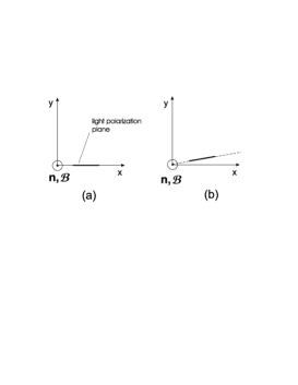
Figure 1: (a) Linearly polarized light with $\zeta_{3}=1$, $\zeta_{1}=\zeta_{2}=0$, (b) the light with $\zeta_{3}\approx 1$, $\zeta_{1}\neq 0$, $\zeta_{2}=0$.

Let us recall that $\zeta_{3}=1$ and $\zeta_{3}=-1$ corresponds to the light polarized along $x$ and $y$ axis respectively. The parameter $\zeta_{1}=\pm 1$ describes polarization at $45^{0}$ to the $y$ axis. The light ellipticity $\Psi$ is expressed through $\zeta_{2}=2\Psi$ for fully polarized light. Partially polarized light can be expanded as sum of natural light and elliptically polarized light. In this case $\zeta_{2}=2\Psi\,P$, where $P$ is light polarization and $\Psi$ is the ellipticity of the polarized part.

In the BMV project bmv it is planed to achieve an accuracy sufficient for the measurements of the vacuum birefringence predicted by QED, i.e., $\Delta n\sim 10^{-21}$ at ${\mathcal{B}}\sim 25~{}~{}\mbox{T}$. Earlier, $\Delta n\sim 1.3\times 10^{-20}$ was measured in the BNL experiment camer and $\Delta n\sim 6.7\times 10^{-20}$ by PVLAS pvlas . Thus, from measurements of $\Delta n$ corresponding to Faraday rotation at the level $\Delta n_{CPTL}=D\sim 10^{-21}$ in a magnetic field of 25 T (we’ll use the system of units $e^{2}/4\pi=\alpha,1\,\mbox{T}=195\,\mbox{eV}^{2},1\,\mbox{V}/\mbox{m}=6.5\times 10^{-7}\,\mbox{eV}^{2}$) one will be able to obtain the restriction $d_{1}=\frac{2D}{\mathcal{B}}\sim 4\times 10^{-13}~{}\mbox{MeV}^{-2}$.

The presence of a residual pressure in the resonator imposes restriction on the measurement of $\Delta n$ of the vacuum. Assuming the residual pressure in the equipment to be $10^{-11}$ Torr, we find that $\Delta n$ of the Faraday effect for helium at this pressure is $\Delta n\sim 10^{-22}$. Thus, CPT-violating Faraday effect can be measured with this accuracy.

For measurement of the terms, proportional to $b_{1}$ we may choose a magnetic field perpendicular to the photon wave vector. The electric field should be chosen perpendicular to both the photon wave vector and the magnetic field strength vector. Thus the photon wave vector, the direction of the magnetic field, and the direction of the electric field form triplet of mutually orthogonal vectors as shown in Fig. 2 and 3. The refractive index contains terms which are of odd or even order in the vector $\bm{n}$. For the laser experiment only the terms of even order in the wave vector are of interest, because these effects accumulate under the passage of a photon back and forth between the resonator mirrors footnote2 . Considering only these terms we find that all the coefficients $A=\frac{a_{1}}{2}({\mathcal{E}}^{2}+{\mathcal{B}}^{2})$, $B=2a_{2}({\mathcal{E}}^{2}+{\mathcal{B}}^{2})$, $C=-c_{1}{\mathcal{E}}{\mathcal{B}}$ and $D=-b_{1}{\mathcal{E}}{\mathcal{B}}+d_{3}/2$ are different from zero. First, assume that all the coefficients are approximately of the same order of magnitude. Then the light with the initial polarization $\zeta_{3}$ receives polarization $\zeta_{1}$. The polarization $\zeta_{1}$ can also arise due to imaginary part of the coefficient $C$, however, this contribution does not depend on the sign of the initial polarization $\zeta_{3}$ and can be separated by changing the sign of $\zeta_{3}$ during the experiment. Taking the electric field strength $\mathcal{E}\sim 10^{6}$ V/m we obtain a restriction on CPT and the causality violation constant $b_{1}=\frac{\Delta n^{\prime}_{CPT}}{\mathcal{E}\mathcal{B}}=\frac{D}{\mathcal{E}\mathcal{B}}\sim 0.31\,\mbox{MeV}^{-4}$ if $\Delta n^{\prime}_{CPT}$ is measured with accuracy $10^{-21}$. To measure CP-violating constant $c_{1}$ we have to search for the ellipticity parameter $\zeta_{2}$ when the light was initially linearly polarized with the $\zeta_{3}=1$.

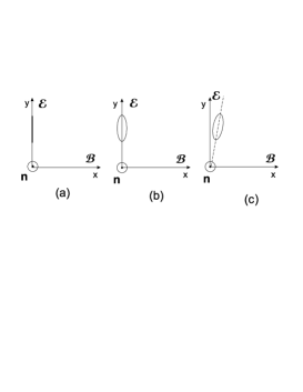
Figure 2: (a) Linearly polarized light with $\zeta_{3}=-1$, $\zeta_{1}=\zeta_{2}=0$, (b) the light with $\zeta_{3}\approx-1$, $\zeta_{2}\neq 0$ and $\zeta_{1}=0$, (c) the light with $\zeta_{3}\approx-1$, $\zeta_{2}\neq 0$ and $\zeta_{1}\neq 0$ (ellipse of polarization is slightly rotated).

In the case, when $\mid A-B\mid\gg\mid D\mid,\mid C\mid$ (but $\mid(A^{\prime}-B^{\prime})\omega z\mid\ll 1$) ”mixing” of the polarizations $\zeta_{1}$ and $\zeta_{2}$ occurs. Still, the light initially polarized with $\zeta_{3}$ will gain polarization $\zeta_{1}$ and $\zeta_{2}$ only in the case, when $C$ or $D$ differs from zero. But we will not know $C$ or $D$. Fortunately, we have a possibility to avoid this difficulty. The sign of the Cotton-Mouton effect for nitrogen is opposite to the sign of the vacuum Cotton-Mouton effect; therefore, using nitrogen at a residual pressure about $10^{-7}$ Torr we can compensate for the difference $A^{\prime}-B^{\prime}$ and distinguish $D$ from $C$.

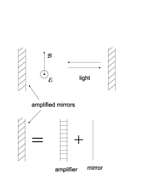
Figure 3: Scheme of a photon trap.

Apparently, the possibility exists to measure much smaller $\Delta n$. Baryshevsky offers an interesting idea of using laser amplifiers bar , which do not change polarization properties of light, but at the same time, will stop a photon beam damping. Ideally, the amplifier should be combined with a mirror, as shown in Fig. 3, to obtain ”amplified” mirror with the reflectivity 1 or more than 1. A light can be localized in such a trap for several hours. Assuming, for example, that we can measure an angle of polarization rotation $\Delta\theta=\Delta n\omega z\sim 10^{-10}$ and the lifetime of a photon in the trap is 1 hour, we’ll find the minimum measured $\Delta n\sim 10^{-27}$, for the $\omega=2.4~{}eV$. However a number of technical problems can arise in this scheme. For instance, we need the amplifier remaining isotropic after multiple passage of the polarized light through it.

Finally it may be possible to obtain restrictions on this CPT violating term examining the polarization of light, from the distant galaxies. It is necessary to separate the vacuum effects from the Faraday rotation in magnetic field and substance of galaxies. Earlier, such an analysis yields the restriction $\Delta n_{CS}=d_{3}\sim 10^{-33}$ ($\omega=2.4~{}eV$) jackiw for the term $\varepsilon^{ij}\sim e^{ijm}n^{m}$ (Chern-Simon term).

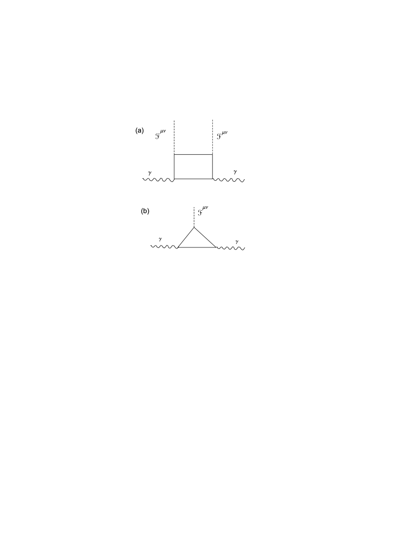
Figure 4: (a) QED graph of vacuum polarization contribution to the photon refractive index in a static field. (b) Analogous graph of C-odd vacuum polarization.

V Comparison of the laser experiment tests with some other known tests

Let us estimate CPT violation of the Faraday type $\sim e^{ijm}{\mathcal{B}}^{m}$. Certainly, we can not be sure of the applicability of the Feynman diagram technique in the case of CPT invariance violation. But it can still be suitable for heuristic estimates. In the framework of QED, the refractive index, proportional to $a_{1},a_{2}$, is evaluated using the square diagram shown in Fig. 4. Each vertex with the external electromagnetic field corresponds to the factor $\frac{e}{\sqrt{4\pi}}\frac{{\mathcal{B}}}{m^{2}}$ or $\frac{e}{\sqrt{4\pi}}\frac{{\mathcal{E}}}{m^{2}}$ in $\Delta n$, where $m$ is the electron mass. Each of the remaining vertices corresponds to the factor $e/\sqrt{4\pi}$. We can, in the same way, estimate CPT and Lorentz violating term $\sim e^{ijm}{\mathcal{B}}^{m}$, considering the triangle diagram shown in Fig. 4. The triangle diagram can not appear in standard QED, as the diagram is not invariant under C conjugation. Let us assume the most remarkable possibility, that the violation of C, CPT and Lorentz invariance is induced by some unknown particles interacting with the photons with C violation of the order of unity. By analogy with the calculation of the standard square diagram we assume that the vertex with the external field corresponds to the factor $\frac{g}{\sqrt{4\pi}}\frac{{\mathcal{B}}}{\mu^{2}}$ in $\Delta n$ and the others vertexes correspond to the factor $g/\sqrt{4\pi}$ in $\Delta n$, where $g$ is the coupling of the particle with photons and $\mu$ is the particle mass. As a result, we have

$$\Delta n_{CPTL}\approx\frac{{g}^{2}}{4\pi}\,\frac{{g}{\mathcal{B}}}{\sqrt{4\pi}\mu^{2}}.$$ (32)

In the BMV project it is planed to reach an accuracy sufficient for a measurement of $\Delta n$ predicted by QED, i.e., $\Delta n\sim 10^{-21}$ (strength of the magnetic field is 25 T ) A measurement of $\Delta n_{CPTL}$ with such an accuracy gives a restriction on the coupling $g$. It is interesting to compare this restriction with what follows from the CPT test, based on a comparison of the g factors of an electron and positron: $\alpha_{CPT}=\frac{\mbox{g}_{e^{+}}-\mbox{g}_{e^{-}}}{\mbox{g}_{avr}}<10^{-12}$ part . Under the assumption of the same mechanism of C parity violation, $\alpha_{CPT}$ arises from the diagram shown in Fig. 5(b).

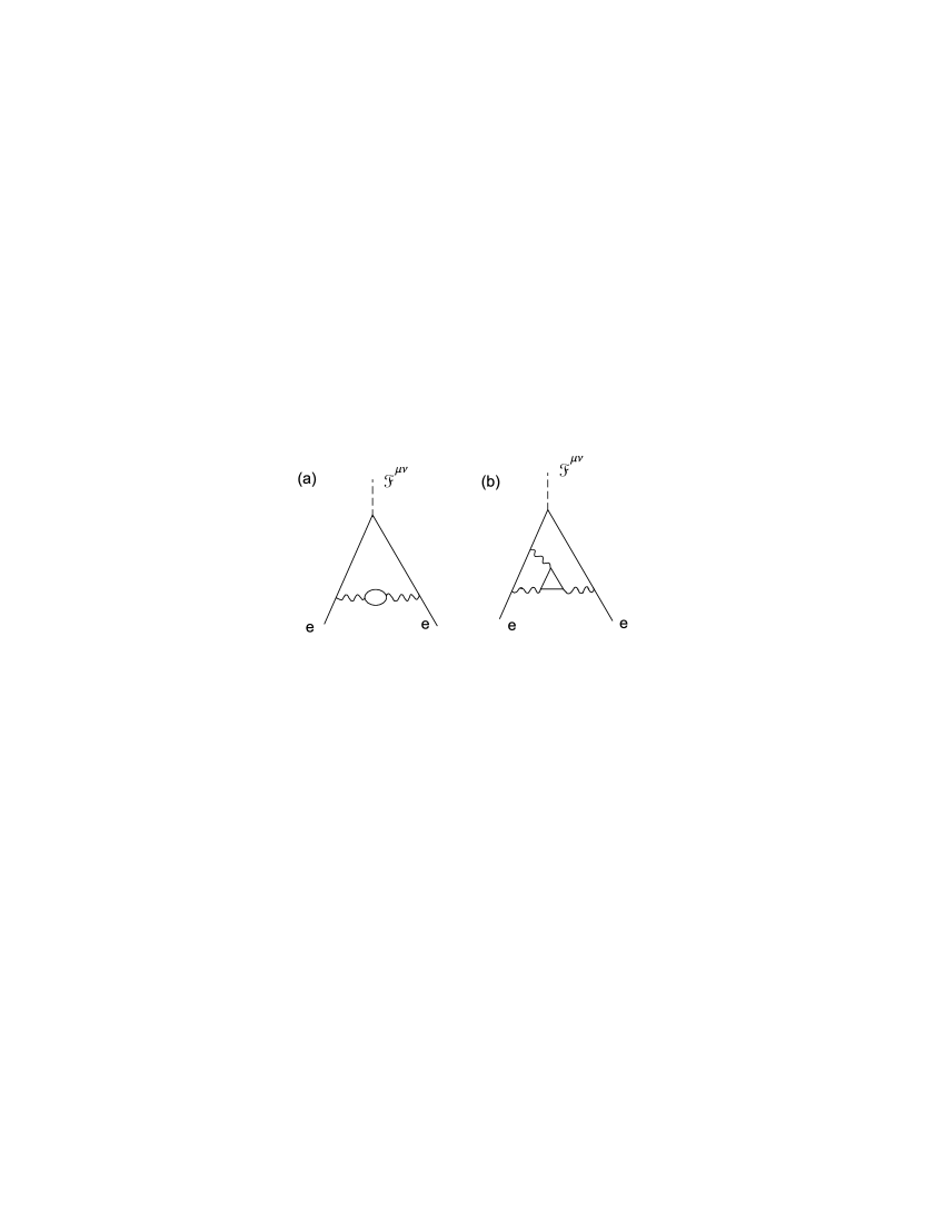
Figure 5: (a) Graph of vacuum polarization contribution to the electron or positron g-factor. (b) Analogous graph of C-odd vacuum polarization.

For the sake of simplicity, we again make very heuristic estimates of the diagram shown in Fig. 5(b). First, we remark that the relative contribution of the diagram shown in Fig. 5(a) (usual vacuum polarization) to the g-factor of the electron is $\sim\frac{e^{4}}{(4\pi)^{2}}\frac{m^{2}}{\mu^{2}}$ if a virtual particle mass $\mu\gg m$, and is $\sim\frac{e^{4}}{(4\pi)^{2}}\ln{\frac{m}{\mu}}$ when $\mu\ll m$ lan4 . This fact is a reflection of a more general rule. The contribution of the virtual particle loop connected by the photon lines to the electrons is proportional to some degrees of $\frac{m}{\mu}$ when $\mu\gg m$, and to some degrees of $\ln{\frac{m}{\mu}}$ when $\mu\ll m$. Thus, the contribution of the diagram shown in Fig. 5(b) can be estimated as

$$\alpha_{CPT}\approx\frac{e^{3}{g}^{3}}{(4\pi)^{3}}F\left(\frac{m^{3}}{\mu^{3}}\right),$$ (33)

where the Spens function $F(x)$ lan4 has the asymptotic $F(x)\approx x$ when $x\ll 1$ and $F(x)\approx\frac{\pi^{2}}{6}+\frac{1}{2}\ln^{2}(x)$ when $x\gg 1$.

Figure 6: Restrictions on the dimensionless coupling $g$ of some particles interacting with photons, with the relative C, CP, CPT and Lorentz invariance violation of order unity. The straight curve relates the Faraday effect in vacuum and corresponds to the inequality $\Delta n_{CPTL}<10^{-21}$. The bent curve arises from the difference of electron and positron g-factors and corresponds to the inequality $\frac{\mbox{g}_{e^{+}}-\mbox{g}_{e^{-}}}{\mbox{g}_{avr}}<10^{-12}$.

Fig. 6 shows restrictions on the coupling $g$ of C-, CP -, CPT- and Lorentz-violating interaction following from the inequalities $\Delta n_{CPTL}<10^{-21}$ and $\alpha_{CPT}<10^{-12}$. As we can see, measurement of the Faraday effect in vacuum gives much more stringent restrictions on $g$ in the above model of CPT violation than the traditional comparison of the electron and positron g-factors. Certainly, it happens because we have chosen the model with CPT violation in the photon sector; therefore, the experiments dealing directly with photons have an advantage.

Let us now consider the terms proportional to $b_{1}$, which breaks P , CP , CPT and causality, but at the same time, are Lorentz invariant and do not break C-parity. To estimate of the appropriate $\Delta n_{CPT}^{\prime}$ we should consider the square diagram of Fig. 4(a). In the same way we find:

$$\Delta n_{CPT}^{\prime}\sim\frac{{g}^{\prime 2}}{4\pi}\,\left(\frac{{g}^{\prime}{\mathcal{B}}}{\sqrt{4\pi}\mu^{2}}\right)\left(\frac{{g}^{\prime}{\mathcal{E}}}{\sqrt{4\pi}\mu^{2}}\right).$$ (34)

The restriction on ${g}^{\prime}$, obtained from a measurement of $\Delta n_{CPT}^{\prime}$ with the accuracy $10^{-21}$, can be compared, for example, with the restriction on CP violation in para-positronium decay in two photons. Positronium ${}^{1}S_{0}$ state has negative spatial parity lan4 ; therefore, the probability of decay into two polarized photons should be proportional to $(\bm{e}_{1}\times\bm{e}_{2}\cdot\bm{k})$ perk , where $\bm{e}_{1}$ and $\bm{e}_{2}$ are the photon polarizations, $\bm{k}$ is the momentum of one of the photons (another photon has opposite momentum). The presence of the P-even $(\bm{e}_{1}\cdot\bm{e}_{2})$ correlation is a signal of P and CP violation (C parity conserves in para-positronium two photon decay). For this process we can say nothing about T invariance, because we do not compare it with the reverse process of the $\gamma+\gamma\rightarrow Ps$.

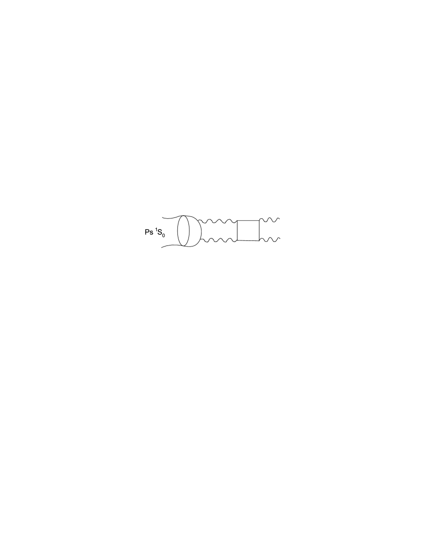
Figure 7: Graph of P-violating photon interaction in final state in the two photon para-positronium decay.

The branching ratio $\alpha_{CP}^{\prime}$ of the decay with the $(\bm{e}_{1}\cdot\bm{e}_{2})$ can be estimated from the diagram shown in Fig. 7 and is given by

$$\alpha_{CP}^{\prime}\sim\frac{g^{\prime 4}}{(4\pi)^{2}}F\left(\frac{m^{4}}{\mu^{4}}\right).$$ (35)

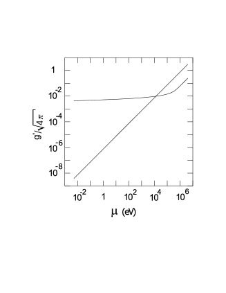
Figure 8: Restrictions on the dimensionless coupling $g^{\prime}$ of the particles interacting with photons with violation of parity, CP, CPT and causality of an order unity, but conserving Lorentz invariance. The restrictions follow from the inequality $\Delta n_{CPT}^{\prime}<10^{-21}$ (straight curve) and the inequality $\alpha_{CP}^{\prime}<10^{-6}$ (bent curve).

The restrictions on ${g}^{\prime}$, following from the inequality $\Delta n_{CPT}^{\prime}<10^{-21}$ and $\alpha_{CP}^{\prime}<10^{-6}$ are shown in Fig.8. We have taken the electric field strength $10^{6}$ V/m, so that the dimensionless parameter $\left(\frac{e{\mathcal{E}}}{m^{2}}\right)\sim 10^{-12}$. The vertexes, we have considered, are of the type one photon — two particles, however, it is possible to consider a vertex of the type two photons — one particle. In this case for evaluation of $\Delta n_{CPT}^{\prime\prime}$ we should to consider the diagram shown in Fig. 9. From the reasons of dimensionality we obtain:

$$\Delta n_{CPT}^{\prime\prime}\sim\left(\frac{{g}^{\prime\prime}{\mathcal{B}}}{\sqrt{4\pi}\mu^{2}}\right)\left(\frac{{g}^{\prime\prime}{\mathcal{E}}}{\sqrt{4\pi}\mu^{2}}\right).$$ (36)

Figure 9: CPT violation due to exchange of causality violating particle (tachyon) of axion type.

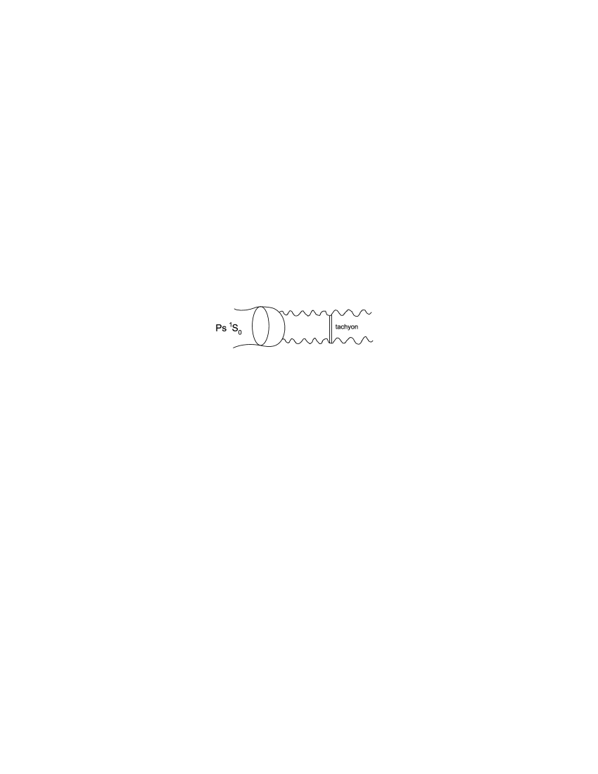
Figure 10: Tachyon induced CP violation in the two-photon decay of para-positronium.

CP violation in positronium decay can be estimated from the diagram shown in Fig. 10 as

$$\alpha_{CP}^{\prime\prime}\sim\frac{{g}^{\prime\prime 2}}{4\pi}F\left(\frac{m^{2}}{\mu^{2}}\right).$$ (37)

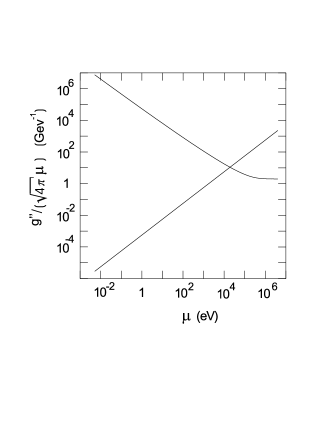
Figure 11: Restrictions on the tachyon coupling arising from the inequality $\Delta n^{\prime\prime}_{CPT}<10^{-21}$ (straight curve) and from the inequality $\alpha_{CP}^{\prime\prime}<10^{-6}$ (bent curve).

Unfortunately, due to the weakness of the electric field possible in a laser experiment, compared to the magnetic one, restriction on a such CPT and causality breaking tachyon coupling are $\sqrt{\frac{\mathcal{E}}{\mathcal{B}}}$ times weaker than the restriction on the usual axion coupling for which $\Delta n\sim\left(\frac{{g}_{a}{\mathcal{B}}}{\sqrt{4\pi}\mu^{2}}\right)^{2}$. For the strength of the electric and magnetic fields, used in our work, this gives about 100 times difference. For the usual axion the very rigid restriction $\frac{g_{a}}{\sqrt{4\pi}\mu_{a}}\sim 10^{-9}-10^{-10}~{}~{}\mbox{Gev}^{-1}$ follow from astrophysics raf . However, laser experiments can be considered irrespective of the models as independent tests of CPT invariance.

VI Conclusion

To summarize, laser experiments on searching CPT, Lorentz invariance and causality violation for photons in vacuum, in the presence of constant uniform magnetic and electrical fields, are competitive with tests using positron and electron g-factors comparison and searching of CP violation in positronium decay, provided, that CPT is broken in the photon sector. It is essential, that in the case of unbroken Lorentz invariance we have the possibility of testing causality and locality.

APPENDIX A

In this appendix we consider the structure of the tensor ${\mathcal{P}}^{\mu\nu}$ in the external field, including of mass shell terms. Despite the above classical consideration the expansion of the tensor ${\mathcal{P}}^{\mu\nu}$ in the orders of ${\mathcal{F}}^{\mu\nu}$ and $k^{\mu}$ is not only valid for soft photons. In fact we can deduce it by considering one-photon retarded Green’s function in the external stationary uniform electromagnetic field ${\mathcal{D}}_{\mu\nu}(x-x^{\prime})=i<0\mid[\hat{A}_{\mu}(x),\hat{A}_{\nu}(x^{\prime})]\mid 0>\theta(t-t^{\prime})$. The photon propagation modes can be described by the poles of the Fourier transform ${\mathcal{D}}_{\mu\nu}(k)=\int{\mathcal{D}}_{\mu\nu}(x)e^{ikx}d^{4}x$ of the Green’s function. The dispersion relation for the propagation modes reads

$$det\mid{\mathcal{D}^{-1}_{\mu\nu}(k)}\mid=0.$$ (38)

The photon Green’s function is expressed through the Green’s function of the free photon $D_{\mu\nu}(k)$ and the polarization operator as

$${\mathcal{D}}_{\mu\nu}(k)=D_{\mu\nu}(k)+D_{\mu\alpha}(k){\mathcal{P}}^{\alpha\beta}(k){\mathcal{D}}_{\beta\nu}(k).$$

Thus ${\mathcal{D}}_{\mu\nu}^{-1}=D_{\mu\nu}^{-1}-{\mathcal{P}}^{\mu\nu}.$ Taking $D_{\mu\nu}^{-1}(k)=\left(k^{2}g_{\mu\nu}-k_{\nu}k_{\mu}\right)$ we come to a dispersion relation congruous to Eqs.(2) and (3).

Tensor 4x4 ${\mathcal{P}}^{\mu\nu}$ contains 16 independent components. Thus it can be expanded over 16 independent tensors. Ten of them are symmetric and 6 are antisymmetric. The gauge invariance condition ${\mathcal{P}}^{\mu\nu}k_{\nu},~{}~{}\mu\{0,1,2,3\}$ reduces the number of symmetric terms to 6. It also reduces the number of antisymmetric terms to 3, because for any antisymmetric tensor $k_{\mu}{\mathcal{P}}^{\mu\nu}k_{\nu}=0$ is automatically valid and only three of four gauge conditions are independent. Independent tensors should be expressed through the tensor of an external field ${\mathcal{F}}^{\mu\nu}$ and the photon wave vector $k$. The expansion can be written as

$${\mathcal{P}}^{\mu\nu}=a_{0}(k^{2}g^{\mu\nu}-k^{\mu}k^{\nu})+a_{1}{\mathcal{F}}^{\mu\alpha}k_{\alpha}{\mathcal{F}}^{\nu\sigma}k_{\sigma}+4a_{2}\tilde{\mathcal{F}}^{\mu\alpha}k_{\alpha}\tilde{\mathcal{F}}^{\nu\sigma}k_{\sigma}+2c_{1}(\tilde{\mathcal{F}}^{\mu\alpha}k_{\alpha}{\mathcal{F}}^{\nu\sigma}k_{\sigma}+{\mathcal{F}}^{\mu\alpha}k_{\alpha}\tilde{\mathcal{F}}^{\nu\sigma}k_{\sigma})$$

$$+c_{2}[(k^{2}{\mathcal{F}}^{\mu\alpha}{\mathcal{F}}_{\alpha\lambda}k^{\lambda}-k^{\mu}k^{\delta}{\mathcal{F}}_{\delta\beta}{\mathcal{F}}^{\beta\sigma}k_{\sigma}){\mathcal{F}}^{\nu\rho}k_{\rho}+(k^{2}{\mathcal{F}}^{\nu\alpha}{\mathcal{F}}_{\alpha\lambda}k^{\lambda}-k^{\mu}k^{\delta}{\mathcal{F}}_{\delta\beta}{\mathcal{F}}^{\beta\sigma}k_{\sigma}){\mathcal{F}}^{\mu\rho}k_{\rho}]$$

$$+c_{3}[(k^{2}{\mathcal{F}}^{\mu\alpha}{\mathcal{F}}_{\alpha\lambda}k^{\lambda}-k^{\mu}k^{\delta}{\mathcal{F}}_{\delta\beta}{\mathcal{F}}^{\beta\sigma}k_{\sigma})\tilde{\mathcal{F}}^{\nu\rho}k_{\rho}+(k^{2}{\mathcal{F}}^{\nu\alpha}{\mathcal{F}}_{\alpha\lambda}k^{\lambda}-k^{\mu}k^{\delta}{\mathcal{F}}_{\delta\beta}{\mathcal{F}}^{\beta\sigma}k_{\sigma})\tilde{\mathcal{F}}^{\mu\rho}k_{\rho}]$$

$$+b_{1}\,e^{\mu\nu\alpha\beta}k_{\alpha}{\mathcal{F}}_{\beta\eta}{\mathcal{F}}^{\eta\phi}k_{\phi}+b_{2}\,e^{\mu\nu\lambda\alpha}{\mathcal{F}}_{\lambda\sigma}k^{\sigma}k_{\alpha}+b_{3}\,(k^{\mu}{\mathcal{F}}^{\nu\lambda}k_{\lambda}-k^{\nu}{\mathcal{F}}^{\mu\lambda}k_{\lambda}+k^{2}{\mathcal{F}}^{\mu\nu}),$$ (39)

where $\tilde{\mathcal{F}}^{\mu\nu}=\frac{1}{2}e^{\mu\nu\eta\delta}{\mathcal{F}}_{\eta\delta}$. Coefficients $a_{0},a_{1},\dots$ are functions of four independent scalars $k^{2}$, $k_{\mu}{\mathcal{F}}^{\mu\nu}{\mathcal{F}}_{\nu\lambda}k^{\lambda}$, $\Im={\mathcal{F}}_{\mu\nu}{\mathcal{F}}^{\mu\nu}$, ${\mathcal{G}}={\mathcal{F}}_{\mu\nu}\tilde{\mathcal{F}}^{\mu\nu}$ shabad . The terms involving $a_{0},c_{2},c_{3},b_{2},b_{3}$ do not lead to observable effects at first order in the constants, because evaluation of these terms on the photon mass shell gives zero. For instance, the quantity $e^{*\mu}(k^{2}g_{\mu\nu}-k_{\mu}k_{\nu})e^{\nu}$ equals to zero because the free photon satisfies $k^{2}=0$ and $ek=0$. The symmetry properties of the all the terms are given in the table. Let us remark that the scalar $\mathcal{G}$ is P- and T- violating so if the coefficients $a_{0},a_{1}\dots$ contain odd orders of $\mathcal{G}$ its symmetry properties change. Conventional QED allows the terms proportional to $a_{0},a_{1},a_{2}$ and also the term involving $c_{1}$ which appears only with the odd degree of ${\mathcal{G}}$. In a pure magnetic field ${\mathcal{G}}=0$ and the aforementioned term disappears.

Table 1: Symmetry properties of the terms of tensor ${\mathcal{P}}^{\mu\nu}$ allowed by Lorentz and gauge invariance.

	Symmetry		Observability
Term	Base	Modified by ${\mathcal{G}}^{2n+1}$	with real
	C P T	C P T	photons
$a_{0}$	$+$ $+$ $+$	$+$ $-$ $-$	invisible
$a_{1}$	$+$ $+$ $+$	$+$ $-$ $-$	visible
$a_{2}$	$+$ $+$ $+$	$+$ $-$ $-$	$<>$
$c_{1}$	$+$ $-$ $-$	$+$ $+$ $+$	$<>$
$c_{2}$	$-$ $+$ $-$	$-$ $-$ $+$	invisible
$c_{3}$	$-$ $-$ $+$	$-$ $+$ $-$	$<>$
$b_{1}$	$+$ $-$ $+$	$+$ $+$ $-$	visible
$b_{2}$	$-$ $+$ $+$	$-$ $-$ $-$	invisible
$b_{3}$	$-$ $-$ $-$	$-$ $+$ $+$	$<>$

APPENDIX B

Here we deduce Eq.(8) from the field-theoretic Schroedinger equation. The classical 4-current $j_{\mu}(\bm{r},t)$ corresponds to some Schroedinger operator $\hat{j}_{\mu}(\bm{r})$, so that perturbation of the vacuum in a constant fields by the electromagnetic wave can be described by the interaction Hamiltonian $\hat{V}(t)=\int\hat{j}^{\mu}(\bm{r})A_{\mu}(x)d^{3}r$. Let’s recall that $A(x)$ represents the 4-potential of the wave. We’ll assume that the wave rise adiabatically from zero value at infinity. A perturbed state of the system is described by the Schroedinger equation.

$$\frac{d}{dt}\mid t>=(\hat{H}_{0}+\hat{V})\mid t>.$$ (40)

Vacuum states in the constant external fields are eigenstates of the Hamiltonian $\hat{H}_{0}$ in the absence of wave: $\hat{H}_{0}\mid n>=\varepsilon_{n}\mid n>$. Expansion of the state $\mid t>$ to states $\mid n>$ gives

$$\mid t>=\mid 0>+\sum_{n\neq 0}a_{n}(t)|n>e^{-i\varepsilon_{n}t}.$$ (41)

Substituting the given expression to Eq. (40) we obtain:

$$i\frac{da_{n}(t)}{dt}=<n|\hat{V}(t)|0>e^{i\varepsilon_{n}t}.$$ (42)

Using the Fourier transform of the wave 4-potential $A_{\mu}(x)=\int A_{\mu}(k)e^{-ikx}d^{4}x$ and the translational invariance of vacuum $<n|\hat{j}_{\mu}(\bm{r})|0>=<n|\hat{j}_{\mu}(0)|0>e^{-i\bm{p}_{n}\bm{r}}$ we obtain

$$<n|\hat{V}(t)|0>=\int<n|\hat{j}^{\mu}(\bm{r})|0>e^{i\varepsilon_{n}t-ikx}A_{\mu}(k)d^{4}kd^{3}\bm{r}=\int<n|\hat{j}^{\mu}(0)|0>e^{ip_{n}x-ikx}A_{\mu}(k)d^{4}kd^{3}\bm{r}$$

$$=(2\pi)^{3}<n|\hat{j}^{\mu}(0)|0>\int\delta^{(3)}(\bm{p}_{n}-\bm{k})e^{i\varepsilon_{n}t-i\omega t}A_{\mu}(k)d^{4}k.$$ (43)

The solution of Eq. (42) can be written as

$$a_{n}(t)=-i\int^{t}_{-\infty}<n|\hat{V}(\tau)|0>e^{i\varepsilon_{n}\tau}d\tau=(2\pi)^{3}<n|\hat{j}^{\mu}(0)|0>\int\delta^{(3)}(\bm{p}_{n}+\bm{k})\frac{e^{i\varepsilon_{n}t-i\omega t}}{\omega-\varepsilon_{n}+i0}A_{\mu}(k)d^{4}k.$$ (44)

Then we can find the average value of $\hat{j}(\bm{r})$. Evaluation of $j(\bm{r},t)=<t\mid\hat{j}(\bm{r})\mid t>$ with the help of $a_{n}(t)$ given by Eq. (44) leads to

$$j_{\mu}(x)=-(2\pi)^{3}\int\sum_{n\neq 0}\biggl{(}<n|\hat{j}^{\nu}(0)|0>\delta^{(3)}(\bm{p}_{n}-\bm{k})\frac{e^{i(\varepsilon_{n}-\omega)t}}{\varepsilon_{n}-\omega-i0}A_{\nu}(k)<0|\hat{j}_{\mu}(x)|n>$$

$$+<0|\hat{j}^{\nu}(0)|n>\delta^{(3)}(\bm{p}_{n}-\bm{k})\frac{e^{-i(\varepsilon_{n}-\omega)t}}{\varepsilon_{n}-\omega+i0}A^{*}_{\nu}(k)<n|\hat{j}_{\mu}(x)|0>\biggr{)}d^{4}k$$

$$=-(2\pi)^{3}\int\sum_{n}\biggl{(}<0|\hat{j}_{\mu}(0)|n><n|\hat{j}^{\nu}(0)|0>\frac{\delta^{(3)}(\bm{p}_{n}-\bm{k})}{\varepsilon_{n}-\omega-i0}$$

$$+<0|\hat{j}^{\nu}(0)|n><n|\hat{j}_{\mu}(0)|0>\frac{\delta^{(3)}(\bm{p}_{n}+\bm{k})}{\varepsilon_{n}+\omega+i0}\biggr{)}A_{\nu}(k)e^{-ikx}d^{4}k.$$ (45)

From Eq. (45), in view of the definition given by Eq. (3) we obtain Eq. (12), which is the Fourier transform of Eq. (8). Let’s note, that the Fourier transform of the causal polarization operator

$$\Pi_{\mu\nu}(x)=4\pi i<0|T\hat{j}_{\mu}(x)\hat{j}_{\nu}(0)|0>$$ (46)

differs from (12) by the sign before $i0$ in the second term. For the photon refractive index it is necessary to use just the delayed polarization operator ${\mathcal{P}}_{\mu\nu}$, as in this case ${\mathcal{P}}^{\mu\nu}(k)$ given by Eq. (12) has the right properties ${\mathcal{P}}^{*}_{\mu\nu}(k)={\mathcal{P}}_{\mu\nu}(-k)$ required by a reality of the field $A(x)$.

References

• (1) R. Cameron et al., Phys. Rev. D 47, 3707 (1993).
• (2) E. Zavattini et al. in Quantum Electrodynamics and Physics of the Vacuum, proceedings of International Workshop, Trieste, Italy, 2000, edited by G. Cantatore, (AIP, Melville-New-York, 2001), p. 77.
• (3) S. Askenazy et al. in Quantum Electrodynamics and Physics of the Vacuum, proceedings of International Workshop, Trieste, Italy, 2000, edited by G. Cantatore, (AIP, Melville-New-York, 2001), p. 115.
• (4) J. H. Christenson, J.W. Cronin, V.L. Fitch, and R. Turlay, Phys.Rev.Lett. 13, 138 (1964).
• (5) K. Abe et al., Phys.Rev.Lett. 87, 091802 (2001).
• (6) A. Angelopoulos et al., Phys.Lett. 444B, 43 (1998).
• (7) J. Schwinger, Phys.Rev. 82, 664 (1951);D.M. Gitman, E.S. Fradkin, and Sh. M. Shvartsman, Tr.Fiz.Inst.Akad.Nauk SSSR 193, 3 (1989).
• (8) I.A. Batalin and A.E. Shabad, Zh.Eksp.Teor.Fiz. 60, 894 (1971)[Sov.Phys.β€”JETP, 33, 483 (1971)];A.E. Shabad, Ann.Phys.(NY) 90, 166 (1975); Tr.Fiz.Inst.Akad.Nauk SSSR 192, 5 (1988).
• (9) Transversity of ${\mathcal{P}}^{\mu\nu}$ following from current conservation strongly restricts the ${\mathcal{P}}^{\mu\nu}$ structure, forbidding, for example, the terms ${\mathcal{P}}^{\mu\nu}\sim{\mathcal{F}}^{\mu\nu}$ and ${\mathcal{P}}^{\mu\nu}\sim e^{\mu\nu\delta\eta}{\mathcal{F}}_{\delta\eta}$, which could lead to the three dimensional terms $\varepsilon^{ij}\sim e^{ijm}{\mathcal{B}}^{m}$ and $\varepsilon^{ij}\sim e^{ijm}{\mathcal{E}}^{m}$ in the dielectric constant. For massless photons current conservation arises automatically when we multiply Eq. (2) by $k^{\mu}$. Some models suggest existence of massive photons, violating gauge invariance. This can be described by the introduction of an effective ”mass term” ${\mathfrak{m}}^{2}A^{\mu}(k)$ into Eq. (2). Current conservation no longer arises automatically. Still we may demand it together with the Lorentz gauge $k_{\mu}A^{\mu}(k)=0$. For theories that do not suggest this, gauge nontransversal part of ${\mathcal{P}}^{\mu\nu}$ can be estimated by multiplying Eq. (2) with mass term by $k_{\mu}$. We find that the nontransversal part of ${\mathcal{P}}^{\mu\nu}\sim{\mathfrak{m}}^{2}$. From Eq. (4) we find the corresponding part of the refractive index $\Delta n\sim\frac{{\mathfrak{m}}^{2}}{\omega^{2}}$. Geomagnetic data lead to the limit ${\mathfrak{m}}<3\times 10^{-24}$ GeV geo , while observations of the galactic magnetic field give ${\mathfrak{m}}<3\times 10^{-36}$ GeV magn ; thus $\Delta n\sim 10^{-30}-10^{-54}$ for $\omega\sim 3$ eV. Therefore the transversity of ${\mathcal{P}}^{\mu\nu}$ that we have used is justified in any case.
• (10) A. Goldhaber and M. Nieto, Rev. Mod. Phys. 43, 277 (1971).
• (11) G. Chibisov, Usp. Fiz. Nauk 119, 551 (1976) [Sov. Phys. Usp. 19, 624 (1976)].
• (12) R.F. Streater and A.S. Wightman, PCT, spin and statistics and all that (W.A. Benjamin, Inc., New-York-Amsterdam, 1964).
• (13) D. Colladay and V.A. KosteleckΓ½, Phys. Rev. D 55, 6760 (1997); 58, 116002 (1998); V.A. KosteleckΓ½ and R. Lehnert, Phys. Rev. D 63, 065008 (2001).
• (14) S.L. Adler, Ann.Phys.(NY) 67, 599 (1971); Z. Bialynicka-Birula and I. Bialynicka-Birula, Phys.Rev. D 2, 2341 (1970).
• (15) V.B. Berestetskii, E.M. Lifshitz, and L.P. Pitaevskii, Quantum electrodynamics (Pergamon Press, Oxford, 1982).
• (16) Nonrelativistic tensor structure of the dielectric constant in a substance was considered by N.B. Baranova, Yu.V. Bogdanov and B.Ya Zel’dovich, Usp. Fiz. Nauk 123, 349 (1977) [Sov. Phys. Usp. 20, 870 (1977)].
• (17) G.V. Efimov and Kh. Namsrai, Teor. & Mat. Fiz. 50, 221 (1982) [Teor. & Math. Phys. 50, 144 (1982)].
• (18) V.P. Barashev, A.E. Shabad and Sh. M. Shvartsman, Yad. Fiz. 43, 964 (1986) [Sov. J. Nucl. Phys. 43, 617 (1986)].
• (19) R. Krajcik and M. Nieto, Phys. Rev. 13, 924 (1976); 15, 445 (1977).
• (20) M.M. Gorshkov, Ellipsometry (Sov. Radio, Moscow, 1974).
• (21) Use of a $\lambda/4$ plate before a mirror allows to accumulate terms containing odd number of $\bm{n}$. This scheme could have a great advantage in measuring $b_{1}$ because an electric field is no longer needed. Still we do not discuss the scheme here as it was suggested long ago hrip but was not implemented yet, probably due to uncontrolled systematic errors.
• (22) I.B. Khriplovich, Parity nonconcervation in atomic phenomena(Gordon & Breach, London, 1991).
• (23) V. Baryshevsky, in Actual Problems of Particle Physics, proceedings of International School-Seminar, Gomel, Belarus, 1999, edited by A. Bogush et al., (JINR, Dubna, 2000), Vol. II, p.93; hep-ph/0007353.
• (24) G. Raffelt and L. Stodolsky, Phys. Rev. D 37, 1237 (1988).
• (25) S.M. Carroll, G.B. Field, and R. Jackiw, Phys. Rev. D 41, 1231 (1990); S.M. Carroll and G.B Field, Phys. Rev. Lett. 79, 2394 (1997).
• (26) Review of Particle Physics, Eur. Phys. J. C 15, 1 (2000).
• (27) D.H. Perkins, Introduction into High Energy Physics (Addison-Wesley, Inc., New-York, 1987).
• (28) G.G Raffelt, Phys. Rep. 198, 1 (1990).