Numerical evaluation of general massive 2-loop self-mass master integrals from differential equations

Abstract

The system of 4 differential equations in the external invariant satisfied by the 4 master integrals of the general massive 2-loop sunrise self-mass diagram is solved by the Runge-Kutta method in the complex plane. The method offers a reliable and robust approach to the direct and precise numerical evaluation of Feynman graph integrals.

The relevance of the higher order calculations for the comparison with nowadays precision measurements in high energy physics is well known and comprehensively presented by G. Passarino in this conference.

Therefore can be of some interest the exploitation of an alternative method (but still in the context of the integration by part identities and master integrals (MI) [1]) to the more common direct integration method for the numerical evaluation of the MI.

The method uses directly the differential equations. Starting from the integral representation of the MI, related to a certain Feynman graph, by derivation with respect to one of the internal masses [2] or one of the external invariants [3] and with the repeated use of the integration by part identities, a system of independent first order partial differential equations is obtained in a number equal to the number of the MI (master differential equations).

Enlarging the number of loops and legs grows the number of parameters, MI and equations, but does not change or spoil the method.

To solve the system of equations (analytically or numerically) it is necessary to know the MI for a chosen value of the differential parameter. To achieve that analytically comes out to be the most laborious part of the method and often requires some external knowledge, like the assumption of regularity of the solution in the value. Moreover, if the chosen value is a zero for one of the coefficients of the derivative of the MI in the equations (as is always the case in analytical calculations), also the first derivative for that value is necessary to work out the numerical solution for different values of the parameter, but this usually comes out to be a simpler task (unless poles in the limit of the number of dimensions $n$ going to 4 are present).

To test the method we have chosen the simple, but not trivial, 2-loop sunrise graph with arbitrary masses [4, 5], shown in Fig.1.

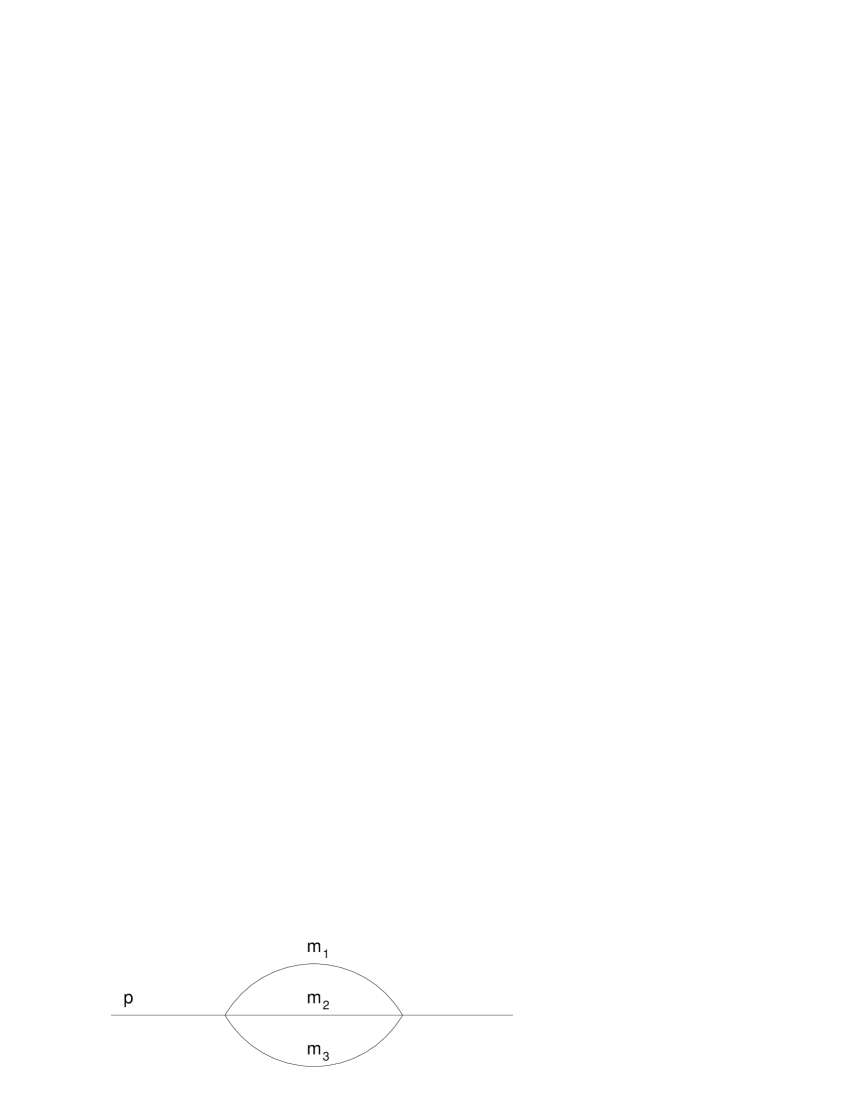
Figure 1: The general massive 2-loop sunrise self-mass diagram.

This graph is one of the topologies of the 2-loop self-mass and has 4 MI, the other topologies with 4 and 5 propagators have one more MI each [6, 7].

When the sunrise MI are expanded in $(n-4)$, the coefficients of the poles can be known analytically for arbitrary values of the external squared momentum $p^{2}$, while the finite parts satisfy the differential equations. From these equations the analytic expressions for their first order expansion were completed at the special points [4, 8, 9, 5]: $p^{2}=0$; $p^{2}=\infty$; $p^{2}=-(m_{1}+m_{2}+m_{3})^{2}$, the threshold; $p^{2}=-(m_{1}+m_{2}-m_{3})^{2}$, the pseudo-thresholds.

To obtain numerical results for arbitrary values of $p^{2}$, a 4th-order Runge-Kutta formula is implemented in a FORTRAN code, with a solution advancing path starting from the special points, so that also the first term in the expansion is necessary.

The path followed starts usually from $p^{2}=0$ and moves in the lower half complex plane of $p^{2}$ to avoid proximity to the other special points, which can cause loss in precision. For values of $p^{2}$ very close to a special point, we start from the analytical expansion at that special point. Remarkable self-consistency checks are provided by choosing different paths or different starting points to calculate the same value.

The execution of the program is rather fast and precise: with an Intel Pentium III of 1 GHz we get values with 7 digits requiring times ranging from a fraction of a second to 10 seconds of CPU, and with 11 digits from few tens of seconds to one hour.

If $\Delta=L/N$ is the length of one step, $L$ is the length of the whole path and $N$ the total number of steps, the 4th-order Runge-Kutta formula discards terms of order $\Delta^{5}$, so the whole error is $\epsilon_{RK}=N\Delta^{5}=L^{5}/N^{4}$, and a proper choice of $L$ and $N$ allows the control of the precision.

Indeed we estimate the relative error, as usual, by comparing a value obtained with $N$ steps with the one obtained with $N/10$ steps, $\epsilon_{RK}=[V(N)-V(N/10)]/V(N)$, to which we add a cumulative rounding error $\epsilon_{cre}=\sqrt{N}\times 10^{-15}$, due to our 15 digits double precision.

Comparisons are done in [5] with some values present in the literature [10, 11] with excellent agreement.

References

- [1] F.V. Tkachov, Phys. Lett.B 100, 65 (1981); K.G. Chetyrkin and F.V. Tkachov, Nucl. Phys.B 192, 159 (1981).
- [2] A.V. Kotikov, Phys. Lett.B254, 158 (1991).
- [3] E. Remiddi, Nuovo Cim.A110, 1435 (1997), hep-th/9711188.
- [4] M. Caffo, H. Czyż, S. Laporta and E. Remiddi, Nuovo Cim.A 111, 365 (1998), hep-th/9805118.
- [5] M. Caffo, H. Czyż and E. Remiddi, Nucl. Phys.B 634, 309 (2002), hep-ph/0203256.
- [6] O.V. Tarasov, Nucl. Phys.B 502, 455 (1997), hep-ph/9703319.
- [7] M. Caffo, H. Czyż, S. Laporta and E. Remiddi, Acta Phys. Pol.B 29, 2627 (1998), hep-th/9807119.
- [8] M. Caffo, H. Czyż and E. Remiddi, Nucl. Phys.B 581, 274 (2000), hep-ph/9912501.
- [9] M. Caffo, H. Czyż and E. Remiddi, Nucl. Phys.B 611, 503 (2001), hep-ph/0103014.
- [10] F.A. Berends, M. Böhm, M. Buza and R. Scharf, Z. Phys.C 63, 227 (1994).
- [11] G. Passarino, Nucl. Phys.B 619, 257 (2001), hep-ph/0108252.