Lepton Asymmetry in Polarized Drell-Yan

Abstract

The lepton helicity distributions in the polarized Drell-Yan process at RHIC energy are investigated. In the absence of the weak interaction, only the measurement of lepton helicity can prove the antisymmetric part of the hadronic tensor. Therefore it might be interesting to consider the helicity distributions of leptons to obtain more information on the structure of nucleon from the polarized Drell-Yan process. We estimate the QCD corrections at ${\cal O}(\alpha_{s})$ level to the hadronic tensor including both intermediate $\gamma$ and $Z$ bosons. We report the numerical analyses on the $Z$ pole and show that the $u(\bar{u})$ and $d(\bar{d})$ quarks give different and characteristic contributions to the lepton helicity distributions. We also estimate the lepton helicity asymmetry for the various proton’s spin configurations.

1 INTRODUCTION

In the last ten years, great progress has been made both theoretically and experimentally in hadron spin physics. Furthermore, in conjunction with new projects like the “RHIC spin project”, “polarized HERA”, etc., we are now in a position to obtain more information on the spin structure of nucleons. The spin dependent quantity is, in general, very sensitive to the structure of interactions among various particles. Therefore, we will be able to study the detailed structure of hadrons based on QCD. We also hope that we can find some clue to new physics beyond the standard model through the new experimental data.

It is now expected that the polarized proton-proton collisions (RHIC-Spin) at BNL relativistic heavy-ion collider RHIC[1] will provide sufficient experimental data to unveil the structure of nucleon. Therefore it is important and interesting to investigate various processes which might be measured in RHIC polarized proton-proton collisions.

In this talk, we report the QCD one-loop calculations of lepton helicity distributions from the polarized Drell-Yan process. The lepton helicity distributions carry more information on the nucleon structure than the “inclusive” Drell-Yan observable like the $Q^{2}$ (invariant mass of leptons) dependence of the cross section. We will show that the $u(\bar{u})$ and $d(\bar{d})$ quarks give characteristic contributions to the lepton helicity distributions.

2 LEPTON HELICITY DISTRIBUTION

The polarized Drell-Yan process as well as $W,Z$ production has been studied by many authors both for longitudinally[2] and transversely[3] polarized case. Thanks to the factorization theorem, the the Drell-Yan cross section is given as the convolution of parton densities $f_{i}(x)$ with hard subprocess cross section $d\hat{\sigma}_{ij}$,

$$d\sigma=\int dx_{1}dx_{2}\sum_{ij}\ d\hat{\sigma}_{ij}\ f_{i}(x_{1})f_{j}(x_{2})\ .$$

Now let us consider, for simplicity, the virtual $\gamma$ mediated Drell-Yan process. The subprocess cross section $d\hat{\sigma}$ is written in terms of the hadronic and leptonic tensors as,

$$d\hat{\sigma} \propto \left(\hat{W}_{\mu\nu}^{S}+\hat{W}_{\mu\nu}^{A}\right)\left(L^{S\,\mu\nu}+L^{A\,\mu\nu}\right)$$

$$= \hat{W}_{\mu\nu}^{S}L^{S\,\mu\nu}+\hat{W}_{\mu\nu}^{A}L^{A\,\mu\nu}\ .$$

The anti-symmetric part of hadronic tensor $W_{\mu\nu}$ contains spin information on the annihilating partons. However, for observables obtained after integrating out the lepton distributions, this anti-symmetric part drops out. Furthermore, the chiral structure of QED and QCD interactions tells us that only particular helicity states are selected for the $q-\bar{q}$ annihilation. This observation shows that the polarized and unpolarized Drell-Yan processes are governed by the essentially the same dynamics at least for the hard part.

On the other hand, if we measure the lepton helicity distributions, we can reveal the whole structure of the hadronic tensor as you can see e.g. in the tree level result for the parton cross section,

$$\frac{d\hat{\sigma}^{(0)}(\lambda\,,\,\lambda_{l})}{dQ^{2}d\cos\theta}$$

$$= \frac{\pi\alpha^{2}}{6Q^{4}}e^{2}_{q}\left(1+\cos^{2}\theta+2\lambda\lambda_{l}\cos\theta\right)\delta(1-z)\ ,$$

where $z=Q^{2}/\hat{s}$, $\theta$ is the scattering angle of produced lepton in the partons CM frame and $\lambda(\lambda_{l})$ is the helicity of quark (lepton). The third term comes from $\hat{W}_{\mu\nu}^{A}$.

3 QCD ONE-LOOP CALCULATION

At the QCD one-loop level, infrared and mass singularities appear and we regularize them by giving a non-zero mass $\kappa$ to gluon[4]. To perform the numerical analyses by using e.g. the $\overline{\rm MS}$ parameterization for the parton densities, we have to change the scheme. However, it is well known[5] how to do it. We calculate the differential cross section for the lepton,

$$\frac{d\hat{\sigma}}{dQ^{2}dcos\theta}\ ,$$

with helicities of partons and produced lepton being fixed. In the following expressions, we suppress the complexity coming from the two intermediate states of $\gamma$ and $Z$ boson.

The virtual gluon correction

reads,

$$\frac{d\hat{\sigma}^{V}(\lambda,\lambda_{l})}{dQ^{2}d\cos\theta}=\frac{d\hat{\sigma}^{(0)}(\lambda,\lambda_{l})}{dQ^{2}d\cos\theta}\ \delta(1-z)$$

$$\times \left[1+\left(\frac{\alpha_{s}}{\pi}C_{F}\right)\right.$$

$$\times\left.\left(-\frac{1}{2}\ \ln^{2}\frac{Q^{2}}{\kappa^{2}}+\frac{3}{2}\ \ln\frac{Q^{2}}{\kappa^{2}}-\frac{7}{4}+\frac{\pi^{2}}{6}\right)\right]\ .$$

The correction due to real gluon emission

yields,

$$\frac{d\hat{\sigma}^{R}(\lambda,\lambda_{l})}{dQ^{2}d\cos\theta}=\frac{d\hat{\sigma}^{(0)}(\lambda,\lambda_{l})}{dQ^{2}d\cos\theta}\ LB^{R}\ \left(\frac{\alpha_{s}}{\pi}C_{F}\right)$$

$$\times \left[\delta(1-z)\left(\,\frac{1}{2}\,\ln^{2}\frac{Q^{2}}{\kappa^{2}}-2\,\ln^{2}{2}\right)\right.$$

$$+\frac{1+z^{2}}{(1-z)_{+}}\ln\frac{Q^{2}}{\kappa^{2}}-2(1+z^{2})\frac{\ln{z}}{1-z}$$

$$\left.+2(1+z^{2})\left(\frac{\ln(1-z)}{1-z}\right)_{+}-(1-z)\right]$$

$$+ \ DY^{R}(z,\cos\theta;\lambda,\lambda_{l})\ .$$

Finally, the contribution from the quark-gluon Compton process

takes the form,

$$\frac{d\hat{\sigma}^{C}(\lambda,h,\lambda_{l})}{dQ^{2}d\cos\theta}=\frac{d\hat{\sigma}^{(0)}(\lambda,\lambda_{l})}{dQ^{2}d\cos\theta}\ LB^{C}\ \frac{\alpha_{s}}{2\pi}P_{qg}(z;\lambda,h)$$

$$\times \left[\ln\frac{Q^{2}}{\kappa^{2}}+\ln\left(\frac{1-z}{z^{2}}\right)\right.$$

$$\qquad+\left.\ln\left(\frac{(1+z-(1-z)\cos\theta)^{2}}{4z}\right)\right]$$

$$+ \ DY^{C}(z,\cos\theta;\lambda,h,\lambda_{l})\ ,$$

where $h$ is the gluon helicity.

In the above two equations, $LB^{R,C}$ are the Lorentz boost factors which are the function of $z,\cos\theta$ and helicities of involved particles. $DY^{R,C}$ are the finite contributions. The explicit forms of these functions are very complicated and lengthy[6] to be presented here. After combining all contributions, the double logarithmic singularities cancel out and only mass singularities remain. The coefficients of them are exactly the DGLAP one-loop splitting functions $P_{qq}$ and $P_{qg}$.

4 NUMERICAL RESULTS

By performing the factorization of mass singularities with an appropriate scheme transformation and convolution integral of hard part with the parton distribution functions, we can predict the helicity distributions of lepton in proton-proton annihilation.

$$\frac{d\sigma(\lambda_{A},\lambda_{B},\lambda_{l})}{dQ^{2}d\cos\theta^{*}}$$

$$= \frac{1}{4}\sum_{f,\lambda}\int dx_{A}dx_{B}\left(q_{f}(x_{A})+\lambda\lambda_{A}\Delta q_{f}(x_{A})\right)$$

$$\times\quad\left(\bar{q}_{f}(x_{B})-\lambda\lambda_{B}\Delta\bar{q}_{f}(x_{B})\right)$$

$$\times\left[\frac{d\hat{\sigma}^{(0)}_{f}(\lambda,\lambda_{l})}{dQ^{2}d\cos\theta^{*}}+\frac{d\hat{\sigma}_{f}^{V+R,F}(\lambda,\lambda_{l})}{dQ^{2}d\cos\theta^{*}}\right]$$

$$+ \frac{1}{4}\sum_{f,\lambda,h}\int dx_{A}dx_{B}\left(q_{f}(x_{A})+\lambda\lambda_{A}\Delta q_{f}(x_{A})\right)$$

$$\times\left(g(x_{B})+h\lambda_{B}\Delta g(x_{B})\right)\frac{d\hat{\sigma}^{C,F}_{f}(\lambda,h,\lambda_{l})}{dQ^{2}d\cos\theta^{*}}$$

$$+ \ (A\leftrightarrow B)\,,$$

where $\lambda_{A}$ and $\lambda_{B}$ are the helicities of annihilating protons, $\cos\theta^{*}$ is the scattering angle of the lepton in the protons CM frame and the $Q^{2}$ dependence of parton densities is suppressed. Note that $\hat{\sigma}^{R,F}$ and $\hat{\sigma}^{C,F}$ differ from $DY^{R}$ and $DY^{C}$ in the previous section by the appropriate factor depending on the change of scheme.

Although our formulae can be applied for arbitrary total energy $s$ and invariant mass of lepton pairs $Q^{2}$, we report in this talk only the results for $\sqrt{s}=500$ GeV and $Q=91.2$ Gev (on $Z$-boson pole). We use the $\overline{\rm MS}$ parameterization of the parton densities in Ref.[7].

Denoting the helicities of initial protons by $P_{A,B}(\pm)$, there are three cases corresponding to $P_{A}(+)P_{B}(-)$, $P_{A}(+)P_{B}(+)$, $P_{A}(-)P_{B}(-)$ configurations. Among these, we plot in Fig.1 the most interesting case in which we can discriminate the contributions from $u(\bar{u})$ and $d(\bar{d})$ quarks. Fig.1 shows the negative helicity lepton distributions in [pb/GeV] with $P_{A}(+)P_{B}(-)$ configuration. We have changed the lepton variable from the scattering angle to the rapidity $y_{l}$. The solid line is the total contribution. The double line (solid and dashed) which has a peak in the negative (positive) rapidity region is the contribution from $u(\bar{u})$ ($d(\bar{d})$) quark. The tree level predictions are displayed by the dot-dashed lines.

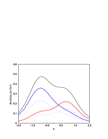
Figure 1: Negative helicity lepton distribution with $P_{A}(+)P_{B}(-)$

Some comments are in order for this result. Firstly, the main effect of QCD correction is just an enhancement of the tree level cross section: the $K$ factor is $1.5\sim 1.8$. It does not change significantly the shape of the lepton distributions. Secondly, the different contributions from $u(\bar{u})$ and $d(\bar{d})$ quarks can be understood intuitively by observing the following aspects: (1) The polarized quark distributions in the polarized proton $P(+)$ tell us,

$$u(\uparrow)\gg d(\downarrow)\sim u(\downarrow)\gg d(\uparrow)\gg\bar{u}(\uparrow,\downarrow)\sim\bar{d}(\uparrow,\downarrow)\ ,$$

where ${\uparrow},{\downarrow}$ mean the quark’s spin parallel and anti-parallel to the parent proton’s spin. This relation implies the dominant subprocesses for the $P_{A}(+)P_{B}(-)$ case to be (i) $u_{A}(\uparrow)\bar{u}_{B}$, (ii) $\bar{u}_{A}u_{B}(\uparrow)$, (iii) $d_{A}(\downarrow)\bar{d}_{B}$ and (iv) $\bar{d}_{A}d_{B}(\downarrow)$. (2) From the angular momentum conservation, the spin of produced $Z$ boson is aligned to $P_{A}$ ($P_{B}$) direction for $u_{A}\bar{u}_{B}$ and $\bar{u}_{A}u_{B}$ ($d_{A}\bar{d}_{B}$ and $\bar{d}_{A}d_{B}$) annihilations. Furthermore, it is well known that the negative (positive) helicity lepton from the $Z$ decay has higher probability to be produced in the opposite (same) direction of $Z$ boson’s spin. (3) The third point to be noted is that the $V-A$ coupling is larger than the $V+A$ coupling for the quark and $Z$ boson interaction. This suggests that among four subprocesses in (1), (ii) and (iii) eventually dominate the process. (4) Finally, since the momentum fractions of quarks are bigger than those of anti-quarks, the distributions of negative helicity lepton from (ii) and (iii) are Lorentz boosted to the negative and positive rapidity regions respectively.

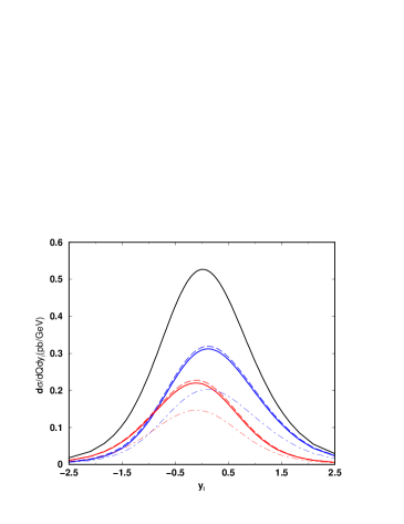
Figure 2: Positive helicity lepton distribution with $P_{A}(+)P_{B}(-)$

We plot in Fig.2 the positive helicity lepton distributions with $P_{A}(+)P_{B}(-)$ configuration. In this case, we do not see such a characteristic feature like one in Fig.1. The $u\bar{u}$ contribution slightly dominates the cross section.

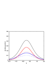
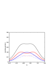
(3a)	(3b)

Figure 3: Lepton distribution with $P_{A}(+)P_{B}(+)$

Figs. 3a (3b) and 4a (4b) show lepton distributions with positive (negative) helicity for the $P_{A}(+)P_{B}(+)$ and $P_{A}(-)P_{B}(-)$ configurations. In the case of $P_{A}(+)P_{B}(+)$, $u\bar{u}$ and $d\bar{d}$ annihilations, roughly speaking, contribute similarly in size. For $P_{A}(-)P_{B}(-)$ annihilation, $u\bar{u}$ sub-process dominates the cross section. One can understand these behaviors again intuitively by noting the observation explained before concerning Fig.1.

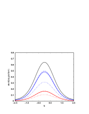
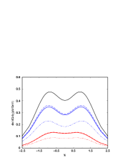
(4a)	(4b)

Figure 4: Lepton distribution with $P_{A}(-)P_{B}(-)$

We also estimate the lepton helicity asymmetry $A$ which is defined by,

$$A\equiv\frac{d\sigma(\lambda_{l}=-1)-d\sigma(\lambda_{l}=+1)}{d\sigma(\lambda_{l}=-1)+d\sigma(\lambda_{l}=+1)}$$

This asymmetry is plotted in Fig. 5 for the configuration of $P_{A}(+)P_{B}(-)$ using the various parton parameterizations in Refs.[7, 8].

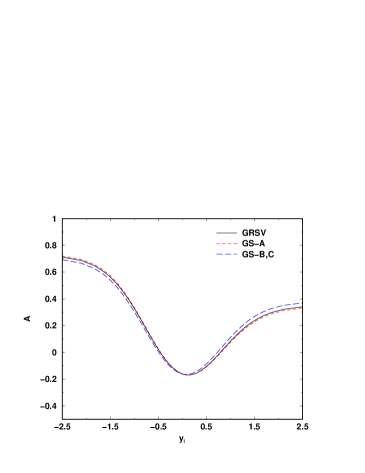
Figure 5: Helicity asymmetry distribution with $P_{A}(+)P_{B}(-)$

This asymmetry amounts to around 50%, but the dependence on the various parton parameterizations is quite weak. The reason is that the process is dominated by the quark and anti-quark annihilation in the RHIC energy region and the gluon initiated Compton subprocess, in which the ambiguity of gluon distribution will appear, gives a tiny correction to the cross section. This is already expected from also the fact that the QCD correction has mainly an enhancement effect of the tree level cross section.

Figs.6 show the same asymmetry for the case of $P_{A}(+)P_{B}(+)$ (6a) and $P_{A}(-)P_{B}(-)$ (6b).

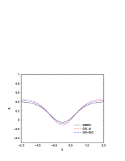
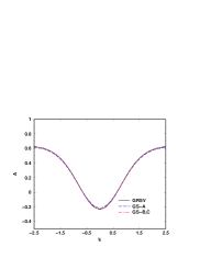
(6a)	(6b)

Figure 6: Helicity asymmetry distribution with $P_{A}(\pm)P_{B}(\pm)$

5 SUMMARY

We have presented the lepton helicity distributions in the polarized Drell-Yan process at the ${\cal O}(\alpha_{s})$ level in QCD. We have numerically analyzed the cross section on the $Z$ pole and pointed out that the $u(\bar{u})$ and $d(\bar{d})$ quarks give different and characteristic contributions to the lepton helicity distributions which deserve some theoretical interests. The QCD corrections mainly enhance the tree level cross sections and this fact can explain qualitatively the lepton helicity distributions from the various proton’s spin configurations.

We have also estimated the lepton helicity asymmetry which amounts to around 50%. Since the $q-\bar{q}$ subprocess is dominant in the RHIC energy region, we will not be able, unfortunately, to find difference between various parton parameterizations which have big ambiguities in the gluon distributions.

From the experimental point of view, it seems very difficult to measure the helicity of produced muon and/or electron from Drell-Yan process. However, if we can observe the $\tau$ lepton produced from the Drell-Yan process and its decay, we will be able to compare the experimental data and theoretical prediction.

We hope that various kinds of new experiments and theoretical investigations will be able to clarify not only perturbative and nonperturbative aspects of QCD but also the full structure of all interactions in Nature.

The work of J. K. is supported in part by the Monbu-kagaku-sho Grant-in-Aid for Scientific Research No. C-13640289.

References

- [1] G.Bunce, N.Saito, J.Soffer and W.Vogelsang, Ann. Rev. Nucl. Part. Sci. 50 (2000) 525.
-
[2]
A. Weber, Nucl. Phys. B382 (1992) 63.
T. Gehrmann, Nucl. Phys.B498 (1997) 245.
C. Bourrely and J. Soffer, Phys. Lett. B314 (1993) 132; Nucl. Phys. B423 (1994) 329.
B. Kamal, Phys. Rev. D57 (1998) 6663. -
[3]
J. P. Ralston and D.E. Soper Nucl. Phys. B152 (1979) 109.
R. L. Jaffe and X. Ji, Nucl. Phys. B375 (1992) 527.
D. Sivers, Phys. Rev. D51 (1995) 4880.
W. Vogelsang and A. Weber, Phys. Rev. D48 (1993) 2073.
A. P. Contogouris, B. Kamal and Z. Merebashvili, Phys. Lett. B337 (1994) 169. -
[4]
J. Kubar, M. Le Bellac, J.L.Meunier and G.Plaut,
Nucl. Phys. B175 (1980) 251.
W. Vogelsang and A. Weber, Phys. Rev. D48 (1993) 2073. - [5] See e.g. R.D.Field, Applications of Perturbative QCD (Frontiers in Physics, Vol.77), Harpercollins (Sd) (1989/06/01)
- [6] J. Kodaira and H. Yokoya, in preparation.
- [7] M. Glück, E. Reya, M. Stratmann and W. Vogelsang, Phys. Rev. D53 (1996) 4775.
-
[8]
A. D. Martin, R. G. Roberts, W. J. Stirling and R. S. Thorne,
Eur. Phys. J. C14 (2000) 133.
T. Gehrmann and W. J. Stirling, Phys. Rev. D53 (1996) 6100.