QCD two-loop amplitudes for $e^{+}e^{-}\to$ 3 jets: the fermionic contribution

Abstract

We review a new technique for the calculation of two-loop amplitudes and discuss as an example the fermionic contributions to $e^{+}e^{-}\to q\bar{q}g$.

1 Introduction

The construction of fully differential next-to-next-to-leading order (NNLO) programs is a challenging problem and urgently needed to match the accuracy reached in today’s collider experiments. While for inclusive observables like for example the total hadronic cross section in $e^{+}e^{-}$ annihilation the step from NLO to NNLO is far less demanding – and has been taken a long time ago – the contrary is true for less inclusive quantities as for example jet rates. Essentially one has to adress two problems in jet physics at NNLO accuracy. The first one is related to the fact that one needs to treat two-loop integrales with more than one scale. These integrals are much harder to solve than one-scale integrals. The second problem which needs to be solved is the combination of virtual and real corrections – which are separately infrarot (IR) divergent – into a IR finite cross section. Given these difficulties it is clear that only for specific reactions NNLO calculations can be envisaged. Important reactions for which one should go beyond the NLO approximation are for example: Bhabha scattering, $pp,p\bar{p}\rightarrow 2\;\mbox{jets}$, and $e^{+}e^{-}\rightarrow 3\;\mbox{jets}$. Among these examples the $e^{+}e^{-}$ annihilation into 3 jets is of particular interest. Historically this reaction was one of the first clean tests of Quantum Chromodynamics (QCD) as the theory of strong interaction. Today the 3-jet production in $e^{+}e^{-}$ annihilation is still an excellent laboratory for precise tests of QCD and jet physics. In particular $e^{+}e^{-}\to 3\;\mbox{jets}$ is also a perfect reaction for measureing the QCD coupling $\alpha_{s}$ with high accuracy. It is exactly here where the need for NNLO predictions for 3-jet production becomes most prominent: at present the measurements of $\alpha_{s}$ are plagued by scale uncertainties of the theoretical predictions [1]. These uncertainties arise from uncalculated higher order contributions. Although formally of higher order these uncertainties can still be large. They can be reduced only by a NNLO calculation. The residual scale dependence of the 3-jet rate $f_{3}$ can be studied using the following formula

$$f_{3}\left(y,{\mu^{2}\over s}\right) = {\alpha_{s}(\mu)\over 2\pi}{A(y)}$$ (1)

$$+\left({\alpha_{s}(\mu)\over 2\pi}\right)^{2}\*\left({B(y)}+{1\over 2}\*\beta_{0}\*\ln\left({\mu^{2}\over s}\right)\*{A(y)}\right)$$

$$+\left({\alpha_{s}(\mu)\over 2\pi}\right)^{3}\*\bigg{(}{C(y)}+\beta_{0}\*\ln\left({\mu^{2}\over s}\right)\*{B(y)}$$

$$+{1\over 4}\*\left[\beta_{0}^{2}\*\ln\left({\mu^{2}\over s}\right)^{2}+\beta_{1}\*\ln\left({\mu^{2}\over s}\right)\right]\*{A(y)}\bigg{)}.$$

Here $\beta_{0},\beta_{1}$ denote the coefficients of the QCD $\beta$-function, $y$ is the resolution of the jet algorithm and $A$, $B$, and $C$ are the LO, NLO, NNLO coefficients at $\mu^{2}=s$. The residual scale dependence is illustrated in fig. 1 for the Durham algorithm at $y=0.1$.

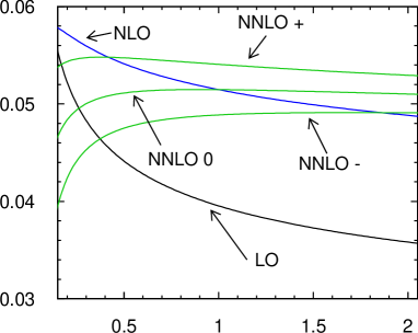
Figure 1: Residual scale dependence of $f_{3}(y,{\mu^{2}\over s})$.

For the NNLO curves three different scenarios have been assumed: one scenario in which the NNLO corrections vanish for $\mu^{2}=s$, and two scenarios where a $\pm$ 5 % correction at $\mu^{2}=s$ have been assumed. It is clearly visible that the NNLO corrections improves the residual scale dependence. For a 3-jet prediction at NNLO accuracy several ingredients are needed: First the matrix elements for $e^{+}e^{-}\to q\bar{q}ggg,\;q\bar{q}q^{\prime}\bar{q}^{\prime}\!g$ have to be evaluated. They are obtained from a leading-order calculation and are known for a long time [2, 3]. Second the one-loop matrix elements for $e^{+}e^{-}\to q\bar{q}gg,q\bar{q}q^{\prime}\bar{q}^{\prime}$ are needed. They have been calculated in refs. [4, 5, 6, 7]. Finally one needs the NNLO amplitudes for $e^{+}e^{-}\to q\bar{q}g$ [8, 9, 11, 10, 12]. In the following the calculation of fermionic contribution of the NNLO matrix elements is reported. One should keep in mind that the combination of these 3 ingredients into an infrared finite cross section is still a highly non-trivial – and so far unsolved – problem.

2 A new approach to calculate NNLO amplitudes

Due to the tremendous activities in the field enormous progress has been made in the past. All the relevant double box scalar integrals have been calculated [13, 14, 15, 16]. For a few reactions these results have been used to obtain NNLO scattering amplitudes [17, 18, 19, 20, 21, 22, 8, 23, 24, 25, 9, 26]. Today one can say that a standard approach to perform these calculations exist. Essentially it consists of three steps:

1. Generation of relevant Feynman diagrams.

2. Reduction of tensor integrals to scalar integrals via Schwinger parametrization [27, 28].

3. Reduction of scalar integrals with raised powers and in higher dimensions to master integrals via partial integration and Lorentz invariance equations [29, 30, 31].

The final result is than obtained in terms of master integrals. They have to be calculated analytically. The bottleneck of this approach is that one has to create and to solve a huge system of equations to obtain the desired reduction to master integrals. In contrast to the naive expectation, topologies which at first glance look not so difficult may involve much more work than the more complicated once. For example it is almost trivial to find the reduction scheme for the planar double box although the master integral itself is one of the most complicated once. In ref. [32] we have proposed a different method. The basic idea is that one applies only obvious reductions like for example the triangle rule. In particular one does not perform a complete reduction to master integrals. Instead one calculates the scalar integrals in higher dimensions and with raised powers of the propagators directly.

a)

b)

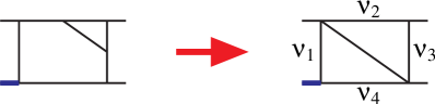
c)

Figure 2: Tensor reduction of the general pentabox topology a) to scalar integrals in higher dimensions and raised powers of the propagators b). Application of the triangle rule yielding the C-topology $\mbox{C}(m={d\over 2}+\epsilon,\nu_{1},\nu_{2},\nu_{3},\nu_{4},\nu_{5})$ c).

To illustrate the method let us consider the so-called penta-box. A corresponding Feynman diagram is shown in fig. 2a. Applying Schwinger parameterization one arrives at the scalar topology shown schematically in fig. 2b. An obvious application of the triangle rule allows the elimination of two propagators [33] (cf. fig. 2c). The resulting topology is often called C-topology. As mentioned earlier the C-topology appears in higher dimensions $(d=2m-2\epsilon,\;m\in N)$ and with raised powers of the propagators $(\nu_{1},\ldots,\nu_{5})$. In the approach advocated here an analytic expression for the C-topology is needed. Such an expression can be obtained in terms of infinite sums [32]. The generic structure is shown in eq. (2).

$$\mbox{C}(m={d\over 2}+\epsilon,\nu_{1},\ldots,\nu_{5})\sim\sum\limits_{i_{1}=0}^{\infty}\sum\limits_{i_{2}=0}^{\infty}\frac{x_{1}^{i_{1}}}{i_{1}!}\frac{x_{2}^{i_{2}}}{i_{2}!}\bigg{[}$$

$$x_{1}^{2m-2\epsilon-\nu_{1235}}x_{2}^{2m-2\epsilon-\nu_{2345}}{\Gamma(i_{1}+2m-2\epsilon-\nu_{125})\over\Gamma(i_{1}+1+2m-2\epsilon-\nu_{1235})}$$

$$\times\frac{\Gamma(i_{1}+i_{2}+2m-2\epsilon-\nu_{235})\Gamma(i_{2}+2m-2\epsilon-\nu_{345})}{\Gamma(i_{1}+i_{2}+4m-4\epsilon-\nu_{12345}-\nu_{5})}$$

$$\times\frac{\Gamma(i_{1}+i_{2}+3m-3\epsilon-\nu_{12345})}{\Gamma(i_{2}+1+2m-2\epsilon-\nu_{2345})}+\ldots\bigg{]}$$ (2)

It is obvious that such a representation is completely useless unless one is able to evaluate the $\epsilon$-expansion in terms of known functions. Fortunately this is possible using a few basic algorithms for nested sums [32]. The basic idea here is that one rewrites the sums using the relation

$$\sum\limits_{i=0}^{\infty}\sum\limits_{j=0}^{\infty}a_{ij}=a_{00}+\sum\limits_{j=1}^{\infty}a_{0j}+\sum\limits_{i=1}^{\infty}a_{i0}+\sum\limits_{n=1}^{\infty}\sum\limits_{j=1}^{n-1}a_{j(n-j)}.$$ (3)

Furthermore one can expand the $\Gamma$-functions by the means of

$${\Gamma(-n+\epsilon)} = {(-1)^{n}\over\epsilon n!}{\Gamma(1+\epsilon)}(1+S_{1}(n)\epsilon$$ (4)

$$+S_{1,1}(n)\epsilon^{2}+S_{1,1,1}(n)\epsilon^{3}+S_{1,1,1,1}(n)\epsilon^{4}+\ldots$$

and related identities [34]. Here $S_{1,\ldots}(n)$ denote the harmonic sums, see e.g. ref. [34]. Inspecting the sums which appear using eq. (3) and eq. (4) one observes that the algorithms needed are just a generalization of the algorithms studied in ref. [34]. In particular defining the nested sums as a generalization of the harmonic sums by

$$S(n;m_{1},...,m_{k};x_{1},...,x_{k})=\sum\limits_{i_{1}=1}^{n}\sum\limits_{i_{2}=1}^{i_{1}}\cdots\sum\limits_{i_{k}=1}^{i_{k-1}}{{x_{1}^{i_{1}}\over i_{1}^{m_{1}}}\cdots{x_{k}^{i_{k}}\over i_{k}^{m_{k}}}}$$

$$=\sum\limits_{i=1}^{n}{{\frac{x_{1}^{i}}{i^{m_{1}}}}}S({{i}};m_{2},...,m_{k};x_{2},...,x_{k})$$ (5)

the following four basic operations are sufficient to evaluate the $\epsilon$-expansion of the C-topology in terms of multiple polylogarithms [35]:

1. Multiplication

   $${{S(n;m_{1},...;x_{1},...)\,\times\,S(n;m_{1}^{\prime},...;x_{1}^{\prime},...)}}$$ (6)

2. Sums involving $i$ and $n-i$:

   $$\sum\limits_{i=1}^{n-1}\frac{x_{1}^{i}}{i^{m_{1}}}S({{i}};m_{2}...;x_{2},...)$$

   $$\times\frac{{x_{1}^{\prime}}^{n-i}}{(n-i)^{m_{1}^{\prime}}}S({{n-i}};m_{2}^{\prime},...;x_{2}^{\prime},...)$$ (7)

3. Conjugations:

   $$\sum\limits_{i=1}^{n}{{\left(\begin{array}[]{c}n\\ i\\ \end{array}\right)(-1)^{i}}}\frac{x_{0}^{i}}{i^{m_{0}}}S(i;m_{1},...,m_{k};x_{1},...,x_{k})$$ (8)

4. Sums involving binomials and $n-i$:

   $$\sum\limits_{i=1}^{n-1}{{\left(\begin{array}[]{c}n\\ i\\ \end{array}\right)}}\left(-1\right)^{i}\frac{x_{1}^{i}}{i^{m_{1}}}S(i;m_{2}...;x_{2},...)$$ (11)

   $$\times\frac{{x_{1}^{\prime}}^{n-i}}{(n-i)^{m_{1}^{\prime}}}S({{n-i}};m_{2}^{\prime},...;x_{2}^{\prime},...)$$ (12)

In ref. [32] we have given explicit algorithms for the four basic operations. For their implementation we used Form3 [36] and Ginac [37, 38]. Using these programs we calculated more than 300 C-topologies analytically. In particular we have checked that our results for the two master integrals ${\rm C}(2,1,1,1,1,1),{\rm C}(2,1,1,1,1,2)$ agree with those given in ref. [39]. All the simpler topologies can be calculated in the same way.

3 Results

The amplitude ${\cal A}_{\gamma}$ for the process $e^{+}e^{-}\to\gamma^{\ast}\to q({p_{1}})g({p_{2}})\bar{q}({p_{3}})$ can be written as a leptonic part $L_{\mu}$ multiplied by a hadronic part $H_{\mu}$:

$${\cal A}_{\gamma} \sim {1\over s}\,H_{\mu}\,L^{\mu}$$ (13)

$$={1\over s}\,g_{s}(H_{\mu}^{(0)}+{\alpha_{s}\over 2\pi}H_{\mu}^{(1)}+\left({\alpha_{s}\over 2\pi}\right)^{2}H_{\mu}^{(2)}+\ldots)\,L^{\mu},$$

with $s=({p_{1}}+{p_{2}}+{p_{3}})^{2}$ and $g_{s}=\sqrt{4\pi\alpha_{s}}$. Furthermore the hadronic part can be decomposed according to the colour structure. In particular we have

$$H_{\mu}^{(2)} = T^{a}_{q\bar{q}}\bigg{(}N^{2}H_{2,\mu}^{(2)}+H_{0,\mu}^{(2)}+{1\over N^{2}}H_{-2,\mu}^{(2)}$$ (14)

$$+ {n_{f}NH_{n_{f},1,\mu}^{(2)}+{n_{f}\over N}H_{n_{f},-1,\mu}}^{(2)}+n_{f}^{2}H_{n_{f}^{2},\mu}^{(2)}$$

$$+ \Sigma_{f}\left({4\over N}-N\right)H_{\Sigma_{f},\mu}^{(2)}\bigg{)},$$

with $T^{a}_{q\bar{q}}$ the generator of the $SU(N)$ gauge group and $n_{f}$ the number of massless quarks. In this talk we discuss only the contributions proportional to $n_{f}N$ and ${n_{f}\over N}$. The hadronic contribution can also be decomposed according to the spinor structure:

$$H_{\mu} = c_{1}\*{1\over s}\*\langle{p_{1}}|{/\!\!\!\!\!{p_{2}}}|{p_{3}}\rangle\*{\epsilon_{g}}_{\mu}$$ (15)

$$+\ldots+c_{4}\*{1\over s^{2}}\*\langle{p_{1}}|{/\!\!\!\!\!{p_{2}}}|{p_{3}}\rangle\*(\epsilon_{g}\cdot{p_{1}})\*{p_{1}}_{\mu}+\ldots$$

$$+c_{13}\*{1\over s^{2}}\*\langle{p_{1}}|{/\!\!\!\!\!{p_{2}}}|{p_{3}}\rangle\*(\epsilon_{g}\cdot{p_{3}})\*{p_{2}}_{\mu}$$

where the functions $c_{1}-c_{13}$ depend only on the ratios $x_{1}=2({p_{1}}\cdot{p_{2}})/s$, $x_{2}=2({p_{2}}\cdot{p_{3}})/s$. Due to various constraints arising from gauge invariance or quark anti-quark antisymmetry only 4 of them are needed. All the remaining ones can be expressed in terms of these 4 functions which we chose to be $c_{2},\,c_{4},\,c_{6}$ and $c_{12}$. The perturbative expansion in $\alpha_{s}$ of the functions $c_{i}$ is defined through

$$c_{i}=g_{s}\left(c_{i}^{(0)}\!+\left(\frac{\alpha_{s}}{2\pi}\right)c_{i}^{(1)}\!+\left(\frac{\alpha_{s}}{2\pi}\right)^{2}c_{i}^{(2)}\!+O(\alpha_{s}^{3})\right)\!\!.$$ (16)

Using the methods described in the previous section we calculated all the 13 functions and used the constraints as a check of our calculation. Furthermore we checked the structure of the ultraviolet as well as the infrared divergencies [40, 41]. Note that the general structure of the IR divergencies as conjectured in ref. [40] has been proven recently by Sterman and Tejeda-Yeomans [41]. We have also compared our results with results published recently [8, 9]. In refs. [8, 9] the result is written in terms of 2-dimensional harmonic polylogarithms instead of the multiple polylogarithms used here. Expressing the 2-dimensional harmonic polylogarithms in terms of multiple polylogarithms we found complete agreement for the $n_{f}N$ and ${n_{f}\over N}$ contribution calculated here.

Following ref. [9] we used the general structure of the infrared divergencies as described by Catani [40] to define the finite parts of the coefficients $c_{i}$:

$$c_{i}^{(2),\mbox{\scriptsize\rm fin}} = c_{i}^{(1),\mbox{\scriptsize\rm ren}}-{\bf I}^{(1)}(\epsilon)c_{i}^{(1),\mbox{\scriptsize\rm ren}}-{\bf I}^{(2)}(\epsilon)c_{i}^{(0)}\,,$$ (17)

with the one- and two-loop insertion operators ${\bf I}^{(1)}(\epsilon)$ and ${\bf I}^{(2)}(\epsilon)$ given in ref. [40]. As an example, we present the result for the $n_{f}N$-contribution to the finite part $c_{4}^{(2),\mbox{\scriptsize\rm fin}}$ at two loops,

$$c_{4}^{(2),\mbox{\scriptsize\rm fin}}({x_{1}},{x_{2}})\bigg{|}_{n_{f}N}=n_{f}\*N\*\bigg{(}-{19\over 18}\*{1\over{x_{1}}\*(1-{x_{2}})}$$

$$+{1\over 36}\*{\ln({x_{2}})\over(1-{x_{2}})}\*\bigg{[}36\*{(1+{x_{1}})\over({x_{1}}+{x_{2}})}-{59\over{x_{1}}}-{50\over{x_{1}}\*(1-{x_{2}})}$$

$$+12\*{(1-3\*{x_{1}})\*(1-{x_{1}})\over{x_{1}}\*(1-{x_{1}}-{x_{2}})}\bigg{]}+{({x_{1}}-{x_{2}})\over({x_{1}}+{x_{2}})^{3}}\*{\rm R_{1}}({x_{1}},{x_{2}})$$

$$-\bigg{[}{5\over 12}\*{(2-{x_{2}})\over{x_{1}}\*(1-{x_{2}})^{2}}+{2\over({x_{1}}+{x_{2}})^{2}}\bigg{]}\*{{\rm Li}_{2}(1-{x_{2}})}$$

$$+{1\over 4}\*{(2-{x_{2}})\over{x_{1}}\*(1-{x_{2}})^{2}}\*\bigg{[}\ln({x_{2}})^{2}+{1\over 3}\*{\zeta_{2}}\bigg{]}$$

$$-{1\over 12}\*{(7\*{x_{1}}-5\*{x_{2}}-6\*{x_{1}}\*{x_{2}}+5\*{x_{2}}^{2}+{x_{1}}^{2})\over(1-{x_{2}})\*{x_{1}}\*(1-{x_{1}}-{x_{2}})\*({x_{1}}+{x_{2}})}\*\ln({x_{1}})$$

$$-{{\rm R}({x_{1}},{x_{2}})\over(1-{x_{1}}-{x_{2}})\*(1-{x_{2}})\*({x_{1}}+{x_{2}})}\*\bigg{[}{17\over 6}\*{x_{2}}-{35\over 12}\*{x_{1}}$$

$$-{19\over 12}+{1\over 12}\*{(1+{x_{1}})\over(1-{x_{2}})}-{1\over 3}\*{(1-3\*{x_{1}})\*(1-{x_{1}})\over(1-{x_{1}}-{x_{2}})}$$

$$+{5\*{x_{2}}^{2}\over 12\*{x_{1}}}-{5\over 6}\*{{x_{2}}\over{x_{1}}}+2\*{{x_{1}}\*(1+{x_{1}})\over({x_{1}}+{x_{2}})}\bigg{]}$$

$$-\bigg{[}{1\over 12}\*{(2-{x_{2}})\over{x_{1}}\*(1-{x_{2}})^{2}}-{2\over({x_{1}}+{x_{2}})^{2}}\bigg{]}\*{{\rm Li}_{2}(1-{x_{1}})}\bigg{)}$$

$$-i\*\pi\*n_{f}\*N\*\bigg{(}{(2-{x_{2}})\*\ln({x_{2}})\over 2\*{x_{1}}\*(1-{x_{2}})^{2}}+{1\over 2}\*{1\over{x_{1}}\*(1-{x_{2}})}\bigg{)}.$$ (18)

We have introduced the function ${\rm R}({x_{1}},{x_{2}})$ defined in [42]. In addition, it is convenient, to define the symmetric function ${\rm R_{1}}({x_{1}},{x_{2}})$, which contains a particular combination of multiple polylogarithms [35],

$${\rm R_{1}}({x_{1}},{x_{2}})=\bigg{(}\ln({x_{1}}){\rm Li}_{1,1}\left({{x_{1}}\over{x_{1}}\!+\!{x_{2}}},{x_{1}}\!+\!{x_{2}}\right)$$

$$-{1\over 2}{\zeta_{2}}\ln(1\!-\!{x_{1}}\!-\!{x_{2}})-{1\over 2}\ln({x_{1}})\ln({x_{2}})\ln(1\!-\!{x_{1}}\!-\!{x_{2}})$$

$$-\ln({x_{1}}){\rm Li}_{2}({x_{1}}\!+\!{x_{2}})-{\rm Li}_{1,2}\left({{x_{1}}\over{x_{1}}\!+\!{x_{2}}},{x_{1}}\!+\!{x_{2}}\right)$$

$$-{\rm Li}_{2,1}\left({{x_{1}}\over{x_{1}}\!+\!{x_{2}}},{x_{1}}\!+\!{x_{2}}\right)+{\rm Li}_{3}({x_{1}}\!+\!{x_{2}})\bigg{)}+({x_{1}}\leftrightarrow{x_{2}})\,.$$

All the multiple polylogarithms have simple arguments. As a consequence it is straightforward to obtain the analytic continuation, which can be used for the crossing of the amplitude.

4 Conclusion

In this talk we have presented the calculation of a specific colour structure of the QCD two-loop amplitude $e^{+}e^{-}\to q\bar{q}g$. The computation has been done by a completely new method [32]. The new approach provides a very efficient method for two-loop calculations. The tools developed in this approach can also be used for a systematic expansion of generalized hypergeometric functions. In addition the presented results provide an important cross check on recently obtained results [8, 9].

References

• [1] S. Bethke, (2002), hep-ex/0211012,
• [2] F.A. Berends, W.T. Giele and H. Kuijf, Nucl. Phys. B321 (1989) 39,
• [3] K. Hagiwara and D. Zeppenfeld, Nucl. Phys. B313 (1989) 560,
• [4] Z. Bern etΒ al., Nucl. Phys. B489 (1997) 3,
• [5] Z. Bern, L.J. Dixon and D.A. Kosower, Nucl. Phys. B513 (1998) 3,
• [6] E.W.N. Glover and D.J. Miller, Phys. Lett. B396 (1997) 257,
• [7] J.M. Campbell, E.W.N. Glover and D.J. Miller, Phys. Lett. B409 (1997) 503,
• [8] L.W. Garland etΒ al., Nucl. Phys. B627 (2002) 107,
• [9] L.W. Garland etΒ al., (2002), hep-ph/0206067,
• [10] S. Moch, P. Uwer and S. Weinzierl, (2002), hep-ph/0210009,
• [11] S. Moch, P. Uwer and S. Weinzierl, (2002), hep-ph/0207167,
• [12] S. Moch, P. Uwer and S. Weinzierl, (2002), hep-ph/0207043,
• [13] V.A. Smirnov, Phys. Lett. B460 (1999) 397,
• [14] J.B. Tausk, Phys. Lett. B469 (1999) 225,
• [15] V.A. Smirnov, Phys. Lett. B491 (2000) 130,
• [16] V.A. Smirnov, Phys. Lett. B500 (2001) 330,
• [17] Z. Bern, L.J. Dixon and D.A. Kosower, JHEP 01 (2000) 027,
• [18] C. Anastasiou etΒ al., Nucl. Phys. B601 (2001) 318,
• [19] C. Anastasiou etΒ al., Nucl. Phys. B601 (2001) 341,
• [20] C. Anastasiou etΒ al., Phys. Lett. B506 (2001) 59,
• [21] C. Anastasiou etΒ al., Nucl. Phys. B605 (2001) 486,
• [22] E.W.N. Glover, C. Oleari and M.E. Tejeda-Yeomans, Nucl. Phys. B605 (2001) 467, hep-ph/0102201,
• [23] Z. Bern, L.J. Dixon and A. Ghinculov, Phys. Rev. D63 (2001) 053007,
• [24] Z. Bern, A. DeΒ Freitas and L.J. Dixon, JHEP 09 (2001) 037,
• [25] Z. Bern, A. DeΒ Freitas and L. Dixon, JHEP 03 (2002) 018,
• [26] C. Anastasiou, E.W.N. Glover and M.E. Tejeda-Yeomans, Nucl. Phys. B629 (2002) 255,
• [27] O.V. Tarasov, Phys. Rev. D54 (1996) 6479,
• [28] O.V. Tarasov, Nucl. Phys. B502 (1997) 455,
• [29] G. ’tΒ Hooft and M.J.G. Veltman, Nucl. Phys. B44 (1972) 189,
• [30] K.G. Chetyrkin and F.V. Tkachov, Nucl. Phys. B192 (1981) 159,
• [31] T. Gehrmann and E. Remiddi, Nucl. Phys. B580 (2000) 485,
• [32] S. Moch, P. Uwer and S. Weinzierl, J. Math. Phys. 43 (2002) 3363,
• [33] C. Anastasiou, E.W.N. Glover and C. Oleari, Nucl. Phys. B575 (2000) 416,
• [34] J.A.M. Vermaseren, Int. J. Mod. Phys. A14 (1999) 2037,
• [35] A.B. Goncharov, Math. Res. Lett. 5 (1998) 497.
• [36] J.A.M. Vermaseren, (2000), math-ph/0010025,
• [37] C. Bauer, A. Frink and R. Kreckel, J. Symbolic Computation 33 (2002), cs/0004015,
• [38] S. Weinzierl, Comput. Phys. Commun. 145 (2002) 357,
• [39] T. Gehrmann and E. Remiddi, Nucl. Phys. B601 (2001) 248,
• [40] S. Catani, Phys. Lett. B427 (1998) 161,
• [41] G. Sterman, M.E. Tejeda-Yeomans, (2002), hep-ph/0210130,
• [42] R.K. Ellis, D.A. Ross and A.E. Terrano, Nucl. Phys. B178 (1981) 421.