Global Fits of Parton Distributions

1 Introduction

The fundamental quantities one requires in the calculation of scattering processes involving hadronic particles are the parton distributions. Global fits MRST2001 -ZEUSfit use all available data, largely structure functions, and the most up-to-date QCD calculations, currently NLO–in–$\alpha_{s}(Q^{2})$, to best determine these parton distributions and their consequences. In the global fits input partons are parameterized as, e.g.

$$xf(x,Q_{0}^{2})=(1-x)^{\eta}(1+\epsilon x^{0.5}+\gamma x)x^{\delta}$$

at some low scale $Q_{0}^{2}\sim 1-5{\rm GeV}^{2}$, and evolved upwards using NLO DGLAP equations. Perturbation theory should be valid if $Q^{2}>2{\rm GeV^{2}}$, and hence one fits data for scales above $2-5{\rm GeV}^{2}$, and this cut should also remove the influence of higher twists, i.e. power-suppressed contributions.

In principle there are many different parton distributions – all quarks and antiquarks and the gluons. However, $m_{c},m_{b}\gg\Lambda_{{\rm QCD}}$ (and top does not usually contribute), so the heavy parton distributions are determined perturbatively. Also we assume $s=\bar{s}$, and that isospin symmetry holds, i.e. $p\to n$ leads to $d(x)\to u(x)$ and $u(x)\to d(x)$. This leaves 6 independent combinations. Relating $s$ to $1/2(\bar{u}+\bar{d})$ we have the independent distributions

$$u_{V}=u-\bar{u},\quad d_{V}=d-\bar{d},\quad{\rm sea}=2*(\bar{u}+\bar{d}+\bar{s}),\quad\bar{d}-\bar{u},\quad g.$$

It is also convenient to define $\Sigma=u_{V}+d_{V}+{\rm sea}+(c+\bar{c})+(b+\bar{b})$. There are then various sum rules constraining parton inputs and which are conserved by evolution order by order in $\alpha_{S}$, i.e. the number of up and down valence quarks and the momentum carried by partons (the latter being an important constraint on the gluon which is only probed indirectly),

$$\int_{0}^{1}x\Sigma(x)+xg(x)\,dx=1.$$

When extracting partons one needs to consider that not only are there 6 independent combinations, but there is also a wide distribution of $x$ from $0.75$ to $0.00003$. One needs many different types of experiment for a full determination. The sets of data usually used are: H1 and ZEUS $F^{p}_{2}(x,Q^{2})$ data H1A ; ZEUS which covers small $x$ and a wide range of $Q^{2}$; E665 $F^{p,d}_{2}(x,Q^{2})$ data E665 at medium $x$; BCDMS and SLAC $F^{p,d}_{2}(x,Q^{2})$ data BCDMS -SLAC at large $x$; NMC $F^{p,d}_{2}(x,Q^{2})$ NMC at medium and large $x$; CCFR $F^{\nu(\bar{\nu})p}_{2}(x,Q^{2})$ and $F^{\nu(\bar{\nu})p}_{3}(x,Q^{2})$ data CCFR at large $x$ which probe the singlet and valence quarks independently; ZEUS and H1 $F^{p}_{2,charm}(x,Q^{2})$ data ZEUSc ; H1c ; E605 $pN\to\mu\bar{\mu}+X$ E605 constraining the large $x$ sea; E866 Drell-Yan asymmetry E866 which determines $\bar{d}-\bar{u}$; CDF W-asymmetry data Wasymm which constrains the $u/d$ ratio at large $x$; CDF and D0 inclusive jet data D0 ; CDF which tie down the high $x$ gluon; and NuTev Dimuon data NuTeV which constrain the strange sea.

The quality of the fit to data is usually determined by the $\chi^{2}$. There are various alternatives for calculating this. The simplest is adding statistical and systematic errors in quadrature. This ignores the correlations between data points, but it is the only available method for many data sets. In principle it should be improved upon, but in practice sometimes works perfectly well.

A more sophisticated approach is to use the covariance matrix

$$C_{ij}=\delta_{ij}\sigma_{i,stat}^{2}+\sum_{k=1}^{n}\rho^{k}_{ij}\sigma_{k,i}\sigma_{k,j},$$

where $k$ runs over each source of correlated systematic error and $\rho^{k}_{ij}$ are the correlation coefficients. The $\chi^{2}$ is defined by

$$\chi^{2}=\sum_{i=1}^{N}\sum_{j=1}^{N}(D_{i}-T_{i}(a))C^{-1}_{ij}(D_{j}-T_{j}(a)),$$

where $N$ is the number of data points, $D_{i}$ is the measurement and $T_{i}(a)$ is the theoretical prediction depending on parton input parameters $a$. Unfortunately, this relies on inverting large matrices.

One can also minimize with respect to the systematic errors, i.e. incorporate the systematic errors into the theory prediction

$$f_{i}(a,s)=T_{i}(a)+\sum_{k=1}^{n}s_{k}\Delta_{ik},$$

where $\Delta_{ik}$ is the one-sigma correlated error for point $i$ from source $k$. In this case the $\chi^{2}$ is defined by

$$\chi^{2}=\sum_{i=1}^{N}\biggl{(}\frac{D_{i}-f_{i}(a,s)}{\sigma_{i,unc}}\biggr{)}^{2}+\sum_{k=1}^{n}s_{k}^{2},$$

where the second term constrains the values of $s_{k}$. This allows the data to move en masse relative to the theory, but assumes the correlated systematic errors are Gaussian distributed. One can actually solve for each of the $s_{k}$ analytically CTEQLag , simplifying greatly. This method is identical to the correlation matrix definition of $\chi^{2}$ at the minimum, but it has the double advantage that smaller matrices need inverting and one sees explicitly the shift of data relative to theory. However, one may ask whether Gaussian correlated errors are realistic and whether it is valid to move data to compensate for the shortcomings of theory. MRST find that for HERA data increments in $\chi^{2}$ using this method are much the same as for adding errors in quadrature, and data move towards theory MRST2001 . However, for Tevatron jet data the correlated systematic errors dominate and must be incorporated properly.

Once a decision about $\chi^{2}$ is made, the above procedure completely determines parton distributions at present. The total fit is reasonably good and that for CTEQ6 CTEQ6 is shown in Table 1 for the large data sets. The total $\chi^{2}=1954/1811$. For MRST The total $\chi^{2}=2328/2097$ – but the errors are treated differently, and different data sets and cuts are used. The same sort of conclusion is true for other global fits Botje ; Giele ; Alekhin ; H1Krakow ; ZEUSfit (which use fewer data). However, there are some areas where the theory perhaps needs to be improved, as we will discuss later.

Table 1: Quality of fit to data for CTEQ6M

Data Set	no. of data	$\chi^{2}$
H1 $ep$	230	228
ZEUS $ep$	229	263
BCDMS $\mu p$	339	378
BCDMS $\mu d$	251	280
NMC $\mu p$	201	305
E605 (Drell-Yan)	119	95
D0 Jets	90	65
CDF Jets	33	49

2 Parton Uncertainties

2.1 Hessian (Error Matrix) approach

In this one defines the Hessian matrix $H$ by

$$\chi^{2}-\chi_{min}^{2}\equiv\Delta\chi^{2}=\sum_{i,j}H_{ij}(a_{i}-a_{i}^{(0)})(a_{j}-a_{j}^{(0)}).$$

$H$ is related to the covariance matrix of the parameters by $C_{ij}(a)=\Delta\chi^{2}(H^{-1})_{ij},$ and one can use the standard formula for linear error propagation.

$$(\Delta F)^{2}=\Delta\chi^{2}\sum_{i,j}\frac{\partial F}{\partial a_{i}}(H)^{-1}_{ij}\frac{\partial F}{\partial a_{j}},$$

This has been employed to find partons with errors by Alekhin Alekhin and H1 H1Krakow (each with restricted data sets), as demonstrated in Fig. 1.

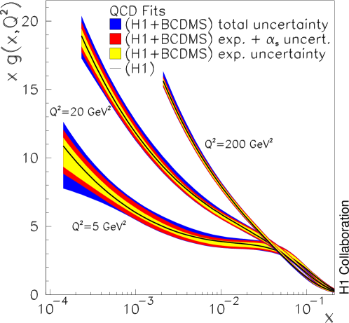
Figure 1: H1 determination of the gluon from their own data + BCDMS data with an emphasis on $g(x,Q^{2})$ and $\alpha_{S}(M_{Z}^{2})$ in the fit

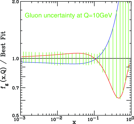
Figure 2: Results of CTEQ Hessian approach for the gluon uncertainty

The simple method can be problematic with larger data sets and numbers of parameters due to extreme variations in $\Delta\chi^{2}$ in different directions in parameter space. This is solved by finding and rescaling the eigenvectors of $H$ (CTEQ CTEQmul ; CTEQHes ; CTEQ6 ) leading to the diagonal form

$$\Delta\chi^{2}=\sum_{i}z_{i}^{2}.$$

The uncertainty on a physical quantity is then given by

$$(\Delta F)^{2}=\sum_{i}\bigl{(}F(S_{i}^{(+)})-F(S_{i}^{(-)})\bigr{)}^{2},$$

where $S_{i}^{(+)}$ and $S_{i}^{(-)}$ are PDF sets displaced along eigenvector directions by a given $\Delta\chi^{2}$. Similar eigenvector parton sets have also been introduced by MRST MRSTnew . However, there is an art in choosing the “correct” $\Delta\chi^{2}$ given the complication of the errors in the full fit THJPG . Ideally $\Delta\chi^{2}=1$, but this leads to unrealistic errors. CTEQ choose $\Delta\chi^{2}\sim 100$, which is perhaps conservative. MRST choose $\Delta\chi^{2}\sim 50$. An example of results is shown in Fig. 2.

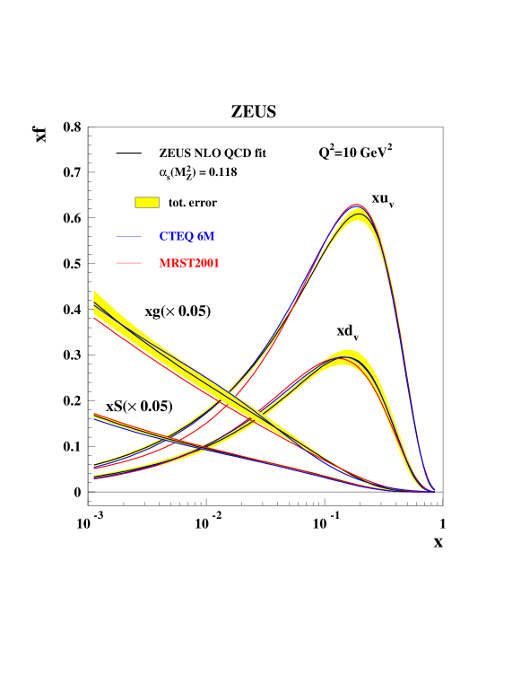
Figure 3: Parton densities and their errors extracted by fits by ZEUS

2.2 Offset method

In this the best fit is obtained by minimizing

$$\chi^{2}=\sum_{i=1}^{N}\biggl{(}\frac{(D_{i}-T_{i}(a))}{\sigma_{i,unc}}\biggr{)}^{2},$$

i.e. the best fit and parameters $a_{0}$ are obtained using only uncorrelated errors, forcing the theory to be close to unshifted data. The quality of the fit is estimated by adding errors in quadrature. The systematic errors on the $a_{i}$ are determined by letting each $s_{k}=\pm 1$ and adding the deviation in quadrature, or equivalently by calculating 2 Hessian matrices

$$M_{ij}=\frac{\partial^{2}\chi^{2}}{\partial a_{i}\partial a_{j}}\qquad V_{ij}=\frac{\partial^{2}\chi^{2}}{\partial a_{i}\partial s_{j}},$$

and defining covariance matrices

$$C_{stat}=M^{-1}\qquad C_{sys}=M^{-1}VV^{T}M^{-1}\qquad C_{tot}=C_{stat}+C_{sys},$$

which is used in practice. This was used in early H1 Zomer and ZEUS Botje fits. It is still used by ZEUS ZEUSfit , as shown in Fig. 3, and is a conservative approach to systematic errors leading to a bigger uncertainty for a given $\Delta\chi^{2}$.

2.3 Statistical Approach

In principle one constructs an ensemble of distributions labelled by ${\cal F}$ each with probability $P(\{{\cal F}\})$, where one can incorporate the full information about measurements and their error correlations into the calculation of $P(\{{\cal F}\})$. This is statistically correct, and does not rely on the approximation of linear propagation errors in calculating observables. However, it is inefficient, and in practice one generates $N_{pdf}$ ($N_{pdf}$ can be as low as $100$) different distributions with unit weight but distributed according to $P(\{{\cal F}\})$ Giele . Then the mean $\mu_{O}$ and deviation $\sigma_{O}$ of an observable $O$ are given by

$$\mu_{O}=\frac{1}{N_{pdf}}\sum_{1}^{N_{pdf}}O(\{{\cal F}\}),\quad\sigma_{O}^{2}=\frac{1}{N_{pdf}}\sum_{1}^{N_{pdf}}(O(\{{\cal F}\})-\mu_{O})^{2}.$$

Currently this approach uses only proton DIS data sets in order to avoid complicated uncertainty issues, e.g. shadowing effects for nuclear targets, and also demands consistency between data sets. However, it is difficult to find many truly compatible DIS experiments, and consequently the Fermi2001 partons are determined by only H1, BCDMS, and E665 data sets. They result in good predictions for many Tevatron cross-sections. However, the restricted data sets mean there is restricted information – data sets are deemed either perfect or, in the case of most of them, useless – leading to unusual values for some parameters. e.g. $\alpha_{S}(M_{Z}^{2})=0.112\pm 0.001$ and a very hard $d_{V}(x)$ at high $x$ (together these facilitate a good fit to Tevatron jets independent of the high-$x$ gluon). These partons would produce some extreme predictions. Nevertheless, the approach does demonstrate that the Gaussian approximation is often not good, and therefore highlights shortcomings in the methods outlined in the previous sections. It is a very attractive, but ambitious large-scale project, still in need of some further development, in particular the inclusion of a wider variety of data.

2.4 Lagrange Multiplier method

This was first suggested by CTEQ CTEQLag and has been concentrated on by MRST MRSTnew . One performs the fit while constraining the value of some physical quantity, i.e. one minimizes

$$\Psi(\lambda,a)=\chi^{2}_{global}(a)+\lambda F(a)$$

for various values of $\lambda$. This gives a set of best fits for particular values of the quantity $F(a)$ without relying on the quadratic approximation for $\chi^{2}$. The uncertainty is then determined by deciding an allowed range of $\Delta\chi^{2}$. One can also easily check the variation in $\chi^{2}$ for each of the experiments in the global fit and ascertain if the total $\Delta\chi^{2}$ is coming specifically from one region, which might cause concern. In principle, this is superior to the Hessian approach, but it must be repeated for each physical process.

2.5 Results

I choose the cross-section for $W$ and Higgs production at the Tevatron and LHC (for $M_{H}=115{\rm GeV}$) as examples. Using their fixed value of $\alpha_{S}(M_{Z}^{2})=0.118$ and $\Delta\chi^{2}=100$ CTEQ obtain

$$\Delta\sigma_{W}(\rm LHC)\approx\pm 4\%\quad\Delta\sigma_{W}({\rm Tev})\approx\pm 5\%\quad\Delta\sigma_{H}({\rm LHC})\approx\pm 5\%.$$

Using a slightly wider range of data, $\Delta\chi^{2}\sim 50$ and $\alpha_{S}(M_{Z}^{2})=0.119$ MRST obtain

$$\Delta\sigma_{W}(\rm Tev)\approx\pm 1.2\%\quad\Delta\sigma_{W}({\rm LHC})\approx\pm 2\%$$

$$\Delta\sigma_{H}(\rm Tev)\approx\pm 4\%\quad\Delta\sigma_{H}({\rm LHC})\approx\pm 2\%.$$

MRST also allow $\alpha_{S}(M_{Z}^{2})$ to be free. In this case $\Delta\sigma_{W}$ is quite stable but $\Delta\sigma_{H}$ almost doubles. Contours of variation in $\chi^{2}$ for predictions of these cross-sections are shown in Fig. 4.

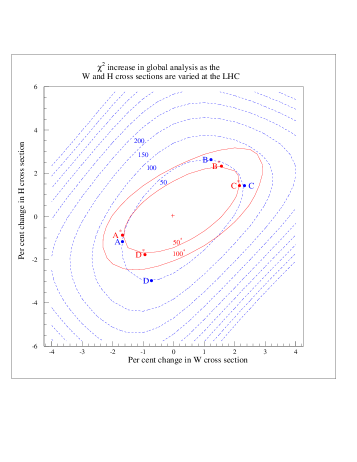
Figure 4: $\chi^{2}$-plot for $W$ and Higgs production at the Tevatron (left) and LHC (right) with $\alpha_{S}$ free and fixed at $\alpha_{S}=0.119$

Hence, the estimation of uncertainties due to experimental errors has many different approaches and different types and amount of data actually fit. Overall the uncertainty from this source is rather small – only more than a few $\%$ for quantities determined by the high $x$ gluon and very high $x$ down quark. However, different approaches can lead to rather different central values, as illustrated for determinations of $\alpha_{S}(M_{Z}^{2})$ in Table 2. This shows that there are other matters to consider. As well as the experimental errors on data we need to determine the effect of assumptions made about the fit, e.g. cuts made on the data, the data sets fit, the parameterization for input sets, the form of the strange sea, etc.. Many of these can be as important as the errors on the data used (or more so). This is demonstrated in Fig. 5 which shows the predictions for $W$ and Higgs production at the Tevatron from MRST2001 and CTEQ6. As well as the consequences of these assumptions we must also consider the related problem of theoretical errors.

Table 2: Values of $\alpha_{s}(M_{Z}^{2})$ and its error from different NLO QCD fits

Group	$\Delta\chi^{2}$	$\alpha_{S}(M_{Z}^{2})$
CTEQ6	$\Delta\chi^{2}=100$	$0.1165\pm 0.0065(exp)$
ZEUS	$\Delta\chi_{eff}^{2}=50$	$0.1166\pm 0.0049(exp)\pm 0.0018(model)$ $\pm 0.004(theory)$
MRST01	$\Delta\chi^{2}=20$	$0.1190\pm 0.002(exp)\pm 0.003(theory)$
H1	$\Delta\chi^{2}=1$	$0.115\pm 0.0017(exp)^{+~{}~{}0.0009}_{-~{}~{}0.0005}~{}(model)$ $\pm 0.005(theory)$
Alekhin	$\Delta\chi^{2}=1$	$0.1171\pm 0.0015(exp)\pm 0.0033(theory)$
GKK	$\Delta\chi_{eff}^{2}=1$	$0.112\pm 0.001(exp)$

Figure 5: $\chi^{2}$-plot for $W$ and Higgs production at the Tevatron with $\alpha_{S}$ free. The predictions from CTEQ6 and for fits with only data with $x>x_{cut}$ retained are marked

3 Theoretical errors

3.1 Problems in the fit

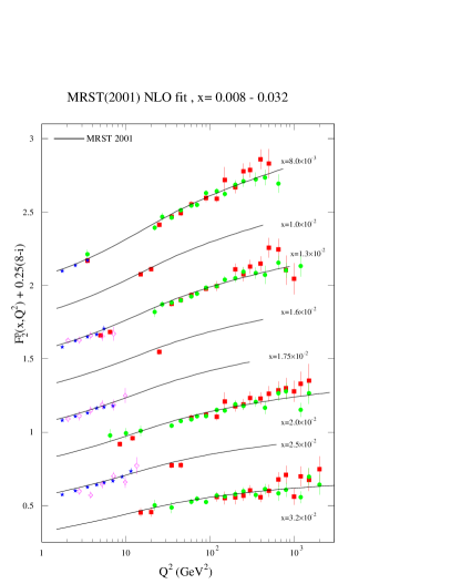
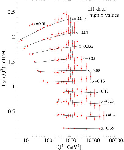
Figure 6: Comparison of MRST(2001) $F_{2}(x,Q^{2})$ with HERA, NMC and E665 data (left) and CTEQ6 $F_{2}(x,Q^{2})$ with H1 data right

Theoretical errors are indicated by some regions where the theory perhaps needs to be improved to fit the data better. There is a reasonably good fit to HERA data, but there are some problems at the highest $Q^{2}$ at moderate $x$, i.e. in $dF_{2}/d\ln Q^{2}$, as seen for MRST and CTEQ in Fig. 6. Also the data require the gluon to be valencelike or negative at small $x$ at low $Q^{2}$, e.g. the ZEUS gluon in Fig. 7, leading to $F_{L}(x,Q^{2})$ being negative at the smallest $x,Q^{2}$ MRST2001 . However, it is not just the low $x$–low $Q^{2}$ data that require this negative gluon. The moderate $x$ data need lots of gluon to get a reasonable $dF_{2}/d\ln Q^{2}$ and the Tevatron jets need a large high $x$ gluon, and this must be compensated for elsewhere. In general MRST find that it is difficult to reconcile the fit to jets and to the rest of the data, and that different data compete over the gluon and $\alpha_{S}(M_{Z}^{2})$. The jet fit is better for CTEQ6 largely due to their different cuts on other data. Other fits do not include the Tevatron jets, but generally produce gluons largely incompatible with this data.

3.2 Types of Theoretical Error, NNLO

It is vital to consider theoretical errors. These include higher orders (NNLO), small $x$ ($\alpha_{s}^{n}\ln^{n-1}(1/x)$), large $x$ ($\alpha_{s}^{n}\ln^{2n-1}(1-x)$) low $Q^{2}$ (higher twist), etc.. Note that renormalization/factorization scale variation is not a reliable method of estimating these theoretical errors because of increasing logs at higher orders, e.g. at small $x$

$$P^{1}_{qg}\sim\alpha_{S}(\mu^{2})\qquad\qquad P^{2}_{qg}\sim\frac{\alpha_{s}(\mu^{2})}{x}\qquad P^{n}_{qg}\sim\frac{\alpha_{S}^{n}(\mu^{2})\ln^{n-2}(1/x)}{x}$$

and scale variations of $P^{1}_{qg},P^{2}_{qg}$ never give an indication of these logs.

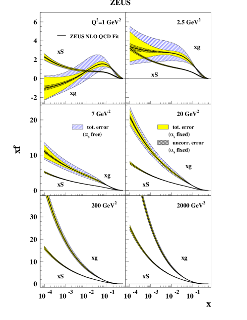
Figure 7: Zeus gluon and sea quark distributions at various $Q^{2}$ values

In order to investigate the true theoretical error we must consider some way of performing correct large and small $x$ resummations, and/or use what we already know about NNLO. The coefficient functions are known at NNLO. Singular limits $x\to 1$, $x\to 0$ are known for NNLO splitting functions as well as limited moments NNLOmoms , and this has allowed approximate NNLO splitting functions to be devised NNLOsplit which have been used in approximate global fits MRSTNNLO . They improve the quality of fit very slightly (mainly at high $x$) and $\alpha_{S}(M_{Z}^{2})$ lowers from $0.119$ to 0.1155. The gluon is smaller at NNLO at low $x$ due to the positive NNLO quark-gluon splitting function. There is also a NNLO fit by Alekhin NNLOAl , with some differences – the gluon is not smaller, probably due to the absence of Tevatron jet data in the fit and to a very different definition of the NNLO charm contribution. There is agreement in the reduction of $\alpha_{S}(M_{Z}^{2})$ at NNLO, i.e. $0.1171\to 0.1143$.

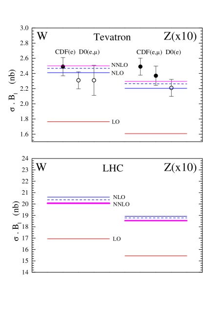
Figure 8: LO, NLO and NNLO predictions for $W$ and $Z$ cross-sections

Using these NNLO partons there is reasonable stability order by order for the (quark-dominated) $W$ and $Z$ cross-sections, as seen in Fig. 8. However, the change from NLO to NNLO is of order $4\%$, which is much bigger than the uncertainty at NLO due to experimental errors. Also, this fairly good convergence is largely guaranteed because the quarks are fit directly to data. There is greater danger in gluon dominated quantities, e.g. $F_{L}(x,Q^{2})$, as shown in Fig. 9. Hence, the convergence from order to order is uncertain.

Figure 9: LO, NLO and NNLO predictions for $F_{L}(x,Q^{2})$

3.3 Empirical approach

We can estimate where theoretical errors may be important by adopting the empirical approach of investigating in detail the effect of cuts on the fit quality, i.e. we try varying the kinematic cuts on data. The procedure is to change $W^{2}_{cut}$, $Q^{2}_{cut}$ and/or $x_{cut}$, re-fit and see if the quality of the fit to the remaining data improves and/or the input parameters change dramatically. (This is similar to a previous suggestion in terms of data sets Collins .) One then continues until the quality of the fit and the partons stabilize cuts .

For $W^{2}_{cut}$ raising from $12.5{\rm GeV}^{2}$ has no effect. When raising $Q^{2}_{cut}$ from $2{\rm GeV}^{2}$ in steps there is a slow, continuous and significant improvement for $Q^{2}$ up to $>12{\rm GeV}^{2}$ (631 data points cut) – suggesting that any corrections are probably higher orders not higher twist. The input gluon becomes slightly smaller at low $x$ at each step (where one loses some of the lowest $x$ data), and larger at high $x$. $\alpha_{S}(M_{Z}^{2})$ slowly decreases by about $0.0015$. The fit improves for Tevatron jets and BCDMS data. Raising $x_{cut}$ leads to continuous improvement with stability reached at $x=0.005$ (271 data points cut) with $\alpha_{S}(M_{Z}^{2})\to 0.118$. There is an improvement in the fit to HERA, NMC and Tevatron jet data, and much reduced tension between the data sets. At each step the moderate $x$ gluon becomes more positive, at the expense of the gluon below the cut becoming very negative and $dF_{2}(x,Q^{2})/d\ln Q^{2}$ being incorrect. However, higher orders could cure this in a quite plausible manner, e.g. adding higher order terms to the splitting functions

$$P_{gg}\to....+\frac{3.6\bar{\alpha}_{S}^{4}}{x}\biggr{(}\frac{\ln^{3}(1/x)}{6}-\frac{\ln^{2}(1/x)}{2}\biggr{)},$$

$$P_{qg}\to....+\frac{4.3N_{f}\bar{\alpha}_{S}^{5}}{6x}\biggr{(}\frac{\ln^{3}(1/x)}{6}-\frac{\ln^{2}(1/x)}{2}\biggr{)},$$

leaves the fit above $x=0.005$ largely unchanged, but solves the problem below $x=0.005$. (Saturation corrections seem to make the fit worse.) Hence, the cuts are suggestive of theoretical errors for small $x$ and/or small $Q^{2}$. Predictions for $W$ and Higgs cross-sections at the Tevatron are still safe if $x_{cut}=0.005$, since they do not sample partons at lower $x$, and change in a smooth manner as $x_{cut}$ is lowered, due to the altered partons above $x_{cut}$, outside the limits set by experimental errors, as seen in Fig. 6.

4 Conclusions

One can perform global fits to all up-to-date data over a wide range of parameter space, and there are various ways of looking at uncertainties due to errors on data alone. There is no totally preferred approach. The errors from this source are rather small – $\sim 1-5\%$ except in a few regions of parameter space and are similar using various approaches. The uncertainty from input assumptions e.g. cuts on data, parameterizations etc., are comparable and sometimes larger, which means one cannot believe one group’s errors.

The quality of the fit is fairly good, but there are some slight problems. These imply that errors from higher orders/resummation are potentially large in some regions of parameter space, and due to correlations between partons these affect all regions (the small $x$ gluon influences the large $x$ gluon). Cutting out low $x$ and/or $Q^{2}$ data allows a much-improved fit to the remaining data, and altered partons. Hence, for some processes theory is probably the dominant source of uncertainty at present and a systematic study is a priority.

References

- (1) A.D. Martin et al., Eur. Phys. J. C23 73 (2002).
- (2) CTEQ Collaboration: J. Pumplin et al., JHEP 0207:012 (2002).
- (3) M. Botje, Eur. Phys. J. C14 285 (2000).
- (4) W.T. Giele and S. Keller, Phys. Rev. D58 094023 (1998); W.T. Giele, S. Keller and D.A. Kosower, hep-ph/0104052.
- (5) S.I. Alekhin, Phys. Rev. D63 094022 (2001).
- (6) H1 Collaboration: C. Adloff et al., Eur. Phys. J. C21 33 (2001).
- (7) A.M. Cooper-Sarkar, hep-ph/0205153, J. Phys. G28 2669 (2002); ZEUS Collaboration: S. Chekanov et al., hep-ph/0208023.
- (8) H1 Collaboration: C. Adloff et al., Eur. Phys. J. C13 609 (2000); H1 Collaboration: C. Adloff et al., Eur. Phys. J. C19 269 (2001).
- (9) ZEUS Collaboration: S. Chekanov et al., Eur. Phys. J. C21 443 (2001); ZEUS Collaboration: S. Chekanov et al., hep-ph/0208040.
- (10) M.R. Adams et al., Phys. Rev. D54 3006 (1996).
- (11) BCDMS Collaboration: A.C. Benvenuti et al., Phys. Lett. B223 485 (1989); BCDMS Collaboration: A.C. Benvenuti et al., Phys. Lett. B236 592 (1989).
- (12) L.W. Whitlow et al., Phys. Lett. B282 475 (1992), L.W. Whitlow, preprint SLAC-357 (1990).
- (13) NMC Collaboration: M. Arneodo et al., Nucl. Phys. B483 3 (1997); Nucl. Phys. B487 3 (1997).
- (14) CCFR Collaboration: U.K. Yang et al., Phys. Rev. Lett. 86 2742 (2001); CCFR Collaboration: W.G. Seligman et al., Phys. Rev. Lett. 79 1213 (1997).
- (15) ZEUS Collaboration: J. Breitweg et al., Eur. Phys. J. C12 35 (2000).
- (16) H1 Collaboration: C. Adloff et al., Phys. Lett. B528 1999 (2002);
- (17) E605 Collaboration: G. Moreno et al., Phys. Rev. D43 2815 (1991).
- (18) E866 Collaboration: R.S. Towell et al., Phys. Rev. D64 052002 (2001).
- (19) CDF Collaboration: F. Abe et al., Phys. Rev. Lett. 81 5744 (1998).
- (20) D0 Collaboration: B. Abbott et al., Phys. Rev. Lett. 86 1707 (2001).
- (21) CDF Collaboration: T. Affolder et al., Phys. Rev. D64 032001 (2001).
- (22) NuTeV Collaboration: M. Goncharov et al., hep-ex/0102049.
- (23) CTEQ Collaboration: D. Stump et al., Phys. Rev. D65 014012 (2002).
- (24) CTEQ Collaboration: J. Pumplin et al., Phys. Rev. D65 014011 (2002).
- (25) CTEQ Collaboration: J. Pumplin et al., Phys. Rev. D65 014013 (2002).
- (26) A.D.Martin et al hep-ph/0211080.
- (27) R.S. Thorne et al., hep-ph/0205233, J. Phys. G28 2717 (2002).
- (28) C. Pascaud and F. Zomer 1995 Preprint LAL-95-05.
- (29) S.A. Larin et al., Nucl. Phys. B492 338 (1997); A. Rétey and J.A.M. Vermaseren, Nucl. Phys. B604 281 (2001).
- (30) W.L. van Neerven and A. Vogt, Phys. Lett. B490 111 (2000).
- (31) A.D. Martin et al., Phys. Lett. B531 216 (2002).
- (32) S.I. Alekhin, Phys. Lett. B519 57 (2001).
- (33) J. C. Collins and J. Pumplin, hep-ph/0105207.
- (34) A.D. Martin, R.G. Roberts, W.J. Stirling and R.S. Thorne, in preparation.