CERN-TH/2002-285 IFT - 20/2002 hep-ph/0211112 September 2002 Longitudinal virtual photons and the interference terms in $ep$ collisions

Abstract

The importance of the contributions of the longitudinally polarized virtual photon $\gamma^{\ast}_{L}$ in $ep$ collisions is investigated. We derive the factorization formulae for the unpolarized inclusive and semi-inclusive $ep$ collisions in an arbitrary reference frame. The numerical calculations for the large-$p_{T}$ (prompt) photons production in the unpolarized Compton process $ep\rightarrow e\gamma X$ at the $ep$ HERA collider are performed in the Born approximation. We studied various distributions in the $ep$ centre-of-mass frame and found that the differential cross section for the longitudinally polarized intermediate photon, $d\sigma_{L}$, and the term due to the interference between the longitudinal- and transverse-polarization states of the photon, $d\tau_{LT}$, are small, i.e. below $10\%$ of the cross section. Moreover, these two contributions almost cancel one another, leading to a stronger domination of the transversely polarized virtual photon, even for its large virtuality $Q^{2}$. Relevance of the resolved longitudinal photon in a jet production in DIS events at HERA is commented. A relatively large ($\sim 30\%$) effect due to the interference term $d\tau_{LT}$ was found in the azimuthal-angle distribution in the Breit frame.

1 Introduction

Assuming that the one-photon exchange dominates in the deep inelastic lepton–nucleon collisions (DIS), a cross section for such a process can be described in terms of two transverse (T) and one longitudinal (L) polarization states of the intermediate virtual photon $\gamma^{\ast}$. The differential cross section for the unpolarized $lN\rightarrow lX$ process can always be decomposed into two differential cross sections, $d\sigma_{T}$ and $d\sigma_{L}$, describing the processes with the transversely and the longitudinally polarized $\gamma^{\ast}$, $\gamma^{\ast}_{T}N\rightarrow X$ and $\gamma^{\ast}_{L}N\rightarrow X$, respectively [1]–[6]. When the initial particles in the discussed process $lN\rightarrow lX$ are polarized, or when for the unpolarized particles a semi-inclusive process $lN\rightarrow laX$ is considered, there appear in addition terms coming from the interference between the longitudinally and transversely polarized virtual photons, and between two different transverse-polarization states of $\gamma^{\ast}_{T}$, $d\tau_{LT}$ and $d\tau_{TT}$, respectively [6].

It is well known that for the two-photon exchange processes, for instance in the $e^{+}e^{-}$ collisions, the interference terms occur in the cross sections, as discussed in [6, 9]. The detailed study of relevance of various contributions, especially of the interference terms, has been performed in [10, 11] for the process $e^{+}e^{-}\rightarrow e^{+}e^{-}\mu^{+}\mu^{-}$, for the kinematical range of the PLUTO and LEP experiments. For a corresponding subprocess $\gamma^{\ast}\gamma^{\ast}\rightarrow\mu^{+}\mu^{-}$ large cross sections for the contribution involving at least one longitudinally polarized photon were found. Moreover, the interference terms were found to give a large negative contribution. Both contributions vary strongly as a function of the kinematical variables, and for some kinematical regions a cancellation between the cross sections for processes with one or two $\gamma_{L}^{\ast}$ and the interference contributions occurs. The conclusion from this analysis was that both types of contributions have to be taken into account in extracting from the data the leptonic (mionic) structure functions of the virtual photon (see also [12]). However, in some of the measurements of the structure functions $F_{2}^{\gamma^{\ast}}$ and $F_{L}^{\gamma^{\ast}}$, the interference terms and cross section for two longitudinally polarized virtual photons were neglected, see [13, 14], and [15].

The contributions due to the longitudinally polarized virtual photons occur also in electroproduction and the question is how significant such contributions are. Moreover, this question is related to the ongoing discussion on the relevance of the resolved-$\gamma^{\ast}_{L}$ contributions in the hard processes [16]–[22]. For example, it was pointed out in [22] that, in the case of the dijet production in the $ep$ HERA collider, the contributions coming from the longitudinally polarized photon are sizeable and the partonic content of the $\gamma^{\ast}_{L}$ should be taken into account in describing the data. However, it is clear that the study of cross sections with $\gamma^{\ast}_{L}$ for the large-$p_{T}$ processes should be accompanied by a consideration of the corresponding interference terms containing $\gamma^{\ast}_{L}$. Unfortunately, there is a lack of such studies in the literature. In this paper we would like to initiate a discussion on the relevance of such terms in the semi-inclusive $ep$ processes.

It is well known that to get access to the interference between $\gamma^{\ast}_{L}$ and $\gamma^{\ast}_{T}$, or between two different transverse-polarization states of $\gamma^{\ast}$, it is natural to consider the azimuthal-angle dependence in a special reference frame called the Breit frame [28]–[35]. Recently, the azimuthal asymmetries for the charged-hadrons production in the neutral-current deep inelastic $e^{+}p$ scattering have been measured with the ZEUS detector at HERA [41], and indeed effects due to the corresponding interference terms were observed.

In this article we study the contributions due to $\gamma^{\ast}_{L}$ and $\gamma^{\ast}_{T}$ in unpolarized $ep$ collisions at HERA, taking as an example the process with a production of high-$p_{T}$ (prompt) photon: $ep\rightarrow e\gamma X$ (Compton process). In Section 2 a short derivation of the factorization formulae for the inclusive and semi-inclusive $ep$ processes is presented in an arbitrary frame (some details are given also in Appendix A). In the case of the semi-inclusive collision, two cross sections, $d\sigma_{T}$ and $d\sigma_{L}$, and two additional terms due to the interference between different polarization states of $\gamma^{\ast}$, $d\tau_{LT}$ and $d\tau_{TT}$, appear. The relation of these interference terms to the contributions proportional to $\cos\phi$ and $\cos 2\phi$ in the azimuthal-angle distribution for a final $\gamma$ in the Breit frame is discussed in Section 3 and Appendix B. Section 4 is devoted to the numerical studies of the different contributions for the process $ep\rightarrow e\gamma X$ in the Born approximation. Conclusions are presented in Section 5. In the Appendices the explicit form of the polarization vectors of the $\gamma^{\ast}$ and factorization formulae for the semi-inclusive process are presented both in a frame-independent form and for the Breit frame.

2 Factorization in the inclusive and semi-inclusive
unpolarized lepton–nucleon scattering

2.1 Inclusive process $ep\rightarrow eX$ (DIS)

We start with a short description of the standard DIS process for unpolarized $ep$ collisions (Fig. 1),

$$ep\rightarrow eX\;,$$ (1)

assuming that the one-photon exchange dominates. The corresponding differential cross section is denoted by $d\sigma^{ep\rightarrow eX}$, and we use the following notation for the kinematical variables: $k^{\mu}$ ($k^{\prime\;\mu}$) denotes the four-momentum of the initial (final) electron, $p_{p}^{\mu}$ the four-momentum of the initial proton, $q^{\mu}$ the four-momentum of the intermediate photon, and $Q^{2}=-q^{2}>0$ is the photon’s virtuality. We denote by $\varepsilon^{\mu}_{i}$ ($i=T_{1},T_{2},L$) the two transverse- and one longitudinal-polarization vectors of the exchanged virtual photon $\gamma^{\ast}$. The standard scaling variables are $x=Q^{2}/2p_{p}q$ and $y\;=\;p_{p}q/p_{p}k$.

Figure 1: Kinematics and notation for the process $ep\rightarrow eX$ with the one-photon exchange. The optical theorem relation of the squared matrix element for $ep\rightarrow eX$ and the imaginary part of the amplitude for $ep\rightarrow ep$ at $t=0$.

It is well known that for the considered process (1) there is a factorization of the differential cross section onto the lepton and hadron parts and a separation between the contributions of the longitudinal- and transverse-polarization states of the intermediate photon [1]–[6]. So, we have here:

$$d\sigma^{ep\rightarrow eX}\;=\;\Gamma_{T}\;d\sigma^{\gamma^{\ast}p\rightarrow X}_{T}\;+\;\Gamma_{L}\;d\sigma^{\gamma^{\ast}p\rightarrow X}_{L}\;\equiv\;d\sigma_{T}\;+\;d\sigma_{L}\;,$$ (2)

where $d\sigma^{\gamma^{\ast}p\rightarrow X}_{T}$ and $d\sigma^{\gamma^{\ast}p\rightarrow X}_{L}$ are the cross sections for the $\gamma^{\ast}p$ collision with the virtual photon polarized transversely and longitudinally, respectively. The functions $\Gamma_{T}$ and $\Gamma_{L}$ describe the probabilities of the emission, by the initial electron, of a virtual photon in the transverse- and the longitudinal-polarization states, respectively.

The above factorization and separation formula can be obtained in various ways [1]–[6]. For example, the cross section for the process $ep\rightarrow eX$ (see Fig. 1) can be expressed as a convolution of the lowest order leptonic tensor $L_{e}^{\mu\nu}(k,q)$ and the hadronic tensor $W_{p}^{\mu\nu}(p_{p},q)$, both symmetric in the indices $\mu$ and $\nu$. Namely we have (for $k^{2}=k^{\prime\;2}=0$, $p_{p}^{2}=M^{2}$)

$$d\sigma^{ep\rightarrow eX}\;\sim\;\frac{1}{q^{4}}\;L_{e\;\mu\nu}\;W_{p}^{\mu\nu}\;,$$ (3)

where:

$$L_{e}^{\mu\nu}\;(k,q)\;\;=\;\;2\;(2k^{\mu}k^{\nu}-q^{\mu}k^{\nu}-k^{\mu}q^{\nu}+\frac{1}{2}q^{2}g^{\mu\nu})\;,$$ (4)

$$W_{p}^{\mu\nu}\;(p_{p},q)\;\;=\;\;W_{1}\;(-g^{\mu\nu}+\frac{q^{\mu}q^{\nu}}{q^{2}})\;+\;\frac{W_{2}}{M^{2}}\;(p_{p}^{\mu}-\frac{p_{p}q}{q^{2}}q^{\mu})(p_{p}^{\nu}-\frac{p_{p}q}{q^{2}}q^{\nu})\;.$$ (5)

The gauge invariance leads to the conditions:

$$q_{\mu}L_{e}^{\mu\nu}\;=\;q_{\nu}L_{e}^{\mu\nu}\;=\;0\;,\;\;\;q_{\mu}W_{p}^{\mu\nu}\;=\;q_{\nu}W_{p}^{\mu\nu}\;=\;0\;.$$ (6)

On the other hand, one can express the hadronic tensor in terms of the polarization states of the exchanged photon. Using the explicit form of the longitudinal-polarization vector and the completeness relation given in Appendix A, we obtain

$$W_{p}^{\mu\nu}\;=\;W_{1}\;\sum_{T=T1}^{T2}\;\varepsilon_{T}^{\ast\;\mu}\varepsilon_{T}^{\nu}\;+\;(\bar{W}_{2}-W_{1})\;\varepsilon_{L}^{\ast\;\mu}\varepsilon_{L}^{\nu}\;,\;\;\;\;\;\;\bar{W}_{2}\;=\;\frac{(p_{p}q)^{2}-q^{2}p_{p}^{2}}{-q^{2}}\;\frac{W_{2}}{M^{2}}\;.$$ (7)

From the above form of $W_{p}^{\mu\nu}$ (7) one can easily derive formula (2).

Another way of obtaining the considered formula (2) is “the propagator decomposition method” [26], [27]. In this method the cross section for process (1) is represented in the following form:

$$d\sigma^{ep\rightarrow eX}\;\sim\;L_{e}^{\alpha\beta}\;\frac{g_{\alpha\mu}}{q^{2}}\;\frac{g_{\nu\beta}}{q^{2}}\;W_{p}^{\mu\nu}\;,$$ (8)

where $\frac{g_{\alpha\mu}}{q^{2}}\;\frac{g_{\nu\beta}}{q^{2}}$ represents the propagators of the exchanged photon in the Feynman gauge. One can decompose two propagators occurring in eq. (8) by using the completeness relation (22). This leads straightforwardly to the factorization of the cross section for the considered process and, after some calculations, to the separation into two parts related to $\gamma_{L}^{\ast}$ and $\gamma_{T}^{\ast}$. This method is especially useful in analyzing the semi-inclusive processes, which we will discuss below.

2.2 Semi-inclusive process $ep\rightarrow e\gamma X$ (Compton process)

Let us now consider the semi-inclusive process $ep\rightarrow eaX$, assuming that all particles are unpolarized. Here, in comparison to the DIS process $ep\rightarrow eX$, one additional particle $a$ is produced. In the following we choose as particular final state a prompt photon (i.e. $a=\gamma$), with four-momentum $p$.

We will study the factorization of the cross section for this process, limiting ourselves to the case in which the $\gamma$ is emitted from the hadronic part of the diagram only (Fig. 2). Of course, the final photon can be emitted also from the electron line – a typical bremsstrahlung process also called the Bethe–Heitler process; a relevance of this contribution is discussed at the beginning of Section 4.

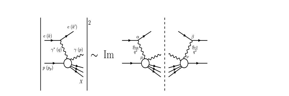
Figure 2: Kinematics and notation for the semi-inclusive process $ep\;\rightarrow\;e\gamma X$ with a one-photon exchange. The optical theorem which relates $\sigma(ep\rightarrow e\gamma X)$ to the imaginary part of the forward amplitude for the process $ep\stackrel{{\scriptstyle\gamma}}{{\longrightarrow}}ep$ $(t=0)$ is also shown.

The differential cross section for the unpolarized process

$$ep\rightarrow e\gamma X\;$$ (9)

can be written as for process (1), namely

$$d\sigma^{ep\rightarrow e\gamma X}\;\sim\;L_{e}^{\alpha\beta}\;\frac{g_{\alpha\mu}}{q^{2}}\;\frac{g_{\nu\beta}}{q^{2}}\;T^{\mu\nu}\;,$$ (10)

where the corresponding hadronic tensor $T^{\mu\nu}(p_{p},q,p)$ is introduced (cf. (8)). Here the hadronic tensor $T^{\mu\nu}(p_{p},q,p)$ depends not only on the four-momenta of the intermediate photon $q$ and of the proton $p_{p}$, but also on the four-momentum of the final photon $p$. New scaling variables appear here, e.g. $z_{\gamma}\;=\;p_{p}p/p_{p}q$. Using “the propagator decomposition method” one can obtain the factorization formula in which the interference between two different transverse-, and between the transverse- and the longitudinal-polarization states of the exchanged photon, denoted by TT and LT (or TL), may appear. We obtain:

$$d\sigma^{ep\rightarrow e\gamma X}\;=\;\sum_{T=T1}^{T2}\;\Gamma_{T}\;d\sigma^{\gamma^{\ast}p\rightarrow\gamma X}_{T}\;+\;\sum_{i,j=T1,T2;i\neq j}\;\Gamma_{ij}\;d\tau^{\gamma^{\ast}p\rightarrow\gamma X}_{ij}\;+\;$$ (11)

$$+\;\Gamma_{L}\;d\sigma^{\gamma^{\ast}p\rightarrow\gamma X}_{L}\;+\;\sum_{T=T1}^{T2}\;(\;\Gamma_{TL}\;d\tau^{\gamma^{\ast}p\rightarrow\gamma X}_{TL}\;+\;\Gamma_{LT}\;d\tau^{\gamma^{\ast}p\rightarrow\gamma X}_{LT}\;)\;.$$ (12)

Below we will use the following short notation for the groups of contributions which appear in (11) and (12):

$$d\sigma^{ep\rightarrow e\gamma X}\;\equiv\;d\sigma_{T}+d\tau_{TT}\;+\;d\sigma_{L}\;+\;d\tau_{LT}.$$ (13)

We see that the cross section (13) for the considered process (9) contains $d\sigma_{T}$, $d\sigma_{L}$ and in addition two interference terms, $d\tau_{TT}$ and $d\tau_{LT}$ (see also [6]). These four terms are related by the optical theorem (see Fig. 2) to the corresponding amplitudes:

$$d\sigma_{T}\;\sim\;\frac{1}{q^{4}}\sum_{T=T1}^{T2}\;[\;(\varepsilon_{T}^{\ast})_{\mu}\;L_{e}^{\mu\nu}\;(\varepsilon_{T})_{\nu}\;]\cdot[\;(\varepsilon_{T})_{\mu}\;T^{\mu\nu}\;(\varepsilon_{T}^{\ast})_{\nu}\;]\;,$$ (14)

$$d\sigma_{L}\;\sim\;\frac{1}{q^{4}}[\;(\varepsilon_{L}^{\ast})_{\mu}\;L_{e}^{\mu\nu}\;(\varepsilon_{L})_{\nu}\;]\cdot[\;(\varepsilon_{L})_{\mu}\;T^{\mu\nu}\;(\varepsilon_{L}^{\ast})_{\nu}\;]\;,$$ (15)

$$d\tau_{TT}\;\sim\;\frac{1}{q^{4}}\sum_{i,j=T1,T2;\;i\neq j}\;[\;(\varepsilon_{i}^{\ast})_{\mu}\;L_{e}^{\mu\nu}\;(\varepsilon_{j})_{\nu}\;]\cdot[\;(\varepsilon_{i})_{\mu}\;T^{\mu\nu}\;(\varepsilon_{j}^{\ast})_{\nu}\;]\;,$$ (16)

$$d\tau_{LT}\;\sim\;\frac{1}{q^{4}}\{\sum_{T=T1,T2}\;[\;(\varepsilon_{L}^{\ast})_{\mu}\;L_{e}^{\mu\nu}\;(\varepsilon_{T})_{\nu}\;]\cdot[\;(\varepsilon_{L})_{\mu}\;T^{\mu\nu}\;(\varepsilon_{T}^{\ast})_{\nu}\;]\;+$$

$$+\;\sum_{T=T_{1},T_{2}}\;[\;(\varepsilon_{T}^{\ast})_{\mu}\;L_{e}^{\mu\nu}\;(\varepsilon_{L})_{\nu}\;]\cdot[\;(\varepsilon_{T})_{\mu}\;T^{\mu\nu}\;(\varepsilon_{L}^{\ast})_{\nu}\;]\;\}.$$ (17)

It is worth noticing that the decomposition of the differential cross section $d\sigma^{ep\rightarrow e\gamma X}$ into three components: $d\hat{\sigma}_{T}=d\sigma_{T}+d\tau_{TT}$, $d\sigma_{L}$ and $d\tau_{LT}$, does not depend on the choice of the reference frame or of the basis for the polarization vectors. Note that in the differential cross section $d\sigma^{ep\rightarrow e\gamma X}$ there are two independent terms related to the longitudinal-polarization state of the virtual photon: $d\sigma_{L}$ and $d\tau_{LT}$.

Obviously the above factorization formula (13) holds for the semi-inclusive process with arbitrary final-state particle $a$.

3 Azimuthal-angle distribution for $ep\rightarrow e\gamma X$

In studies of the process $ep\rightarrow e\gamma X$ it is useful to consider the azimuthal-angle ($\phi$) distribution. This angle is defined as the difference between the azimuthal angle of the final electron ($\phi_{e}$) and that of the final photon $\gamma$ ($\phi_{\gamma}$):

$$\phi\;=\;\phi_{e}\;-\;\phi_{\gamma}\;.$$ (18)

In the special reference frames in which the momenta of the virtual photon and of the proton are antiparallel (for example in the Breit frame or in the $\gamma^{\ast}p$ centre-of-mass frame) $\phi$ is the angle between the electron scattering-plane and the plane defined by the momenta of the exchanged $\gamma^{\ast}$ and the final $\gamma$ (Fig. 3). In such reference frames, the cross section $d\sigma^{ep\rightarrow e\gamma X}/d\phi$ is linear in $\cos\phi$, $\cos 2\phi$, $\sin\phi$ and $\sin 2\phi$. In the Born approximation the terms containing $\sin\phi$ and $\sin 2\phi$ vanish as a consequence of a time-reversal invariance, so the azimuthal-angle distribution reduces to the following form [28]–[35] (see also Appendix B):

$$\frac{d\sigma^{ep\rightarrow e\gamma X}}{d\phi}\;=\;\sigma_{0}\;+\;\sigma_{1}\;\cos\phi\;+\;\sigma_{2}\;\cos 2\phi\;,$$ (19)

with independent on $\phi$ coefficients $\sigma_{0}$, $\sigma_{1}$ and $\sigma_{2}$. These coefficients calculated for instance in the Breit frame, are related to the terms $d\sigma_{T}/d\phi$, $d\sigma_{L}/d\phi$, $d\tau_{LT}/d\phi$ and $d\tau_{TT}/d\phi$, introduced in Sect. 2.2, calculated in the same reference frame. In the circular-polarization basis, where the polarization vectors correspond to the definite helicity states, the term $\sigma_{2}\cos 2\phi$ arises from the interference between two different transverse-polarization states of the exchanged photon ($\sim d\tau_{TT}$). The longitudinal-transverse interference ($\sim d\tau_{LT}$) gives rise to the term $\sigma_{1}\cos\phi$. The $\sigma_{0}$ consists of the sum of the cross sections with the intermediate photon polarized transversely and longitudinally ($\sim(d\sigma_{L}+d\sigma_{T})$). Obviously, since $\sigma_{1}$ and $\sigma_{2}$ (and $\sigma_{0}$) do not depend on $\phi$, the contributions due to the interferences will disappear after integrating over $\phi$.

The interference terms can be extracted in a straightforward way from the data for the azimuthal-angle distribution $d\sigma/d\phi$ in the frames with antiparallel virtual photon’s and proton’s momenta, for example in the Breit frame.

Figure 3: The azimuthal angle $\phi$ defined in the Breit frame for the Compton process $ep\rightarrow e\gamma X$.

In other frames, i.e. in frames in which the momenta of the virtual photon and proton are not antiparallel, the dependence on the azimuthal angle is more complicated. Each of the four terms contributing to the differential cross section (see eqs. (13)–(17)) consists of the part that does not depend on the azimuthal angle. Consequently the interference terms integrated over a $\phi$ give non-zero result. This important fact was mentioned in papers [7, 8], where the Higgs boson production via $WW$ or $ZZ$ fusion in $e^{+}e^{-}$ collisions has been studied.

4 Numerical results

We perform calculations of the cross sections for the unpolarized Compton process $ep\rightarrow e\gamma X$. We consider the one-photon exchange only; this approximation is correct for the virtuality of the intermediate photon $Q^{2}\ll M_{Z}^{2}$, while for larger values of $Q^{2}$ the $Z/W$ boson exchange should be included. Below we present predictions for HERA for the beam energies equal to: $E_{e}=27.5$ GeV and $E_{p}=920$ GeV.

We analyze, at the Born level, the emission of the prompt photon from the hadronic vertex, i.e. we consider the Compton subprocess: $\gamma^{\ast}q\rightarrow\gamma q$. In principle, the Bethe–Heitler (BH) process, where the prompt photons can be emitted from the electron line and the interference between the Compton and BH amplitudes, should also be included in the calculation [37, 38, 39]. Both latter contributions dominate the cross section in the electron–proton centre-of-mass frame for the rapidity range of the final photon’s $Y<0$, while for greater rapidities the Compton process dominates [40]. We expect that our results should be reliable for positive values of the Y in the $CM_{ep}$.

Results presented below were obtained for two frames: the electron–proton centre-of-mass frame ($CM_{ep}$) and the Breit frame. The transverse momentum $p_{T}$ of the final photon is defined as perpendicular to the direction of the $ep$ collision in the $CM_{ep}$ frame or to the direction of the $\gamma^{\ast}p$ collision in the Breit frame.

For the quark density in the proton $q^{p}(x,\tilde{Q}^{2})$ we use the CTEQ5L parton parametrization [36] with a fixed number of flavours: $N_{f}=4$. This parametrization imposes the limit on a range of a hard scale $\tilde{Q}^{2}$: it has to be greater than $1$ GeV and less than $10^{4}$ GeV. In our calculations we use as a hard scale $\tilde{Q}$ the transverse momentum of the final photon $p_{T}$; effects of other choices of the hard scale were studied by us, and are briefly discussed below.

Figure 4: Various contributions to the differential cross section $d\sigma/dQ^{2}$ in the $CM_{ep}$ frame for the prompt-photon production ($(p_{T})_{min}=$ 1  GeV) at HERA. The contribution due to the transverse-polarization states: $d\hat{\sigma}_{T}=d\sigma_{T}+d\tau_{TT}$ (long-dashed line), the cross section for the longitudinally polarized intermediate photon: $d\sigma_{L}$ (short-dashed line) and the absolute value of the interference term: $|d\tau_{LT}|$ (dotted line), together with the sum of all terms $d\sigma$ (solid line), are shown.

First we consider the differential cross section $d\sigma/dQ^{2}$ in the $CM_{ep}$ frame, integrated over $p_{T}$ from $(p_{T})_{min}=1$ GeV to $(p_{T})_{max}=\sqrt{S_{ep}}/2$, as a function of $Q^{2}$. We consider separately four frame-independent contributions: $d\hat{\sigma}_{T}=d\sigma_{T}+d\tau_{TT}$, $d\sigma_{L}$ and $|d\tau_{LT}|$ as a function of $Q^{2}$. As it is presented in Fig. 4, the $Q^{2}$ dependence is roughly similar for all contributions. The differential cross section is dominated by the contribution due to the transversely polarized intermediate photon, i.e. $d\hat{\sigma}_{T}=d\sigma_{T}+d\tau_{TT}$. The $d\sigma_{L}$ contributes at the few per cent level to the whole cross section, similarly to the interference term $d\tau_{LT}$. Moreover, $d\sigma_{L}$ is positive while $d\tau_{LT}$ negative, and these two contributions almost cancel one another. The resulting cross section $d\sigma/dQ^{2}$, even for large values of $Q^{2}$ ($\sim 100$ GeV²), is described with a high accuracy by the $d\hat{\sigma}_{T}$ term only.

Figure 5: The ratio $[d\sigma_{L}/dQ^{2}]\;/\;[d\sigma_{T}/dQ^{2}]$ for prompt-photon production in the $ep$ collision at HERA ($(p_{T})_{min}=$ 1 GeV), as a function of $Q^{2}$, in the $CM_{ep}$ frame (solid line) and in the Breit frame (dashed line), is shown.

The ratio $[d\sigma_{L}/dQ^{2}]\;/\;[d\sigma_{T}/dQ^{2}]$ as a function of virtuality $Q^{2}$ for the $CM_{ep}$ frame and the Breit frame is presented in Fig. 5. In the $CM_{ep}$ frame it grows slowly with the virtuality of the intermediate photon up to $Q^{2}\sim(p_{T})_{min}^{2}$, then this ratio slowly decreases. In the Breit frame the corresponding growth is much faster, the ratio reaches its maximum at much larger $Q^{2}$ (10 times $(p_{T})_{min}$). Also the maximum is higher (two times) in the Breit frame than in the $CM_{ep}$ one. At $Q^{2}=100$ GeV² the considered ratio $[d\sigma_{L}/dQ^{2}]\;/\;[d\sigma_{T}/dQ^{2}]$ is equal to about $0.02$ for the $CM_{ep}$ frame, while it is about four times larger for the Breit frame.

Figure 6: Various contributions to the $d\sigma/(dYdp_{T}$) in the $CM_{ep}$ frame for high-$p_{T}$ photon production at HERA ($(p_{T})_{min}=$ 1 GeV) as a function of a) $p_{T}$ at $Y=0$ and b) $Y$ at $p_{T}=5$  GeV. Same notation as in Fig. 4.

Figure 6 shows results for the differential cross section $d\sigma/dYdp_{T}$ in the $CM_{ep}$ frame. The $p_{T}$ distribution for a fixed value of the photon rapidity, $Y=0$, is shown in Fig. 6 (left), while the $Y$ distribution at $p_{T}=5$ GeV is shown in Fig. 6 (right). We see that these distributions are described with a very good accuracy by the $d\hat{\sigma}_{T}$ terms only. Contributions $d\sigma_{L}$ and $d\tau_{LT}$ are small and there is almost a cancelation between them. In other words, the measurements of such cross sections in the $CM_{ep}$ frame are not sensitive to the individual contributions involving the longitudinally polarized virtual photon: $d\sigma_{L}$ and/or $d\tau_{LT}$.

Another interesting and important fact is that, in the $CM_{ep}$ frame the interference term gives non-vanishing contributions even for the cross sections integrated over the azimuthal angle (defined by eq.(18)), as it was supposed. This can be seen in the azimuthal-angle distribution for the interference term in this frame (Fig. 7). It is clear that the $d\tau_{LT}$ integrated over $\phi$ gives a non-vanishing contribution. This is the main difference between the $CM_{ep}$ frame and the Breit frame (or other frames with antiparallel virtual photon and proton). In the latter frame the contributions due to the interference terms disappear in the cross sections integrated over $\phi$, see below.

Figure 7: The $d\hat{\sigma}_{T}=d\sigma_{T}+d\tau_{TT}$, $d\sigma_{L}$ and $d\tau_{LT}$ contributions to the high-$p_{T}$ photon production at HERA. Results for the azimuthal-angle distributions $d\sigma/(dYdp_{T}\;d\phi)$ in the $CM_{ep}$ frame, for $Y=0$ and $p_{T}=5$ GeV.

Finally, we study the azimuthal-angle distribution of the final photon in the Breit frame (19). As discussed in Sect. 3, in this frame the coefficients $\sigma_{1}$, $\sigma_{2}$ and $\sigma_{0}$ are independent of $\phi$. They are directly related to the interference terms $d\tau_{TT}/d\phi$, $d\tau_{LT}/d\phi$ and to the sum: $d\sigma_{L}/d\phi+d\sigma_{T}/d\phi$, respectively. (For more details see also Appendix B).

The numerical calculations for the azimuthal-angle distribution for the Compton process in the Breit frame are performed for the same kinematical region in which the charged-hadrons production was measured in the ZEUS experiment at the HERA collider [41]: $180$ GeV${}^{2}<Q^{2}<7220$ GeV², $0.2<y<0.8$, $0.2<z_{\gamma}<1.0$ and the $(p_{T})_{min}=2$ GeV. Results for the Compton process are presented in Fig. 8. The contribution related to the interference between two transverse polarization states of $\gamma^{\ast}$ (the term proportional to $\sigma_{2}\cos 2\phi$) gives a negligible effect, while the interference between the virtual photon polarized longitudinally and transversely (the term proportional to $\sigma_{1}\cos\phi$) leads to a visible effect (about $30\%$). Clearly, both interference contributions being symmetric under the $\phi\rightarrow-\phi$ transformation disappear after the integration over the $\phi$ angle over $-\pi$ to +$\pi$.

Figure 8: The $\phi$ distributions in the Breit frame (see text) obtained for: $180$ GeV${}^{2}<Q^{2}<7220$ GeV², $0.2<y<0.8$, $0.2<z_{\gamma}<1.0$ and the $(p_{T})_{min}=2$ GeV, for $ep\rightarrow e\gamma X$ at HERA.

Now we compare our results for the prompt-photon production with those obtained in the ZEUS experiment for the charged hadrons [41]. In the ZEUS data the term $\sigma_{1}\cos\phi$ is clearly seen for all four considered values of $p_{T}$ cut: $(p_{T})_{min}\;=\;0.5$, $1$, $1.5$ and $2$ GeV, while the term $\sigma_{2}\cos 2\phi$ gives a negligible effect for lower values of $(p_{T})_{min}$, becoming visible for a larger $(p_{T})_{min}$. This is different from the Compton process discussed above, where the corresponding $\sigma_{2}$ term is very small, even for $(p_{T})_{min}=2$ GeV (see Fig. 8). This difference arises from the following fact: in the case of the Compton process $ep\rightarrow e\gamma X$, calculated in the Born approximation, there is only one subprocess $\gamma^{\ast}q\rightarrow\gamma q$ that contributes to the cross section. For the charged-hadrons production there are, at the Born level, two subprocesses, $\gamma^{\ast}q\rightarrow gq$ and $\gamma^{\ast}g\rightarrow q\bar{q}$. The second process $\gamma^{\ast}g\rightarrow q\bar{q}$ dominates in the $\sigma_{2}\cos 2\phi$ term, while the contribution coming from the process $\gamma^{\ast}q\rightarrow gq$ (analogous to our $\gamma^{\ast}q\rightarrow\gamma q$ process) dominates in the $\sigma_{1}\cos\phi$ term. Therefore both contributions can (and are) visible in the azimuthal-angle distribution of the charged-hadrons production, while in our case, based on one subprocess, the visible effect is expected only in $\sigma_{1}\cos\phi$.

Finally, let us comment on the dependence of our results on a choice of the hard scale. Although all the cross sections presented above are computed for a hard scale equal to $p_{T}$, one can choose for the considered process also other scales: e.g. $Q^{2}$ or $\sqrt{p_{T}^{2}+Q^{2}}$. We have checked by an explicit calculation that the cross sections obtained when the hard scale is equal to $Q^{2}$ or $\sqrt{p_{T}^{2}+Q^{2}}$ are slightly larger (not more than 5%) than the ones obtained when the hard scale is equal to $p_{T}$. This difference is not significant and does not change our main conclusions.

5 Conclusions

In this paper we investigated the importance of the contributions due to the longitudinal virtual photon in unpolarized, semi-inclusive $ep$ collisions at HERA. In general there are two such contributions: the cross section for $\gamma_{L}^{\ast}p$ collision $d\sigma_{L}$, and the interference term $d\tau_{LT}$. As a particular semi-inclusive process we chose the Compton process, where the prompt photon is emitted from the hadronic system. For the semi-inclusive process $ep\rightarrow e\gamma X$ at HERA energies we analyzed three frame-independent contributions: the cross section $d\sigma_{L}$, $d\tau_{LT}$ coming from the interference between the longitudinal- and the transverse-polarization states of $\gamma^{\ast}$ and the contribution due to $\gamma^{\ast}_{T}$: $d\hat{\sigma}_{T}=d\sigma_{T}+d\tau_{TT}$. The calculations were performed in the Born approximation. In the $ep$ centre-of-mass frame we studied various distributions, the $p_{T}$ and the rapidity distributions, as well as the $Q^{2}$ distribution, were the the contributions mentioned simply add up. We found that both $d\sigma_{L}$ and $d\tau_{LT}$ are small and of similar size, below $10\%$ of the cross section. This suggests that the contribution $d\sigma_{L}$ and the interference terms need be included on the same footing. Additionally, because of their opposite signs, they almost cancel in the cross section. This leads to a strong domination of the considered cross section by a contribution due to transversely polarized virtual photon, even for large values of its virtuality.

Although our results are based on the Compton process in a Born approximation only, we think that they already shed some light on the importance of contributions due to $\gamma_{L}^{\ast}$ in other semi-inclusive processes, like the jet production in the DIS events at the HERA collider. It is clear that in order to reach a final conclusion on the importance of the contributions related to the $\gamma_{L}^{\ast}$, as advocated in some analyses, further studies are needed, with the incorporation of the relevant interference terms for consistency.

The studies of the azimuthal-angle dependence of $d\sigma^{ep\rightarrow e\gamma X}/d\phi$ in the Breit frame give access to the interference term $d\tau_{LT}$, as expected. Its effect is about $30\%$, showing in this case the importance of the $\gamma_{L}^{\ast}$ contributions in the form of the interference $d\tau_{TL}$ term.

Acknowledgements  

We would like to acknowledge I.F. Ginzburg, P.M. Zerwas, P.J. Mulders, S. Brodsky, L. Levchuk, and A. Szczurek for interesting and fruitful discussions.

This research has been partly supported by the Polish Committee for Scientific Research, Grant No 2P03B05119(2000-2002) and by the European Community’s Human Potential Program under Contract HPRN-CT-2000-00149 Physics in Collision.

Appendix

Appendix A. Polarization vectors of $\gamma^{\ast}$ and factorization formula for the Compton process  

Below we present the polarization vectors of a virtual photon $\gamma^{\ast}$ (with the four-momentum $q^{\mu}$: $q^{2}<0$) in a form that is independent of the reference frame for the two types of basis for the polarization vectors: linear and circular.

A.1 Polarization vectors

The Lorentz condition for the polarization vectors gives rise to the physical observables

$$\varepsilon_{\mu}\;q^{\mu}\;\;=\;\;0\;.$$ (20)

Consequently, the scalar-polarization state of the $\gamma^{\ast}$, described by the following vector

$$\varepsilon^{\mu}_{S}\;\;=\;\;\frac{q^{\mu}}{\sqrt{-q^{2}}}\;,$$ (21)

does not contribute to the physical observables. We can write the completeness relation as follows:

$$-\;g^{\mu\nu}\;+\;\frac{q^{\mu}q^{\nu}}{q^{2}}\;\;=\;\;\sum_{T=T1}^{T2}\;(\varepsilon^{\ast}_{T})^{\mu}\;(\varepsilon_{T})^{\nu}\;-\;(\varepsilon^{\ast}_{L})^{\mu}\;(\varepsilon_{L})^{\nu}\;.$$ (22)

The four polarization vectors of the virtual photon satisfy also the orthonormality relation:

$$(\varepsilon^{\ast}_{m})_{\mu}\;(\varepsilon_{n})^{\mu}\;\;=\;\;\zeta_{m}\delta_{mn}\;,\;\;\;\;\;\;\mbox{where}\;\;\;\zeta_{L}=1\;,\;\;\;\zeta_{S}=\zeta_{T}=-1\;.$$ (23)

A.2 Linear polarization

The linear-polarization states are represented by the real polarization vectors. The longitudinal-polarization vector ($\varepsilon^{2}_{L}=1$) for the electron–proton collisions depends on the four-momenta of the virtual photon ($q^{\mu}$) and proton ($p_{p}^{\mu}$) or quark ($p_{q}^{\mu}=xp_{p}^{\mu}$), (see also [6]):

$$\varepsilon^{\mu}_{L}\;\;=\;\;\frac{(p_{p}q)q^{\mu}-q^{2}p_{p}^{\mu}}{\sqrt{-q^{2}}\;(p_{p}q)}\;.$$ (24)

For the semi-inclusive processes we need to construct the two transverse-polarization vectors ($\varepsilon^{2}_{T}=-1$). In order to construct them we have to introduce the third four-momentum; for the Compton process we use the momentum of the final photon ($p^{\mu}$) and obtain:

$$\varepsilon^{\mu}_{1}\;\;=\;\;\frac{-2}{\sqrt{stu}}\;[\;(p_{p}p)q^{\mu}-(p_{p}q)p^{\mu}+\frac{(qp)(p_{p}q)-q^{2}(p_{p}p)}{(p_{p}q)}\;p_{p}^{\mu}\;]$$ (25)

and

$$\varepsilon^{\mu}_{2}\;\;=\;\;\frac{2}{\sqrt{stu}}\;\epsilon^{\mu\nu\alpha\beta}\;q_{\nu}(p_{p})_{\alpha}p_{\beta},$$ (26)

where $stu=4[2(p_{p}q)(p_{p}p)(qp)-q^{2}(p_{p}p)^{2}]$ .
This transverse-polarization vectors satisfy in addition the following equations:

$$\varepsilon_{1}p_{p}=0,\;\;\;\;\varepsilon_{1}p=0\;\;\;\;{\rm and}\;\;\;\;\varepsilon_{2}p_{p}=0.$$

A.3 Circular polarization

Using the above forms of the linear-polarization vectors (eqs. (24), (25), (26)), one can define the circular-polarization vectors of the $\gamma^{\ast}$, namely the longitudinal-polarization vector denoted by $\varepsilon^{\mu}_{0}$ and the transverse ones denoted by $\varepsilon^{\mu}_{+}$ and $\varepsilon^{\mu}_{-}$. These vectors correspond to the helicities of the intermediate photon equal to $\lambda=0,+,$ and $-$, respectively. We get

$$\varepsilon^{\mu}_{0}\;\;=\;\;i\;\varepsilon^{\mu}_{L},$$ (27)

$$\varepsilon^{\mu}_{+}\;\;=\;\;\frac{1}{\sqrt{2}}\;(\;\varepsilon^{\mu}_{1}\;+\;i\varepsilon^{\mu}_{2}\;),$$ (28)

and

$$\varepsilon^{\mu}_{-}\;\;=\;\;\frac{1}{\sqrt{2}}\;(\;\varepsilon^{\mu}_{1}\;-\;i\varepsilon^{\mu}_{2}\;).$$ (29)

A.4 Factorization formula for the Compton process

The general factorization formula for the electron–quark scattering with the photon in the final state has the following form for massless quarks:

$$d\sigma^{eq\rightarrow eq\gamma}\;\sim\;e^{6}Q_{q}^{4}\;{\rm Re}\;[L_{e\;\alpha\beta}\frac{g^{\alpha\mu}g^{\nu\beta}}{Q^{4}}T_{\mu\nu}]\;=\;\frac{e^{6}Q_{q}^{4}}{Q^{4}}\;{\rm Re}\;[\sum_{i,j}\;\zeta_{ij}\;\underbrace{(L_{e\;\alpha\beta}\varepsilon_{i}^{\ast\alpha}\varepsilon_{j}^{\beta})}_{\equiv\;L_{ij}}\;\underbrace{(\varepsilon_{j}^{\ast\nu}\varepsilon_{i}^{\mu}T_{\mu\nu})}_{\equiv\;T_{ji}}]\;,$$ (30)

where $i,j$ denote the polarization states of the virtual photon ($i,j=L,T1,T2$ for the linear polarization and $i,j=0,+,-$ for the circular polarization), $\zeta_{LT}=\zeta_{TL}=-1$, while in the remaining cases $\zeta_{ij}=1$. The tensor $L_{e\;\mu\nu}(q,k)$ is related to the emission of the virtual photon by the electron, while the tensor $T_{\mu\nu}(q,p_{q},p)$ describes the absorption of the virtual photon by the quark (from proton), with the subsequent production of a prompt photon.

Two of the contributions to the cross section, $d\sigma_{T}$ (14) and $d\tau_{TT}$ (16), depend on the choice of the basis of the polarization states of $\gamma^{\ast}$. But the propagator decomposition method assures that their sum: $d\hat{\sigma}_{T}=d\sigma_{T}+d\tau_{TT}$, as well as the individual terms $d\sigma_{L}$ (15) and $d\tau_{LT}$ (17) are the same in any basis. This fact can also be checked by using the relations between the linear and circular transverse-polarization vectors (eqs. (28), (29)).

The calculations presented in this paper rely on the lowest order subprocess $\gamma^{\ast}q\;\rightarrow\;\gamma q$ (the Born approximation). The corresponding partonic tensor has the following form:

$$T^{\mu\nu}(q,p_{q},p)\;\;=\;\;\frac{2}{su}\;\{\;g^{\mu\nu}(u^{2}+s^{2}+2q^{2}t)\;+\;2u[2q^{\mu}q^{\nu}+q^{\mu}(p_{q}^{\nu}-p^{\nu})+(p_{q}^{\mu}-p^{\mu})q^{\nu}]\;+\;$$

$$\;-\;2s(p_{q}^{\mu}q^{\nu}+q^{\mu}p_{q}^{\nu})\;+\;2q^{2}[4p_{q}^{\mu}p_{q}^{\nu}+2p^{\mu}p^{\nu}+q^{\mu}(2p_{q}^{\nu}-p^{\nu})+(2p_{q}^{\mu}-p^{\mu})q^{\nu}-2p_{q}^{\mu}p^{\nu}-2p^{\mu}p_{q}^{\nu}]\;\}\;,$$ (31)

where $s$, $t$, $u$ are the Mandelstam variables for the process $\gamma^{\ast}q\;\rightarrow\;\gamma q$:

$$s\;=\;(q+p_{q})^{2}\;,\;\;\;\;\;\;t\;=\;(q-p_{\gamma})^{2}\;,\;\;\;\;\;\;u\;=\;(p_{q}-p_{\gamma})^{2}\;.$$ (32)

Appendix B. The Breit frame

B.1 Kinematical variables

The special reference frame, called the Breit frame (see also [31]), is defined by choosing the momenta of the exchanged photon and the electrons in the following form:

$$q^{\mu}\;\;=\;\;\sqrt{Q^{2}}\;(0,\;0,\;0,\;1)\;,\;\;\;\;\;\;\;\;-q^{2}\;\;=\;\;Q^{2}\;;$$ (33)

$$k^{\mu}\;\;=\;\;\frac{1}{2}\sqrt{Q^{2}}\;(\cosh\psi,\;\sinh\psi\cos\phi_{e},\;\sinh\psi\sin\phi_{e},\;1)\;,\;\;\;\;\;\;\;\;k^{2}\;\;=\;\;0\;;$$ (34)

$$k^{\prime\mu}\;\;=\;\;\frac{1}{2}\sqrt{Q^{2}}\;(\cosh\psi,\;\sinh\psi\cos\phi_{e},\;\sinh\psi\sin\phi_{e},\;-1)\;,\;\;\;\;\;\;\;\;k^{\prime\;2}\;\;=\;\;0\;.$$ (35)

$\phi_{e}$ is the azimuthal angle of the scattered electron. The hyperbolic functions of the angle $\psi$ are related to the variables $y\;=\;qp_{p}/kp_{p}$ as follows:

$$\cosh\psi\;\;=\;\;\frac{1}{y}\;(2-y)\;,\;\;\;\;\;\;\sinh\psi\;\;=\;\;\frac{2}{y}\sqrt{1-y}\;.$$ (36)

The momenta of the initial proton ($p_{p}^{\mu}$), the initial quark ($p^{\mu}_{q}$) and the final photon ($p^{\mu}$) are given by:

$$p_{p}^{\mu}\;\;=\;\;(E_{p},\;0,\;0,\;-E_{p})\;,\;\;\;\;\;\;p_{q}^{\mu}\;\;=\;\;x\;p_{p}^{\mu}$$ (37)

and

$$p^{\mu}\;\;=\;\;p_{T}\;(\frac{1}{\sin\theta_{\gamma}},\;\cos\phi_{\gamma},\;\sin\phi_{\gamma},\;\frac{\cos\theta_{\gamma}}{\sin\theta_{\gamma}})\;.$$ (38)

where $E_{p}$ is the energy of the initial proton, $x$ the Bjorken scaling variable, $p_{T}$ the transverse momentum of the prompt photon (perpendicular to the momenta of the initial electron and proton), $\phi_{\gamma}$ the azimuthal angle of the $\gamma$ and $\theta_{\gamma}$ - the polar angle between the direction of the initial electron and the direction of the final photon.

B.2 Polarization vectors of the $\gamma^{\ast}$ in the Breit frame

The longitudinal polarization vector in the Breit frame has a very simple form:

$$\varepsilon^{\mu}_{L}\;\;=\;\;-i\;\varepsilon^{\mu}_{0}\;\;=\;\;(\;1,\;0,\;0,\;0\;)\;.$$ (40)

The transverse-polarization vectors also simplified in this frame, but they still depend on a choice of the basis. For the linear polarization we obtain:

$$\varepsilon^{\mu}_{1}\;\;=\;\;(\;0,\;\cos\phi_{\gamma},\;\sin\phi_{\gamma},\;0\;)\;,$$ (41)

$$\varepsilon^{\mu}_{2}\;\;=\;\;(\;0,\;-\;\sin\phi_{\gamma},\;\;\;\cos\phi_{\gamma},\;0\;)\;.$$ (42)

while for the circular polarization we have:

$$\varepsilon^{\mu}_{+}\;\;=\;\;\frac{1}{\sqrt{2}}\;(\;0,\;\;\;\cos\phi_{\gamma}\;-\;i\sin\phi_{\gamma},\;\;\;\sin\phi_{\gamma}\;+\;i\cos\phi_{\gamma},\;0\;)\;,$$ (43)

$$\varepsilon^{\mu}_{-}\;\;=\;\;\frac{1}{\sqrt{2}}\;(\;0,\;\cos\phi_{\gamma}\;+\;i\sin\phi_{\gamma},\;\;\sin\phi_{\gamma}\;-\;i\cos\phi_{\gamma},\;0\;)\;.$$ (44)

B.3 Factorization formula

From the momenta and polarization vectors defined above one can obtain the explicit form of the coefficients $L_{ij}$ and $T_{ij}$ (defined in eq. (30)). They can be treated as the elements of the matrices $L$ and $T$, respectively (the ordering of the rows and columns is $T1,L,T2$ for the linear-polarization basis and $+,0,-$ for the circular-polarization basis). These matrices calculated in the Born approximation (in the Breit frame) depend on the base considered:

• Linear polarization

  $$\mathbf{L}=\frac{Q^{2}}{2}\left(\begin{array}[]{ccc}2\sinh^{2}\psi\cos^{2}\phi+2&-\sinh 2\psi\cos\phi&\sinh^{2}\psi\sin 2\phi\\ -\sinh 2\psi\cos\phi&2\sinh^{2}\psi&-\sinh 2\psi\sin\phi\\ \sinh^{2}\psi\sin 2\phi&-\sinh 2\psi\sin\phi&2\sinh^{2}\psi\sin^{2}\phi+2\end{array}\right)$$ (45)

  and

  $$\mathbf{T}=2\frac{Q^{2}}{su}\left(\begin{array}[]{ccc}-U-4p_{T}^{2}&-4p_{T}\hat{E}&0\\ -4p_{T}\hat{E}&U-4(\hat{E}^{2}+E_{q}^{2})&0\\ 0&0&-U\end{array}\right)\;,$$ (46)

• Circular polarization

  $$\mathbf{L}=\frac{Q^{2}}{2}\left(\begin{array}[]{ccc}\cosh^{2}\psi+1&-\frac{i}{\sqrt{2}}\sinh 2\psi\;e^{-i\phi}&\sinh^{2}\psi\;e^{-2i\phi}\\ \frac{i}{\sqrt{2}}\sinh 2\psi\;e^{i\phi}&2\sinh^{2}\psi&\frac{i}{\sqrt{2}}\sinh 2\psi\;e^{-i\phi}\\ \sinh^{2}\psi\;e^{2i\phi}&-\frac{i}{\sqrt{2}}\sinh 2\psi\;e^{i\phi}&\cosh^{2}\psi+1\end{array}\right)$$ (47)

  and

  $$\mathbf{T}=2\frac{Q^{2}}{su}\left(\begin{array}[]{ccc}-U-2p_{T}^{2}&-i2\sqrt{2}p_{T}\hat{E}&-2p_{T}^{2}\\ i2\sqrt{2}p_{T}\hat{E}&U-4(\hat{E}^{2}+E_{q}^{2})&i2\sqrt{2}p_{T}\hat{E}\\ -2p_{T}^{2}&-i2\sqrt{2}p_{T}\hat{E}&-U-2p_{T}^{2}\end{array}\right)\;,$$ (48)

where $\hat{E}=E_{q}-E_{\gamma}$ ($E_{q}=xE_{p}$, $E_{\gamma}=\frac{p_{T}}{\sin\theta\gamma}$), $U=\frac{u^{2}+s^{2}}{Q^{2}}-2t$ and $\phi\;=\;\phi_{e}-\phi_{\gamma}$.

B.4 The azimuthal-angle distribution

In both bases the azimuthal-angle distribution for the Compton process (in the Born approximation) depends only on $\cos\phi$ and $\cos 2\phi$, namely:

$$\frac{d\sigma^{eq\rightarrow eq\gamma}}{d\phi}\;=\;\sigma_{0}+\sigma_{1}\cos\phi+\sigma_{2}\cos 2\phi\;.$$ (49)

It is only for the circular-polarization basis that the coefficients $\sigma_{i},(i=0,1,2)$ in formula (49) are strictly related to the corresponding four contributions $d\sigma_{T}$, $d\sigma_{L}$, $d\tau_{LT}$ and $d\tau_{TT}$, calculated in the Breit frame:

$$\sigma_{0}\;=\;\frac{d\sigma_{T}}{d\phi}+\frac{d\sigma_{L}}{d\phi}\;\sim\;-4\frac{1}{su}\;[\;(\cosh^{2}\psi+1)\;p_{T}^{2}\;+\;2\sinh^{2}\psi\;[\hat{E}^{2}+E_{q}^{2}]\;+\;U\;]\;,$$ (50)

$$\sigma_{1}\;\cos\phi\;=\;\frac{d\tau_{LT}}{d\phi}\;\sim\;\frac{8}{su}\;\sinh 2\psi\;p_{T}\;\hat{E}\;\cos\phi\;,$$ (51)

$$\sigma_{2}\;\cos 2\phi\;=\;\frac{d\tau_{TT}}{d\phi}\;\sim\;\frac{-4}{su}\;\sinh^{2}\psi\;p_{T}^{2}\;\cos 2\phi\;.$$ (52)

The longitudinal–transverse interference does not depend on the choice of the basis for the polarization vectors and consequently, it is related to the $\cos\phi$ term also for the linear-polarization vectors.

References

- [1] L. N. Hand, Phys. Rev. 129 (1963) 1834.
- [2] L. N. Hand, Ph.D. thesis (Stanford U., Phys. Dept., 1961) RX-933.
- [3] M. Gourdin, Nuovo Cim. 21 (1961) 1094.
- [4] R.H. Dalitz and D.R. Yennie, Phys. Rev. 105 (1957) 1598.
- [5] D.R. Yennie, M.M. Levy and D.G. Ravenhall, Rev. Mod. Phys. 29 (1957) 144.
- [6] V.M. Budnev, I.F. Ginzburg, G.V. Meledin and V.G. Serbo, Phys. Rep. 15C (1975) 181.
- [7] A. Dobrovolskaya and V. Novikov, Z. Phys. C 52 (1991) 427.
- [8] P. Bambade, A. Dobrovolskaya and V. Novikov, Phys. Lett. B 319 (1993) 348.
- [9] N. Arteaga, C. Carimalo, P. Kessler, S. Ong and O. Panella, Phys. Rev. D 52 (1995) 4920 [hep-ph/9511398].
- [10] G. Abbiendi et al. [OPAL Collaboration], Eur. Phys. J. C 11 (1999) 409 [hep-ex/9902024].
- [11] R. Nisius, Phys. Rep. 332 (2000) 165 [hep-ex/9912049].
- [12] M. Krawczyk, hep-ph/0012179.
- [13] C. Berger et al. [PLUTO Collaboration], Phys. Lett. B 142 (1984) 119.
- [14] M. Acciarri et al., [L3] Phys. Lett. B 483 (2000) 373
- [15] I. Schienbein, arXiv:hep-ph/0205301.
- [16] C. Friberg and T. Sjöstrand, Eur. Phys. J. C 13 (2000) 151 [hep-ph/9907245].
- [17] C. Friberg, Nucl. Phys. Proc. Suppl. 82 (2000) 124 [hep-ph/9907299].
- [18] C. Friberg, hep-ph/0005048.
- [19] C. Friberg and T. Sjöstrand, JHEP0009 (2000) 010 [hep-ph/0007314].
- [20] C. Friberg and T. Sjöstrand, Phys. Lett. B 492 (2000) 123 [hep-ph/0009003].
- [21] C. Friberg, hep-ph/0010264.
- [22] J. Chyla and M. Tasevsky, Eur. Phys. J. C 16 (2000) 471 [hep-ph/0003300].
- [23] J. Chyla, Phys. Lett. B 488 (2000) 289 [hep-ph/0006232].
- [24] J. Chyla, hep-ph/0010055.
- [25] J. Chyla and M. Tasevsky, Eur. Phys. J. C 18 (2001) 723 [hep-ph/0010254].
- [26] P. Kessler, Nucl. Phys. B 15 (1970) 253.
- [27] U. Jezuita-Da̧browska, MSc Thesis (1999) Warsaw University
- [28] R. Brown and I. Muzinich, Phys. Rev. D 4 (1971) 1496.
- [29] H. Georgi and H.D. Politzer, Phys. Rev. Lett. 40 (1978) 3.
- [30] R. N. Cahn, Phys. Lett. B 78 (1978) 269.
- [31] G. Kopp, R. Maciejko and P. M. Zerwas, Nucl. Phys. B 144 (1978) 123.
- [32] A. Mendez, Nucl. Phys. B 145 (1978) 199.
- [33] J. Chay, S. D. Ellis and W. J. Stirling, Phys. Lett. B 269 (1991) 175; Phys. Rev. D 45 (1992) 46.
- [34] K. A. Oganesian, H. R. Avakian, N. Bianchi and P. Di Nezza, Eur. Phys. J. C 5 (1998) 681 [hep-ph/9709342].
- [35] M. Ahmed and T. Gehrmann, Phys. Lett. B 465 (1999) 297 [hep-ph/9906503].
- [36] H. L. Lai et al. [CTEQ Collaboration], Eur. Phys. J. C 12 (2000) 375 [hep-ph/9903282].
- [37] S. J. Brodsky, J. F. Gunion and R. Jaffe, Phys. Rev. D 6 (1972) 2487.
- [38] S. J. Brodsky, M. Diehl, P. Hoyer and S. Peigne, Phys. Lett. B 449 (1999) 306 [hep-ph/9812277].
- [39] P. Hoyer, M. Maul and A. Metz, Eur. Phys. J. C 17 (2000) 113 [hep-ph/0003257].
- [40] G. Kramer, D. Michelsen and H. Spiesberger, Eur. Phys. J. C 5 (1998) 293 [hep-ph/9712309].
- [41] J. Breitweg et al. [ZEUS Collaboration], Phys. Lett. B 481 (2000) 199 [hep-ex/0003017].
- [42] E. A. Kuraev, N. P. Merenkov and V. S. Fadin, Yad. Fiz. 45 (1987) 782 [Sov. J. Nucl. Phys. 45 (1987) 486].