Exclusive rare decays of $B$ and $B_{c}$ mesons
in a relativistic quark model

Abstract

In these lectures we give, first, the model-independent analysis of the exclusive rare decays $B\to K\bar{l}l$ and $B_{c}\to D(D^{\ast})\bar{l}l$ with special emphasis on the cascade decay $B_{c}\to D^{\ast}(\to D\pi)\bar{l}l$. We derive a four-fold angular decay distribution for this process in terms of helicity amplitudes including lepton mass effects. The four-fold angular decay distribution allows to define a number of physical observables which are amenable to measurement. Second, we calculate the relevant form factors within a relativistic constituent quark model, for the first time without employing the impulse approximation. The calculated form factors are used to evaluate differential decay rates and polarization observables. We present results on a set of observables with and without long-distance contributions. and compare them with the results of other studies.

1 Introduction

The flavor-changing neutral current transitions $B\to K+X$ and $B_{c}\to D(D^{\ast})+X$ with $X=\gamma,l^{+}l^{-},\bar{\nu}\nu$ are of special interest because they proceed at the loop level in the Standard Model (SM) involving also the top quark. They may therefore be used for a determination of the Cabibbo-Kobayashi-Maskawa (CKM) matrix elements $V_{tq}$ $(q=d,s,b)$. The available experimental measurements of the branching ratio of the inclusive radiative $B$-meson decay

$${\rm Br}\left(B\to X_{s}\gamma\right)=\left\{\begin{array}[]{lr}\left(3.11\pm 0.80({\rm stat})\pm 0.72({\rm syst})\right)\times 10^{-4}&\mbox{ALEPH \cite[cite]{\@@bibref{Authors Phrase1YearPhrase2}{Barate:1998vz}{\@@citephrase{(}}{\@@citephrase{)}}}}\\ &\\ \left(3.36\pm 0.53({\rm stat})\pm 0.42({\rm syst})^{+0.50}_{-0.54}({\rm th})\right)\times 10^{-4}&\mbox{BELLE \cite[cite]{\@@bibref{Authors Phrase1YearPhrase2}{Abe:2001hk}{\@@citephrase{(}}{\@@citephrase{)}}}}\\ &\\ \left(3.21\pm 0.43({\rm stat})\pm 0.27({\rm syst})^{+0.18}_{-0.10}({\rm th})\right)\times 10^{-4}&\mbox{CLEO \cite[cite]{\@@bibref{Authors Phrase1YearPhrase2}{Chen:2001fj}{\@@citephrase{(}}{\@@citephrase{)}}}}\\ \end{array}\right.$$

are consistent with the next-to-leading order prediction of the standard model (see, e.g. Ali:2001jg and references therein):

$${\rm Br}(B\to X_{s}\gamma)_{\rm SM}=(3.35\pm 0.30)\times 10^{-4}\,.$$ (1)

The decay $B\to K\,l^{+}l^{-}$ $(l=e,\mu)$ has been observed by the BELLE Collaboration Abe:2001dh with a branching ratio of

$${\rm Br}\left(B\to K\,l^{+}l^{-}\right)=(0.75^{+0.25}_{-0.21}\pm 0.09)\times 10^{-6}\,.$$ (2)

The recent observation of the $B_{c}$ meson by the CDF Collaboration at Tevatron in Fermilab Abe:1998bc raises hopes that one may also explore the rare decays of the bottom-charm meson in the future.

The theoretical study of the exclusive rare decays proceeds in two steps. First, the effective Hamiltonian for such transitions is derived by calculating the leading and next-to-leading loop diagrams in the SM and by using the operator product expansion and renormalization group techniques. The modern status of this part of the calculation is described in the review Buras:1995 (and references therein). Second, one needs to evaluate the matrix elements of the effective Hamiltonian between hadronic states. This part of the calculation is model dependent since it involves nonperturbative QCD. There are many papers on this subject. The decay rates, dilepton invariant mass spectra and the forward-backforward asymmetry in the decays $B\to K\,l^{+}l^{-}\,(l=e,\mu,\tau)$ have been investigated in the SM and its supersymmetric extensions by using improved form factors from light-cone QCD sum rules Ali:1999mm . An updated analysis of these decays has been done in Ali:2001jg by including explicit $O(\alpha_{s})$ and $\Lambda_{\rm QCD}/m_{b}$ corrections. The invariant dilepton mass spectrum and the Dalitz plot for the decay $B\to K\,l^{+}l^{-}$ have been studied in Greub:1994pi by using quark model form factors. The $B\to K\,l^{+}l^{-}$ decay form factors were studied via QCD sum rules in Colangelo:1995jv and within the lattice-constrained dispersion quark model in Melikhov:1997wp . Various aspects of these decays were discussed in numerous papers by Aliev et al. Aliev . The exclusive semileptonic rare decays $B\to K\,l^{+}l^{-}$ were analyzed in supersymmetric theories in Yan:2000dc . The angular distribution and CP asymmetries in the decays $B\to K\pi e^{+}e^{-}$ were investigated in Kruger:1999xa . The lepton polarization for the inclusive decay $B\to X_{s}l^{+}l^{-}$ was discussed in Kruger:1996cv and Hewett:1995dk . The rare decays of $B_{c}\to D(D^{\ast})\,l^{+}l^{-}$ were studied in Geng:2001vy by using the form factors evaluated in the light front and constituent quark models.

We employ a relativistic quark model Ivanov:1996pz ; Ivanov:1999ic to calculate the decay form factors. This model is based on an effective Lagrangian which describes the coupling of hadrons $H$ to their constituent quarks. The coupling strength is determined by the compositeness condition $Z_{H}=0$ SWH ; Efimov:zg where $Z_{H}$ is the wave function renormalization constant of the hadron $H$. One starts with an effective Lagrangian written down in terms of quark and hadron fields. Then, by using Feynman rules, the S-matrix elements describing the hadronic interactions are given in terms of a set of quark diagrams. In particular, the compositeness condition enables one to avoid a double counting of hadronic degrees of freedom. The approach is self-consistent and universally applicable. All calculations of physical observables are straightforward. The model has only a small set of adjustable parameters given by the values of the constituent quark masses and the scale parameters that define the size of the distribution of the constituent quarks inside a given hadron. The values of the fit parameters are within the window of expectations.

The shape of the vertex functions and the quark propagators can in principle be found from an analysis of the Bethe-Salpeter and Dyson-Schwinger equations as was done e.g. in Ivanov:1998ms . In this paper, however, we choose a phenomenological approach where the vertex functions are modelled by a Gaussian form, the size parameter of which is determined by a fit to the leptonic and radiative decays of the lowest lying charm and bottom mesons. For the quark propagators we use the local representation. In the present calculations we do not employ the so-called impulse approximation used previously Ivanov:1999ic . The numerical results obtained with and without the impulse approximation are close to each other for light-to-light and heavy-to-heavy transitions but differ considerably from one another for heavy-to-light transitions as e.g. in the $B\to\pi$ transitions.

We calculate the form factors of the transition $B\to K$ and use them to evaluate differential decay rates and polarization observables with and without long-distance contributions which include the lower-lying charmonium states according to Ali:1991is . We extend our analysis to the exclusive rare decay $B_{c}\to D(D^{\ast})\bar{l}l$. We derive a four-fold angular decay distribution for the cascade $B_{c}\to D^{\ast}(\to D\pi)\bar{l}l$ process in the helicity frame including lepton mass effects following the method outlined in Korner:1989qb . The four-fold angular decay distribution allows one to define a number of physical observables which are amenable to measurement. We compare our results with the ones of other studies.

2 Effective Hamiltonian

The starting point of the description of the rare exclusive decays is the effective Hamiltonian obtained from the SM-diagrams by using the operator product expansion and renormalization group techniques. It allows one to separate the short-distance contributions and isolate them in the Wilson coefficients which can be studied systematically within perturbative QCD. The long-distance contributions are contained in the matrix elements of local operators. Contrary to the short-distance contributions the calculation of such matrix elements requires nonperturbative methods and is therefore model dependent.

We will follow Refs.Buras:1995 in writing down the analytical expressions for the effective Hamiltonian and paper Ali:1999mm in using the numerical values of the input parameters characterizing the short-distance contributions. At the quark level, the rare semileptonic decay $b\to s(d)l^{+}l^{-}$ can be described in terms of the effective Hamiltonian:

$$H_{\rm eff}=-\frac{G_{F}}{\sqrt{2}}\lambda_{t}\sum_{i=1}^{10}C_{i}(\mu)Q_{i}(\mu)\;.$$ (3)

where $\lambda_{t}\equiv V_{ts(d)}^{\dagger}V_{tb}$ is the product of CKM elements. For example, the standard set Buras:1995 of local operators for $b\to sl^{+}l^{-}$ transition is written as

$$\begin{array}[]{ll}Q_{1}=(\bar{s}_{i}c_{j})_{V-A}\,(\bar{c}_{j}b_{i})_{V-A}\,,&Q_{2}=(\bar{s}c)_{V-A}(\bar{c}b)_{V-A}\,,\\ Q_{3}=(\bar{s}b)_{V-A}\sum_{q}(\bar{q}q)_{V-A}\,,&Q_{4}=(\bar{s}_{i}b_{j})_{V-A}\sum_{q}(\bar{q}_{j}q_{i})_{V-A}\,,\\ Q_{5}=(\bar{s}b)_{V-A}\sum_{q}(\bar{q}q)_{V+A}\,,&Q_{6}=(\bar{s}_{i}b_{j})_{V-A}\sum_{q}(\bar{q}_{j}q_{i})_{V+A}\,,\\ Q_{7}=\frac{e}{8\pi^{2}}m_{b}\,\bar{s}\sigma^{\mu\nu}(1+\gamma_{5})b\,F_{\mu\nu}\,,&Q_{8}=\frac{g}{8\pi^{2}}m_{b}\,\bar{s}_{i}\sigma^{\mu\nu}(1+\gamma_{5}){\bf T}_{ij}b_{j}\,{\bf G}_{\mu\nu}\,,\\ Q_{9}=\frac{e}{8\pi^{2}}(\bar{s}b)_{V-A}(\bar{l}l)_{V}&Q_{10}=\frac{e}{8\pi^{2}}(\bar{s}b)_{V-A}(\bar{l}l)_{A}\end{array}$$ (9)

where ${\bf G}_{\mu\nu}$ and $F_{\mu\nu}$ are the gluon and photon field strengths, respectively; ${\bf T}_{ij}$ are the generators of the $SU(3)$ color group; $i$ and $j$ denote color indices (they are omitted in the color-singlet currents). Labels $(V\pm A)$ stand for $\gamma^{\mu}(1\pm\gamma^{5})$. $Q_{1,2}$ are current-current operators, $Q_{3-6}$ are QCD penguin operators, $Q_{7,8}$ are ”magnetic penguin” operators, and $Q_{9,10}$ are semileptonic electroweak penguin operators.

The effective Hamiltonian leads to the free quark $b\to sl^{+}l^{-}$-decay amplitude:

$$M(b\to s\ell^{+}\ell^{-}) = \frac{G_{F}\alpha}{2\sqrt{2}\pi}\,\lambda_{t}\,\left\{C_{9}^{\rm eff}\,\left(\bar{s}b\right)_{V-A}\,\left(\bar{l}l\right)_{V}+C_{10}\left(\bar{s}b\right)_{V-A}\,\left(\bar{l}l\right)_{A}\right.$$ (10)

$$- \left.\frac{2m_{b}}{q^{2}}\,C_{7}^{\rm eff}\,\left(\bar{s}\,i\sigma^{\mu\nu}\,(1+\gamma^{5})\,q^{\nu}\,b\right)\,\left(\bar{l}l\right)_{V}\right\}.$$ (11)

where $C_{7}^{\rm eff}=C_{7}-C_{5}/3-C_{6}$. The Wilson coefficient $C_{9}^{\rm eff}$ effectively takes into account, first, the contributions from the four-quark operators $Q_{i}$ (i=1,…,6) and, second, the nonperturbative effects coming from the $c\bar{c}$-resonance contributions which are as usual parametrized by a Breit-Wigner ansatz Ali:1991is :

$$C_{9}^{\rm eff} = C_{9}+C_{0}\left\{h(\hat{m}_{c},s)+\frac{3\pi}{\alpha^{2}}\,\kappa\,\sum\limits_{V_{i}=\psi(1s),\psi(2s)}\frac{\Gamma(V_{i}\rightarrow l^{+}l^{-})\,m_{V_{i}}}{{m_{V_{i}}}^{2}-q^{2}-im_{V_{i}}\Gamma_{V_{i}}}\right\}$$ (12)

$$- \frac{1}{2}h(1,s)\left(4C_{3}+4C_{4}+3C_{5}+C_{6}\right)$$ (13)

$$- \frac{1}{2}h(0,s)\left(C_{3}+3C_{4}\right)+\frac{2}{9}\left(3C_{3}+C_{4}+3C_{5}+C_{6}\right)\,.$$ (14)

where $C_{0}\equiv 3C_{1}+C_{2}+3C_{3}+C_{4}+3C_{5}+C_{6}$, $\hat{m}_{c}=m_{c}/m_{B}$, $s=q^{2}/m_{B}^{2}$ and $\kappa=1/C_{0}$. Explicit expressions for the function $h(\hat{m}_{c},s)$, $m_{b}=m_{b}(\mu)$ and $\alpha_{s}(\mu)$ can be found in Refs. Buras:1995 . The numerical values of the input parameters are taken from Ali:1999mm and the corresponding values of the Wilson coefficients used in the numerical calculations are listed in Table 1.

3 Form factors and differential decay distributions

We specify our choice of the momenta as $p_{1}=p_{2}+k_{1}+k_{2}$ with $p_{1}^{2}=m_{1}^{2}$, $p_{2}^{2}=m_{2}^{2}$ and $k_{1}^{2}=k_{2}^{2}=\mu^{2}$ where $k_{1}$ and $k_{2}$ are the $l^{+}$ and $l^{-}$ momenta, and $m_{1}$, $m_{2}$, $\mu$ are the masses of initial and final mesons and lepton, respectively.

We define dimensionless form factors by

$$<K(D)(p_{2})\,|\,\bar{s}(d)\,\gamma_{\mu}\,b\,|B(B_{c})(p_{1})>=F_{+}(q^{2})P_{\mu}+F_{-}(q^{2})q_{\mu}\,,$$ (15)

(16)

$$<K(D)(p_{2})\,|\,\bar{s}(d)\,i\sigma_{\mu\nu}q^{\nu}\,b\,|\,B(B_{c})(p_{1})>=-\frac{1}{m_{1}+m_{2}}\,P_{\mu}^{\perp}\,q^{2}\,F_{T}(q^{2})\,,$$ (17)

(18)

$$i<D^{\ast}(p_{2},\epsilon_{2})\,|\,\bar{d}\,O_{\mu}\,b\,|\,B_{c}(p_{1})>=\frac{1}{m_{1}+m_{2}}\,\epsilon_{2}^{\dagger\nu}$$ (19)

$$\times\{-g_{\mu\nu}\,Pq\,A_{0}(q^{2})+P_{\mu}P_{\nu}\,A_{+}(q^{2})+q_{\mu}P_{\nu}\,A_{-}(q^{2})+i\varepsilon_{\mu\nu\alpha\beta}P^{\alpha}q^{\beta}\,V(q^{2})\}\,,$$ (20)

(21)

$$i<D^{\ast}(p_{2},\epsilon_{2})\,|\,\bar{d}\,i\sigma_{\mu\nu}q^{\nu}(1+\gamma_{5})\,b\,|\,B_{c}(p_{1})>=$$ (22)

$$=\epsilon_{2}^{\dagger\nu}\{\,g_{\mu\nu}^{\perp}\,Pq\,a_{0}(q^{2})-P_{\mu}^{\perp}\,P_{\nu}\,a_{+}(q^{2})-i\varepsilon_{\mu\nu\alpha\beta}P^{\alpha}q^{\beta}\,g(q^{2})\}$$ (23)

where $P=p_{1}+p_{2}$,   $q=p_{1}-p_{2}$,   $P_{\mu}^{\perp}\doteq P_{\mu}-q_{\mu}Pq/q^{2}$,   $g_{\mu\nu}^{\perp}\doteq g_{\mu\nu}-q_{\mu}q_{\nu}/q^{2}$,   and $\epsilon^{\dagger}_{2}$ is the polarization four-vector of the $D^{\ast}$.

Table 1: Central values of the input parameters and the corresponding values of the Wilson coefficients used in the numerical calculations.

$m_{W}$	80.41 GeV	$C_{1}$	-0.248
$m_{Z}$	91.1867 GeV	$C_{2}$	1.107
$\sin^{2}\theta_{W}$	0.2233	$C_{3}$	0.011
$m_{c}$	1.4 GeV	$C_{4}$	-0.026
$m_{t}$	173.8 GeV	$C_{5}$	0.007
$m_{b,\rm pole}$	4.8 GeV	$C_{6}$	-0.031
$\mu$	$m_{b,\rm pole}$	$C_{7}^{\rm eff}$	-0.313
$\Lambda_{QCD}$	0.220 GeV	$C_{9}$	4.344
$\alpha^{-1}$	129	$C_{10}$	-4.669
$\alpha_{s}(m_{Z})$	0.119	$C_{0}$	0.362
$|V^{\dagger}_{ts}V_{tb}|$	0.0385
$|V^{\dagger}_{td}V_{tb}|$	0.008
$|V^{\dagger}_{ts}V_{tb}|/|V_{cb}|$	1

The matrix elements of the exclusive transitions $B\to K\bar{l}l$ and $B_{c}\to D(D^{\ast})\bar{l}l$ are written as

$$M\left(B(B_{c})\to K(D^{\ast})\bar{l}l\right)=\frac{G_{F}}{\sqrt{2}}\cdot\frac{\alpha\lambda_{t}}{2\pi}\,\left\{T_{1}^{\mu}\,(\bar{l}\gamma_{\mu}l)+T_{2}^{\mu}\,(\bar{l}\gamma_{\mu}\gamma_{5}l)\right\}$$ (24)

where the quantities $T_{i}^{\mu}$ are expressed through the form factors and the Wilson coefficients in the following manner:

(a)  $B(B_{c})\to K(D)\bar{l}l$-decay:

$$T_{i}^{\mu} = {\cal F}_{+}^{(i)}\,P^{\mu}+{\cal F}_{-}^{(i)}\,q^{\mu}\hskip 56.9055pt(i=1,2)\,,$$ (25)

$${\cal F}_{+}^{(1)} = C_{9}^{\rm eff}\,F_{+}+C_{7}^{\rm eff}\,F_{T}\,\frac{2m_{b}}{m_{1}+m_{2}}\,,$$ (27)

$${\cal F}_{-}^{(1)} = C_{9}^{\rm eff}\,F_{-}-C_{7}^{\rm eff}\,F_{T}\,\frac{2m_{b}}{m_{1}+m_{2}}\,\frac{Pq}{q^{2}}\,,$$ (28)

$${\cal F}_{\pm}^{(2)} = C_{10}\,F_{\pm}\,.$$ (30)

(b)  $B_{c}\to D^{\ast}\bar{l}l$-decay:

$$T_{i}^{\mu}=T_{i}^{\mu\nu}\,\epsilon^{\dagger}_{2\nu}\,,\hskip 28.45274pt(i=1,2)\,,$$ (31)

$$T_{i}^{\mu\nu} = \frac{1}{m_{1}+m_{2}}\,\left\{-Pq\,g^{\mu\nu}\,A_{0}^{(i)}+P^{\mu}P^{\nu}\,A_{+}^{(i)}+q^{\mu}P^{\nu}\,A_{-}^{(i)}+i\varepsilon^{\mu\nu\alpha\beta}P_{\alpha}q_{\beta}\,V^{(i)}\right\}$$

$$V^{(1)} = C_{9}^{\rm eff}\,V+C_{7}^{\rm eff}\,g\,\frac{2m_{b}(m_{1}+m_{2})}{q^{2}}\,,$$

$$A_{0}^{(1)} = C_{9}^{\rm eff}\,A_{0}+C_{7}^{\rm eff}\,a_{0}\,\frac{2m_{b}(m_{1}+m_{2})}{q^{2}}\,,$$

$$A_{+}^{(1)} = C_{9}^{\rm eff}\,A_{+}+C_{7}^{\rm eff}\,a_{+}\,\frac{2m_{b}(m_{1}+m_{2})}{q^{2}}\,,$$

$$A_{-}^{(1)} = C_{9}^{\rm eff}\,A_{-}+C_{7}^{\rm eff}\,(a_{0}-a_{+})\,\frac{2m_{b}(m_{1}+m_{2})}{q^{2}}\,\frac{Pq}{q^{2}}\,,$$

$$V^{(2)} = C_{10}\,V\,,\hskip 28.45274ptA_{0}^{(2)}=C_{10}\,A_{0}\,,\hskip 28.45274ptA_{\pm}^{(2)}=C_{10}\,A_{\pm}\,.$$

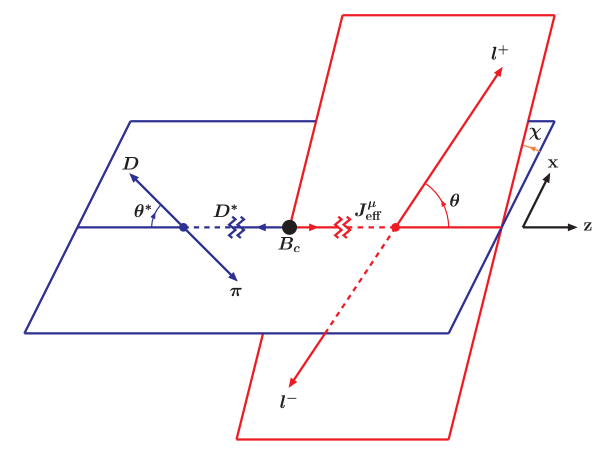
Figure 1: Definition of angles $\theta$, $\theta^{\ast}$ and $\chi$ in the cascade decay $B_{c}\to D^{\ast}(\to D\pi)\bar{l}l$.

Figure 2: Feynman diagram describing the form factors of the decay $B(B_{c})\to K(D,D^{\ast})\bar{l}l$

Let us first consider the polar angle decay distribution differential in the momentum transfer squared $q^{2}$. The polar angle is defined by the angle between ${\bf q}={\bf p}_{1}-{\bf p}_{2}$ and ${\bf k}_{1}$ ($l^{+}l^{-}$ rest frame) as shown in Fig. 2. One has

$$\frac{d^{2}\Gamma}{dq^{2}d\cos\theta} = \frac{|{\bf p_{2}}|\,v}{(2\pi)^{3}\,4\,m_{1}^{3}}\cdot\frac{1}{8}\sum\limits_{\rm pol}|M|^{2}$$ (32)

$$= \frac{G^{2}_{F}}{(2\pi)^{3}}\,(\frac{\alpha|\lambda_{t}|}{2\,\pi})^{2}\frac{|{\bf p_{2}}|\,v}{8m_{1}^{2}}\cdot\frac{1}{2}\biggl{\{}L^{(1)}_{\mu\nu}\cdot(H^{\mu\nu}_{11}+H^{\mu\nu}_{22})$$ (34)

$$- -\frac{1}{2}\,L^{(2)}_{\mu\nu}\cdot(q^{2}\,H^{\mu\nu}_{11}+(q^{2}-4\mu^{2})\,H^{\mu\nu}_{22})+L^{(3)}_{\mu\nu}\cdot(H^{\mu\nu}_{12}+H^{\mu\nu}_{21})\biggr{\}}$$ (36)

where $|{\bf p_{2}}|=\lambda^{1/2}(m_{1}^{2},m_{2}^{2},q^{2})/2m_{1}$ is the momentum of the final meson and $v=\sqrt{1-4\mu^{2}/q^{2}}$ is the lepton velocity both given in the $B(B_{c})$-rest frame. We have introduced lepton and hadron tensors as

$$L^{(1)}_{\mu\nu} = k_{1\mu}k_{2\nu}+k_{2\mu}k_{1\nu}\,,\hskip 28.45274ptL^{(2)}_{\mu\nu}=g_{\mu\nu}\,,\hskip 28.45274ptL^{(3)}_{\mu\nu}=i\varepsilon_{\mu\nu\alpha\beta}k_{1}^{\alpha}k_{2}^{\beta}\,,$$ (37)

$$H_{ij}^{\mu\nu} = T_{i}^{\mu}\,T_{j}^{\dagger\nu}\,.$$ (39)

4 Helicity amplitudes and two-fold distributions

The Lorentz contractions in Eq. (32) can be evaluated in terms of helicity amplitudes as described in Korner:1989qb . First, we define an orthonormal and complete helicity basis $\epsilon^{\mu}(m)$ with the three spin 1 components orthogonal to the momentum transfer $q^{\mu}$, i.e. $\epsilon^{\mu}(m)q_{\mu}=0$ for $m=\pm,0$, and the spin 0 (time)-component $m=t$ with $\epsilon^{\mu}(t)=q^{\mu}/\sqrt{q^{2}}$.

The orthonormality and completeness properties read

$$\epsilon^{\dagger}_{\mu}(m)\epsilon^{\mu}(n)=g_{mn}\,,\hskip 28.45274pt\epsilon_{\mu}(m)\epsilon^{\dagger}_{\nu}(n)g_{mn}=g_{\mu\nu}$$ (40)

with $(m,n=t,\pm,0)$ and $g_{mn}={\rm diag}\,(\,+\,,\,\,-\,,\,\,-\,,\,\,-\,)$. We include the time component polarization vector $\epsilon^{\mu}(t)$ in the set because we want to discuss lepton mass effects in the following.

Using the completeness property we rewrite the contraction of the lepton and hadron tensors in Eq. (32) according to

$$L^{(k)\mu\nu}H_{\mu\nu}^{ij} = L_{\mu^{\prime}\nu^{\prime}}^{(k)}g^{\mu^{\prime}\mu}g^{\nu^{\prime}\nu}H_{\mu\nu}^{ij}=L_{\mu^{\prime}\nu^{\prime}}^{(k)}\epsilon^{\mu^{\prime}}(m)\epsilon^{\dagger\mu}(m^{\prime})g_{mm^{\prime}}\epsilon^{\dagger\nu^{\prime}}(n)\epsilon^{\nu}(n^{\prime})g_{nn^{\prime}}H_{\mu\nu}^{ij}$$ (41)

$$= L^{(k)}(m,n)g_{mm^{\prime}}g_{nn^{\prime}}H^{ij}(m^{\prime},n^{\prime})$$ (43)

where we have introduced the lepton and hadron tensors in the space of the helicity components

$$L^{(k)}(m,n) = \epsilon^{\mu}(m)\epsilon^{\dagger\nu}(n)L^{(k)}_{\mu\nu},\hskip 28.45274ptH^{ij}(m,n)=\epsilon^{\dagger\mu}(m)\epsilon^{\nu}(n)H^{ij}_{\mu\nu}.$$ (44)

The point is that the two tensors can be evaluated in two different Lorentz systems. The lepton tensors $L^{(k)}(m,n)$ will be evaluated in the $\bar{l}l$-CM system whereas the hadron tensors $H^{ij}(m,n)$ will be evaluated in the $B(B_{c})$ rest system.

In the $B(B_{c})$ rest frame one has

$$p^{\mu}_{1} = (\,m_{1}\,,\,\,0,\,\,0,\,\,0\,)\,,$$ (45)

$$p^{\mu}_{2} = (\,E_{2}\,,\,\,0\,,\,\,0\,,\,\,-|{\bf p_{2}}|\,)\,,$$ (46)

$$q^{\mu} = (\,q_{0}\,,\,\,0\,,\,\,0\,,\,\,|{\bf p_{2}}|\,)\,,$$ (47)

where $E_{2}=(m_{1}^{2}+m_{2}^{2}-q^{2})/2m_{1}$ and $q_{0}=(m_{1}^{2}-m_{2}^{2}+q^{2})/2m_{1}$. In the $B(B_{c})$-rest frame the polarization vectors of the effective current read

$$\epsilon^{\mu}(t) = \frac{1}{\sqrt{q^{2}}}(\,q_{0}\,,\,\,0\,,\,\,0\,,\,\,|{\bf p_{2}}|\,)\,,$$ (48)

$$\epsilon^{\mu}(\pm) = \frac{1}{\sqrt{2}}(\,0\,,\,\,\mp 1\,,\,\,-i\,,\,\,0\,)\,,$$ (49)

$$\epsilon^{\mu}(0) = \frac{1}{\sqrt{q^{2}}}(\,|{\bf p_{2}}|\,,\,\,0\,,\,\,0\,,\,\,q_{0}\,)\,.$$ (50)

Using this basis one can express the components of the hadronic tensors through the invariant form factors defined in Eq. (15).

(a) $B(B_{c})\to K(D)$ transition:

$$H^{ij}(m,n)=\left(\epsilon^{\dagger\mu}(m)T^{i}_{\mu}\right)\cdot\left(\epsilon^{\dagger\nu}(n)T^{j}_{\nu}\right)^{\dagger}\equiv H^{i}(m)H^{\dagger j}(n)$$ (51)

The helicity form factors $H^{i}(m)$ are given in terms of the invariant form factors. One has

$$H^{i}(t) = \frac{1}{\sqrt{q^{2}}}(Pq\,{\cal F}^{i}_{+}+q^{2}\,{\cal F}^{i}_{-})\,,$$ (52)

$$H^{i}(\pm) = 0\,,$$ (53)

$$H^{i}(0) = \frac{2\,m_{1}\,|{\bf p_{2}}|}{\sqrt{q^{2}}}\,{\cal F}^{i}_{+}\,.$$ (54)

(b) $B_{c}\to D^{\ast}$ transition:

$$H^{ij}(m,n) = \epsilon^{\dagger\mu}(m)\epsilon^{\nu}(n)H^{ij}_{\mu\nu}=\epsilon^{\dagger\mu}(m)\epsilon^{\nu}(n)T^{i}_{\mu\alpha}\left(-g^{\alpha\beta}+\frac{p_{2}^{\alpha}p_{2}^{\beta}}{m_{2}^{2}}\right)T^{\dagger j}_{\beta\nu}$$ (55)

$$= \epsilon^{\dagger\mu}(m)\epsilon^{\nu}(n)T^{i}_{\mu\alpha}\epsilon_{2}^{\dagger\alpha}(r)\epsilon_{2}^{\beta}(s)\delta_{rs}T^{\dagger j}_{\beta\nu}$$ (56)

$$= \epsilon^{\dagger\mu}(m)\epsilon_{2}^{\dagger\alpha}(r)T^{i}_{\mu\alpha}\cdot\left(\epsilon^{\dagger\nu}(n)\epsilon_{2}^{\dagger\beta}(s)T^{j}_{\nu\beta}\right)^{\dagger}\delta_{rs}=H^{i}(m)H^{\dagger\,j}(n).$$ (57)

From angular momentum conservation one has $r=m$ and $s=n$ for $m,n=\pm,0$ and $r,s=0$ for $m,n=t$. For further evaluation one needs to specify the helicity components $\epsilon_{2}(m)$ $(m=\pm,0)$ of the polarization vector of the $D^{\ast}$. They read

$$\epsilon^{\mu}_{2}(\pm)=\frac{1}{\sqrt{2}}(0\,,\,\,\pm 1\,,\,\,-i\,,\,\,0\,)\,,\hskip 28.45274pt\epsilon^{\mu}_{2}(0)=\frac{1}{m_{2}}(|{\bf p_{2}}|\,,\,\,0\,,\,\,0\,,\,\,-E_{2}\,)\,.$$ (58)

They satisfy the orthonormality and completeness properties:

$$\epsilon_{2}^{\dagger\mu}(r)\epsilon_{2\mu}(s)=-\delta_{rs},\hskip 28.45274pt\epsilon_{2\mu}(r)\epsilon^{\dagger}_{2\nu}(s)\delta_{rs}=-g_{\mu\nu}+\frac{p_{2\mu}p_{2\nu}}{m_{2}^{2}}.$$ (59)

Finally one obtains the non-zero components of the hadron tensors

$$H^{i}(t) = \epsilon^{\dagger\mu}(t)\epsilon_{2}^{\dagger\alpha}(0)T^{i}_{\mu\alpha}\,=\,\frac{1}{m_{1}+m_{2}}\frac{m_{1}\,|{\bf p_{2}}|}{m_{2}\sqrt{q^{2}}}\left(Pq\,(-A^{i}_{0}+A^{i}_{+})+q^{2}A^{i}_{-}\right),$$ (60)

$$H^{i}(\pm) = \epsilon^{\dagger\mu}(\pm)\epsilon_{2}^{\dagger\alpha}(\pm)T^{i}_{\mu\alpha}\,=\,\frac{1}{m_{1}+m_{2}}\left(-Pq\,A^{i}_{0}\pm 2\,m_{1}\,|{\bf p_{2}}|\,V^{i}\right),$$ (61)

$$H^{i}(0) = \epsilon^{\dagger\mu}(0)\epsilon_{2}^{\dagger\alpha}(0)T^{i}_{\mu\alpha}$$ (62)

$$= \frac{1}{m_{1}+m_{2}}\frac{1}{2\,m_{2}\sqrt{q^{2}}}\left(-Pq\,(m_{1}^{2}+m_{2}^{2}-q^{2})\,A^{i}_{0}+4\,m_{1}^{2}\,|{\bf p_{2}}|^{2}\,A^{i}_{+}\right).$$ (63)

The lepton tensors $L^{(k)}(m,n)$ are evaluated in the $\bar{l}l$-CM system ${\bf k}_{1}+{\bf k}_{2}=0$. One has (see Fig. 2)

$$q^{\mu} = (\,\sqrt{q^{2}}\,,\,\,0\,,\,\,0\,,\,\,0\,)\,,$$ (64)

$$k^{\mu}_{1} = (\,E_{1}\,,\,\,|{\bf k_{1}}|\sin\theta\cos\chi\,,\,\,|{\bf k_{1}}|\sin\theta\sin\chi\,,\,\,|{\bf k_{1}}|\cos\theta\,)\,,$$ (65)

$$k^{\mu}_{2} = (\,E_{1}\,,\,\,-|{\bf k_{1}}|\sin\theta\cos\chi\,,\,\,-|{\bf k_{1}}|\sin\theta\sin\chi\,,\,\,-|{\bf k_{1}}|\cos\theta\,)\,,$$ (66)

with $E_{1}=\sqrt{q^{2}}/2$ and $|{\bf k_{1}}|=\sqrt{q^{2}-4\mu^{2}}/2$. The longitudinal and time component polarization vectors in the $\bar{l}l$ rest frame can be read off from Eq. (49) and are given by $\epsilon^{\mu}(0)=(0,0,0,1)$ and $\epsilon(t)=(1,0,0,0)$ whereas the transverse parts remain unchanged from Eq. (49).

The differential $(q^{2},\cos\theta)$ distribution finally reads

$$\frac{d\Gamma(H_{in}\to H_{f}\bar{l}l)}{dq^{2}d(\cos\theta)} = \,\frac{3}{8}\,(1+\cos^{2}\theta)\cdot\frac{1}{2}\left(\frac{d\Gamma_{U}^{11}}{dq^{2}}+\frac{d\Gamma_{U}^{22}}{dq^{2}}\right)$$ (67)

$$+ \frac{3}{4}\,\sin^{2}\theta\cdot\frac{1}{2}\left(\frac{d\Gamma_{L}^{11}}{dq^{2}}+\frac{d\Gamma_{L}^{22}}{dq^{2}}\right)$$ (69)

$$- \,v\cdot\frac{3}{4}\cos\theta\cdot\frac{d\Gamma_{P}^{12}}{dq^{2}}$$ (71)

$$+ \frac{3}{4}\,\sin^{2}\theta\cdot\frac{1}{2}\frac{d\tilde{\Gamma}_{U}^{11}}{dq^{2}}-\frac{3}{8}\,(1+\cos^{2}\theta)\cdot\frac{d\tilde{\Gamma}_{U}^{22}}{dq^{2}}$$ (73)

$$+ \frac{3}{2}\,\cos^{2}\theta\cdot\frac{1}{2}\frac{d\tilde{\Gamma}_{L}^{11}}{dq^{2}}-\frac{3}{4}\,\sin^{2}\theta\cdot\frac{d\tilde{\Gamma}_{L}^{22}}{dq^{2}}+\frac{1}{4}\,\frac{d\tilde{\Gamma}_{S}^{22}}{dq^{2}}\,.$$ (75)

Integrating over $\cos\theta$ one obtains

$$\frac{d\Gamma(H_{in}\to H_{f}\bar{l}l)}{dq^{2}} = \,\frac{1}{2}\left(\frac{d\Gamma_{U}^{11}}{dq^{2}}+\frac{d\Gamma_{U}^{22}}{dq^{2}}+\frac{d\Gamma_{L}^{11}}{dq^{2}}+\frac{d\Gamma_{L}^{22}}{dq^{2}}\right)$$ (76)

$$+ \frac{1}{2}\frac{d\tilde{\Gamma}_{U}^{11}}{dq^{2}}-\frac{d\tilde{\Gamma}_{U}^{22}}{dq^{2}}+\frac{1}{2}\frac{d\tilde{\Gamma}_{L}^{11}}{dq^{2}}-\frac{d\tilde{\Gamma}_{L}^{22}}{dq^{2}}+\frac{1}{2}\,\frac{d\tilde{\Gamma}_{S}^{22}}{dq^{2}}\,,$$ (78)

where the partial helicity rates $d\Gamma_{X}^{ij}/dq^{2}$ and $d\tilde{\Gamma}_{X}^{ij}/dq^{2}$ ($X=U,L,P,S;\,i,j=1,2$) are defined as

$$\frac{d\Gamma_{X}^{ij}}{dq^{2}}=\frac{G^{2}_{F}}{(2\pi)^{3}}\left(\frac{\alpha|\lambda_{t}|}{2\pi}\right)^{2}\frac{|{\bf p_{2}}|\,q^{2}\,v}{12\,m_{1}^{2}}\,H_{X}^{ij}\,,\hskip 28.45274pt\frac{d\tilde{\Gamma}_{X}^{ij}}{dq^{2}}=\frac{2\,\mu^{2}}{q^{2}}\,\frac{d\Gamma_{X}^{ij}}{dq^{2}}\,.$$ (79)

The relevant bilinear combinations of the helicity amplitudes are defined in Table 2.

Table 2: Bilinear combinations of the helicity amplitudes that enter in the four-fold decay distribution Eq. (79).

Definition	Property	Title
$H_{U}^{ij}={\rm Re}\left(H_{+}^{i}H_{+}^{\dagger\,j}\right)+{\rm Re}\left(H_{-}^{i}H_{-}^{\dagger\,j}\right)$	$H_{U}^{ij}=H_{U}^{ji}$	Unpolarized-transverse
$H_{IU}^{ij}={\rm Im}\left(H_{+}^{i}H_{+}^{\dagger\,j}\right)+{\rm Im}\left(H_{-}^{i}H_{-}^{\dagger\,j}\right)$	$H_{IU}^{ij}=-H_{IU}^{ji}$
$H_{P}^{ij}={\rm Re}\left(H_{+}^{i}H_{+}^{\dagger\,j}\right)-{\rm Re}\left(H_{-}^{i}H_{-}^{\dagger\,j}\right)$	$H_{P}^{ij}=H_{P}^{ji}$	Parity-odd
$H_{IP}^{ij}={\rm Im}\left(H_{+}^{i}H_{+}^{\dagger\,j}\right)-{\rm Im}\left(H_{-}^{i}H_{-}^{\dagger\,j}\right)$	$H_{IP}^{ij}=-H_{IP}^{ji}$
$H_{T}^{ij}={\rm Re}\left(H_{+}^{i}H_{-}^{\dagger\,j}\right)$		Transverse-interference
$H_{IT}^{ij}={\rm Im}\left(H_{+}^{i}H_{-}^{\dagger\,j}\right)$
$H_{L}^{ij}={\rm Re}\left(H_{0}^{i}H_{0}^{\dagger\,j}\right)$	$H_{L}^{ij}=H_{L}^{ji}$	Longitudinal
$H_{IL}^{ij}={\rm Im}\left(H_{0}^{i}H_{0}^{\dagger\,j}\right)$	$H_{IL}^{ij}=-H_{IL}^{ji}$
$H_{S}^{ij}=3\,{\rm Re}\left(H_{t}^{i}H_{t}^{\dagger\,j}\right)$	$H_{S}^{ij}=H_{S}^{ji}$	Scalar
$H_{IS}^{ij}=3\,{\rm Im}\left(H_{t}^{i}H_{t}^{\dagger\,j}\right)$	$H_{IS}^{ij}=-H_{IS}^{ji}$
$H_{SL}^{ij}={\rm Re}\left(H_{t}^{i}H_{0}^{\dagger\,j}\right)$		Scalar-Longitudinal-
		interference
$H_{ISL}^{ij}={\rm Im}\left(H_{t}^{i}H_{0}^{\dagger\,j}\right)$
$H_{I}^{ij}=\frac{1}{2}\,\left[{\rm Re}\left(H_{+}^{i}H_{0}^{\dagger\,j}\right)+{\rm Re}\left(H_{-}^{i}H_{0}^{\dagger\,j}\right)\right]$		transverse-longitudinal-
		Interference
$H_{II}^{ij}=\frac{1}{2}\,\left[{\rm Im}\left(H_{+}^{i}H_{0}^{\dagger\,j}\right)+{\rm Im}\left(H_{-}^{i}H_{0}^{\dagger\,j}\right)\right]$
$H_{A}^{ij}=\frac{1}{2}\,\left[{\rm Re}\left(H_{+}^{i}H_{0}^{\dagger\,j}\right)-{\rm Re}\left(H_{-}^{i}H_{0}^{\dagger\,j}\right)\right]$		parity-Asymmetric
$H_{IA}^{ij}=\frac{1}{2}\,\left[{\rm Im}\left(H_{+}^{i}H_{0}^{\dagger\,j}\right)-{\rm Im}\left(H_{-}^{i}H_{0}^{\dagger\,j}\right)\right]$
$H_{ST}^{ij}=\frac{1}{2}\,\left[{\rm Re}\left(H_{+}^{i}H_{t}^{\dagger\,j}\right)+{\rm Re}\left(H_{-}^{i}H_{t}^{\dagger\,j}\right)\right]$		Scalar-Transverse-
		interference
$H_{IST}^{ij}=\frac{1}{2}\,\left[{\rm Im}\left(H_{+}^{i}H_{t}^{\dagger\,j}\right)+{\rm Im}\left(H_{-}^{i}H_{t}^{\dagger\,j}\right)\right]$
$H_{SA}^{ij}=\frac{1}{2}\,\left[{\rm Re}\left(H_{+}^{i}H_{t}^{\dagger\,j}\right)-{\rm Re}\left(H_{-}^{i}H_{t}^{\dagger\,j}\right)\right]$		Scalar-Asymmetric-
		interference
$H_{ISA}^{ij}=\frac{1}{2}\,\left[{\rm Im}\left(H_{+}^{i}H_{t}^{\dagger\,j}\right)-{\rm Im}\left(H_{-}^{i}H_{t}^{\dagger\,j}\right)\right]$

5 The four-fold angle distribution in the cascade decay
$B_{c}\to D^{\ast}(\to D\pi)\bar{l}l$.

The lepton-hadron correlation function $L_{\mu\nu}H^{\mu\nu}$ reveals even more structure when one uses the cascade decay $B_{c}\to D^{\ast}(\to D\pi)\bar{l}l$ to analyze the polarization of the $D^{\ast}$. The hadron tensor now reads

$$H^{ij}_{\mu\nu}=T^{i}_{\mu\alpha}(T^{j}_{\nu\beta})^{\dagger}\frac{3}{2\,|{\bf p_{3}}|}{\rm Br}(K^{\ast}\to K\pi)p_{3\alpha^{\prime}}p_{3\beta^{\prime}}S^{\alpha\alpha^{\prime}}(p_{2})S^{\beta\beta^{\prime}}(p_{2})$$ (80)

where $S^{\alpha\alpha^{\prime}}(p_{2})=-g^{\alpha\alpha^{\prime}}+p_{2}^{\alpha}p_{2}^{\alpha^{\prime}}/m_{2}^{2}$ is the standard spin 1 tensor, $p_{2}=p_{3}+p_{4}$, $p_{3}^{2}=m_{D}^{2}$, $p_{4}^{2}=m_{\pi}^{2}$, and $p_{3}$ and $p_{4}$ are the momenta of the $D$ and the $\pi$, respectively. The relative configuration of the ($D,\pi$)- and ($\bar{l}l$)-planes is shown in Fig. 2.

In the rest frame of the $D^{\ast}$ one has

$$p^{\mu}_{2} = (m_{D^{\ast}},\vec{0}),$$ (81)

$$p^{\mu}_{3} = (\,E_{D}\,,\,\,|{\bf p_{3}}|\,\sin\theta^{\ast}\,,\,\,0\,,\,\,-|{\bf p_{3}}|\,\cos\theta^{\ast}\,)\,,$$ (82)

$$p^{\mu}_{4} = (\,E_{\pi}\,,\,\,-|{\bf p_{3}}|\,\sin\theta^{\ast}\,,\,\,0\,,\,\,|{\bf p_{3}}|\,\cos\theta^{\ast}\,)\,,$$ (83)

$$|{\bf p_{3}}| = \lambda^{1/2}(m_{D^{\ast}}^{2},m_{D}^{2},m_{\pi}^{2})/(2\,m_{D^{\ast}})\,.$$ (84)

Without loss of generality we set the azimuthal angle $\chi^{\ast}$ of the $(D,\pi)$-plane to zero. According to Eq. (58) the rest frame polarization vectors of the $D^{\ast}$ are given by

$$\epsilon^{\mu}_{2}(\pm)=\frac{1}{\sqrt{2}}(\,0\,,\,\,\pm\,,\,\,-i\,,\,\,0\,)\,,\hskip 28.45274pt\epsilon^{\mu}_{2}(0)=(\,0\,,\,\,0\,,\,\,0\,,\,\,-1)\,.$$ (85)

The spin 1 tensor $S^{\alpha\alpha^{\prime}}(p_{2})$ is then written as

$$S^{\alpha\alpha^{\prime}}(p_{2})=-g^{\alpha\alpha^{\prime}}+\frac{p_{2}^{\alpha}p_{2}^{\alpha^{\prime}}}{m_{2}^{2}}=\sum\limits_{m=\pm,0}\epsilon_{2}^{\alpha}(m)\epsilon_{2}^{\dagger\alpha^{\prime}}(m)$$ (86)

Following basically the same trick as in Eq. (43) the contraction of the lepton and hadron tensors may be written through helicity components as

$$L^{(k)\mu\nu}H^{ij}_{\mu\nu} = \epsilon^{\mu^{\prime}}(m)\epsilon^{\dagger\nu^{\prime}}(n)L^{k}_{\mu^{\prime}\nu^{\prime}}g_{mn^{\prime}}g_{nn^{\prime}}\epsilon^{\dagger\mu}(m^{\prime})\epsilon^{\nu}(n^{\prime})H^{ij}_{\mu\nu}$$ (87)

$$= L^{k}(m,n)g_{mm^{\prime}}g_{nn^{\prime}}\left(\epsilon^{\dagger\mu}(m^{\prime})\epsilon_{2}^{\dagger\alpha}(r)T^{i}_{\mu\alpha}\right)\left(\epsilon^{\dagger\nu}(n^{\prime})\epsilon_{2}^{\dagger\alpha}(s)T^{j}_{\nu\beta}\right)^{\dagger}$$ (88)

$$\times p_{3}\epsilon_{2}(r)\cdot p_{3}\epsilon_{2}^{\dagger}(s)\frac{3\,{\rm Br}(D^{\ast}\to D\pi)}{2\,|{\bf p_{3}}|}$$ (89)

$$= \frac{3\,{\rm Br}(D^{\ast}\to D\pi)}{2\,|{\bf p_{3}}|}\,\biggl{(}L^{k}(t,t)|H^{ij}(t)|^{2}\cdot(p_{3}\epsilon_{2}^{\dagger}(0))^{2}$$ (90)

$$+ \sum\limits_{m,n=\pm,0}L^{k}(m,n)H^{i}(m)H^{\dagger j}(n)\cdot p_{3}\epsilon_{2}(m)\cdot p_{3}\epsilon_{2}^{\dagger}(n)$$ (91)

$$- \sum\limits_{n=\pm,0}L^{k}(t,n)H^{i}(t)H^{\dagger j}(n)\cdot p_{3}\epsilon_{2}(0)\cdot p_{3}\epsilon_{2}^{\dagger}(n)$$ (92)

$$- \sum\limits_{m=\pm,0}L^{k}(m,t)H^{i}(m)H^{\dagger j}(t)\cdot p_{3}\epsilon_{2}(m)\cdot p_{3}\epsilon_{2}^{\dagger}(0)\biggr{)}$$ (93)

Using these results one obtains the full four-fold angular decay distribution

$$\frac{d\Gamma(B_{c}\to D^{\ast}(\to D\pi)\bar{l}l)}{dq^{2}\,d\cos\theta\,d(\chi/2\pi)\,d\cos\theta^{\ast}}={\rm Br}(D^{\ast}\to D\pi)$$ (94)

(95)

$$\times\left\{\frac{3}{8}\,(1+\cos^{2}\theta)\cdot\frac{3}{4}\,\sin^{2}\theta^{\ast}\cdot\frac{1}{2}\left(\frac{d\Gamma_{U}^{11}}{dq^{2}}+\frac{d\Gamma_{U}^{22}}{dq^{2}}\right)\right.$$ (96)

$$+\frac{3}{4}\,\sin^{2}\theta\cdot\,\frac{3}{2}\,\cos^{2}\theta^{\ast}\cdot\frac{1}{2}\left(\frac{d\Gamma_{L}^{11}}{dq^{2}}+\frac{d\Gamma_{L}^{22}}{dq^{2}}\right)$$ (97)

$$-\frac{3}{4}\,\sin^{2}\theta\cdot\cos 2\chi\cdot\frac{3}{4}\,\sin^{2}\theta^{\ast}\cdot\frac{1}{2}\left(\frac{d\Gamma_{T}^{11}}{dq^{2}}+\frac{d\Gamma_{T}^{22}}{dq^{2}}\right)$$ (98)

$$+\frac{9}{16}\,\sin 2\theta\cdot\cos\chi\cdot\sin 2\theta^{\ast}\cdot\frac{1}{2}\left(\frac{d\Gamma_{I}^{11}}{dq^{2}}+\frac{d\Gamma_{I}^{22}}{dq^{2}}\right)$$ (99)

$$+v\,\left[-\frac{3}{4}\,\cos\theta\cdot\,\frac{3}{4}\,\sin^{2}\theta^{\ast}\cdot\frac{d\Gamma_{P}^{12}}{dq^{2}}\right.$$ (100)

$$-\frac{9}{8}\,\sin\theta\cdot\cos\chi\cdot\sin 2\theta^{\ast}\cdot\frac{1}{2}\left(\frac{d\Gamma_{A}^{12}}{dq^{2}}+\frac{d\Gamma_{A}^{21}}{dq^{2}}\right)$$ (101)

$$\left.+\frac{9}{16}\,\sin\theta\cdot\sin\chi\cdot\sin 2\theta^{\ast}\cdot\left(\frac{d\Gamma_{II}^{12}}{dq^{2}}+\frac{d\Gamma_{II}^{21}}{dq^{2}}\right)\right]$$ (102)

$$-\frac{9}{32}\,\sin 2\theta\cdot\sin\chi\cdot\sin 2\theta^{\ast}\cdot\left(\frac{d\Gamma_{IA}^{11}}{dq^{2}}+\frac{d\Gamma_{IA}^{22}}{dq^{2}}\right)$$ (103)

$$+\frac{9}{32}\,\sin^{2}\theta\cdot\sin 2\chi\cdot\sin^{2}\theta^{\ast}\cdot\left(\frac{d\Gamma_{IT}^{11}}{dq^{2}}+\frac{d\Gamma_{IT}^{22}}{dq^{2}}\right)$$ (104)

$$+\frac{3}{4}\,\sin^{2}\theta\cdot\frac{3}{4}\,\sin^{2}\theta^{\ast}\cdot\frac{1}{2}\cdot\frac{d\tilde{\Gamma}_{U}^{11}}{dq^{2}}-\frac{3}{8}\,(1+\cos^{2}\theta)\cdot\frac{3}{4}\,\sin^{2}\theta^{\ast}\cdot\frac{d\tilde{\Gamma}_{U}^{22}}{dq^{2}}$$ (105)

$$+\frac{3}{2}\,\cos^{2}\theta\cdot\frac{3}{2}\,\cos^{2}\theta^{\ast}\cdot\frac{1}{2}\cdot\frac{d\tilde{\Gamma}_{L}^{11}}{dq^{2}}-\frac{3}{4}\,\sin^{2}\theta\cdot\frac{3}{2}\,\cos^{2}\theta^{\ast}\cdot\frac{d\tilde{\Gamma}_{L}^{22}}{dq^{2}}$$ (106)

$$+\frac{3}{4}\,\sin^{2}\theta\cdot\cos 2\chi\cdot\frac{3}{4}\,\sin^{2}\theta^{\ast}\cdot\left(\frac{d\tilde{\Gamma}_{T}^{11}}{dq^{2}}+\frac{d\tilde{\Gamma}_{T}^{22}}{dq^{2}}\right)$$ (107)

$$-\frac{9}{8}\,\sin 2\theta\cdot\cos\chi\cdot\sin 2\theta^{\ast}\cdot\frac{1}{2}\left(\frac{d\tilde{\Gamma}_{I}^{11}}{dq^{2}}+\frac{d\tilde{\Gamma}_{I}^{22}}{dq^{2}}\right)+\frac{3}{2}\,\cos^{2}\theta^{\ast}\cdot\frac{1}{4}\frac{d\tilde{\Gamma}_{S}^{22}}{dq^{2}}$$ (108)

$$+\frac{9}{16}\,\sin 2\theta\cdot\sin\chi\cdot\sin 2\theta^{\ast}\cdot\left(\frac{d\Gamma_{IA}^{11}}{dq^{2}}+\frac{d\Gamma_{IA}^{22}}{dq^{2}}\right)$$ (109)

$$\left.-\frac{9}{16}\,\sin^{2}\theta\cdot\sin 2\chi\cdot\sin^{2}\theta^{\ast}\cdot\left(\frac{d\Gamma_{IT}^{11}}{dq^{2}}+\frac{d\Gamma_{IT}^{22}}{dq^{2}}\right)\right\}$$ (110)

Integrating Eq. (94) over $\cos\theta^{\ast}$ and $\chi$ one recovers the two-fold ($q^{2},\cos\theta$) distribution of Eq. (67). Note that a similar four-fold distribution has also been obtained in Refs.(Kruger:1999xa ,Kim:2000dq ,Ali:2002qc , Chen:2002 ,Melikhov:1998cd ) using, however, the zero lepton mass approximation. If there are sufficient data one can attempt to fit them to the full four-fold decay distribution and thereby extract the values of the coefficient functions $d\Gamma_{X}/dq^{2}$ and, in the case $l=\tau$ the coefficient functions $d\tilde{\Gamma}_{X}/dq^{2}$. Instead of considering the full four-fold decay distribution one can analyze single angle distributions by integrating out two of the remaining angles as done in Ref. Faessler:2002ut .

6 Model form factors

We will employ the relativistic constituent quark model Ivanov:1996pz ; Ivanov:1999ic to calculate the form factors relevant to the decays $B\to K\bar{l}l$ and $B_{c}\to D(D^{\ast})\bar{l}l$. This model is based on an effective interaction Lagrangian which describes the coupling between hadrons and their constituent quarks.

For example, the coupling of the meson $H$ to its constituent quarks $q_{1}$ and $\bar{q}_{2}$ is given by the Lagrangian

$${\cal L}_{{\rm int}}(x)=g_{H}H(x)\int\!\!dx_{1}\!\!\int\!\!dx_{2}F_{H}(x,x_{1},x_{2})\bar{q}(x_{1})\Gamma_{H}\lambda_{H}q(x_{2})\,.$$ (111)

Here, $\lambda_{H}$ and $\Gamma_{H}$ are Gell-Mann and Dirac matrices which entail the flavor and spin quantum numbers of the meson field $H(x)$. The function $F_{H}$ is related to the scalar part of the Bethe-Salpeter amplitude and characterizes the finite size of the meson. The function $F_{H}$ must be invariant under the translation $F_{H}(x+a,x_{1}+a,x_{2}+a)=F_{H}(x,x_{1},x_{2})$.

In our previous papers we have used the so-called impulse approximation for the evaluation of the Feynman diagrams. In the impulse approximation one omits a possible dependence of the vertex functions on external momenta. The impulse approximation therefore entails a certain dependence on how loop momenta are routed through the diagram at hand. This problem no longer exists in the present full treatment where the impulse approximation is no longer used. In the present calculation we will use a particular form of the vertex function given by

$$F_{H}(x,x_{1},x_{2})=\delta\biggl{(}x-\frac{m_{1}x_{1}+m_{2}x_{2}}{m_{1}+m_{2}}\biggr{)}\Phi_{H}((x_{1}-x_{2})^{2}).$$ (112)

where $m_{1}$ and $m_{2}$ are the constituent quark masses. The vertex function $F_{H}$ evidently satisfies the above translational invariance condition. As mentioned before we no longer use the impulse approximation in the present calculation.

The coupling constants $g_{H}$ in Eq. (111) are determined by the so called compositeness condition proposed in SWH and extensively used in Efimov:zg . The compositeness condition means that the renormalization constant of the meson field is set equal to zero

$$Z_{H}=1-\frac{3g^{2}_{H}}{4\pi^{2}}\tilde{\Pi}^{\prime}_{H}(m^{2}_{H})=0$$ (113)

where $\tilde{\Pi}^{\prime}_{H}$ is the derivative of the meson mass operator. For the pseudoscalar and vector mesons treated in this paper one has

$$\tilde{\Pi}^{\prime}_{P}(p^{2}) = \frac{1}{2p^{2}}\,p^{\alpha}\frac{d}{dp^{\alpha}}\,\int\!\!\frac{d^{4}k}{4\pi^{2}i}\tilde{\Phi}^{2}_{P}(-k^{2})$$

$$\times {\rm tr}\biggl{[}\gamma^{5}S_{1}(\not\!k+w_{21}\not\!p)\gamma^{5}S_{2}(\not\!k-w_{12}\not\!p)\biggr{]}$$

$$\tilde{\Pi}^{\prime}_{V}(p^{2}) = \frac{1}{3}\biggl{[}g^{\mu\nu}-\frac{p^{\mu}p^{\nu}}{p^{2}}\biggr{]}\frac{1}{2p^{2}}\,p^{\alpha}\frac{d}{dp^{\alpha}}\,\int\!\!\frac{d^{4}k}{4\pi^{2}i}\tilde{\Phi}^{2}_{V}(-k^{2})$$

$$\times {\rm tr}\biggl{[}\gamma^{\nu}S_{1}(\not\!k+w_{21}\not\!p)\gamma^{\mu}S_{2}(\not\!k-w_{12}\not\!p)\biggr{]}$$

where $w_{ij}=m_{j}/(m_{i}+m_{j})$.

The leptonic decay constant $f_{P}$ is calculated from

$$\frac{3g_{P}}{4\pi^{2}}\,\int\!\!\frac{d^{4}k}{4\pi^{2}i}\tilde{\Phi}_{P}(-k^{2}){\rm tr}\biggl{[}O^{\mu}S_{1}(\not\!k+w_{21}\not\!p)\gamma^{5}S_{2}(\not\!k-w_{12}\not\!p)\biggr{]}=f_{P}\,p^{\mu}.$$ (114)

The transition form factors $P(p_{1})\to P(p_{2}),V(p_{2})$ can be calculated from the Feynman integral corresponding to the diagram of Fig. 2:

$$\Lambda^{\Gamma^{\mu}}(p_{1},p_{2}) = \frac{3g_{P}g_{P^{\prime}(V)}}{4\pi^{2}}\,\int\!\!\frac{d^{4}k}{4\pi^{2}i}\tilde{\Phi}_{P}(-(k+w_{13}\,p_{1})^{2})\,\tilde{\Phi}_{P^{\prime}(V)}(-(k+w_{23}\,p_{2})^{2})$$ (115)

$$\times {\rm tr}\biggl{[}S_{2}(\not\!k+\not\!p_{2})\Gamma^{\mu}S_{1}(\not\!k+\not\!p_{1})\gamma^{5}S_{3}(\not\!k)\Gamma_{\rm out}\biggr{]}$$ (116)

where $\Gamma^{\mu}=\gamma^{\mu},\,\gamma^{\mu}\gamma^{5},\,$ $i\sigma^{\mu\nu}q_{\nu},\,$ or $i\sigma^{\mu\nu}q_{\nu}\gamma^{5}$ and $\Gamma_{\,P^{\prime},V}=\gamma^{5},\,\gamma_{\nu}\epsilon_{2}^{\nu}.$

We use the local quark propagators

$$S_{i}(\not\!k)=\frac{1}{m_{i}-\not\!k}\,,$$ (117)

where $m_{i}$ is the constituent quark mass. We do not introduce a new notation for constituent quark masses in order to distinguish them from the current quark masses used in the effective Hamiltonian and Wilson coefficients as described in Sec. II because it should always be clear from the context which set of masses is being referred to. As discussed in Ivanov:1996pz ; Ivanov:1999ic , we assume that

$$m_{H}<m_{1}+m_{2}$$ (118)

in order to avoid the appearance of imaginary parts in the physical amplitudes.

The fit values for the constituent quark masses are taken from our papers Ivanov:1996pz ; Ivanov:1999ic and are given in Eq. (119).

$$\begin{array}[]{ccccc}m_{u}&m_{s}&m_{c}&m_{b}&\\ \hline\cr$\ \ 0.235\ \ $&$\ \ 0.333\ \ $&$\ \ 1.67\ \ $&$\ \ 5.06\ \ $&$\ \ {\rm GeV} $\\ \end{array}$$ (119)

It is readily seen that the constraint Eq. (118) holds true for the low-lying flavored pseudoscalar mesons but is no longer true for the vector mesons. In the case of the heavy mesons $D^{\ast}$ and $B^{\ast}$ we will employ identical masses for the vector mesons and the pseudoscalar mesons for the calculation of matrix elements in Eqs. (113),(114) and (116). It is a quite reliable approximation because of $(m_{D^{\ast}}-m_{D})/m_{D}\sim 7\%$ and $(m_{B^{\ast}}-m_{B})/m_{B}\sim 1\%$. In this vein, our model was successfully developed for the study of light hadrons (e.g., pion, kaon, baryon octet, $\Delta$-resonance), heavy-light hadrons (e.g., $D$, $D_{s}$, $B$ and $B_{s}$-mesons, $\Lambda_{Q}$, $\Sigma_{Q}$, $\Xi_{Q}$ and $\Omega_{Q}$-baryons) and double heavy hadrons (e.g, $J/\Psi$, $\Upsilon$ and $B_{c}$-mesons, $\Xi_{QQ}$ and $\Omega_{QQ}$ baryons) Ivanov:1996pz ; Ivanov:1999ic . To extend our approach to other hadrons we had to introduce extra model parameters or do some approximations, like, e.g., to introduce the cutoff parameter for external hadron momenta to guarantee the fulfillment of the mentioned above ”threshold inequality”. Therefore, at the present stage we can not apply our approach for the study of rare decays involving $K^{\ast}$ mesons. Probably, it will be a subject of our future investigations.

We employ a Gaussian for the vertex function $\tilde{\Phi}_{H}(k^{2}_{E}/\Lambda^{2}_{H})=\exp(-k^{2}_{E}/\Lambda^{2}_{H})$ where $k_{E}$ is the Euclidean momentum and determine the size parameters $\Lambda^{2}_{H}$ by a fit to the experimental data, when available, or to lattice simulations for the leptonic decay constants. The quality of the fit can be seen from Table 3. The branching ratios of the semileptonic decays are shown in Table 4. The numerical values for $\Lambda_{H}$ are $\Lambda_{\pi}=1$ GeV, $\Lambda_{K}=1.6$ GeV, $\Lambda_{D}=2$ GeV and $\Lambda_{B}=2.25$ GeV for all $K$, $D$ and $B$ partners, respectively.

Table 3: Leptonic decay constants $f_{H}$ (MeV) used in the least-square fit. The values are taken either from PDG Hagiwara:in or from the Lattice Ryan : quenched (upper line)
and unquenched (lower line).

Meson	This model	Expt/Lattice
$\pi^{+}$	131	$130.7\pm 0.1\pm 0.36$
$K^{+}$	161	$159.8\pm 1.4\pm 0.44$
$D^{+}$	211	203$\pm$ 14
		226$\pm$ 15
$D^{+}_{s}$	222	230$\pm$ 14
		250$\pm$ 30
$B^{+}$	180	173$\pm$ 23
		198$\pm$ 30
$B^{0}_{s}$	196	200$\pm$ 20
		230$\pm$ 30
$B^{+}_{c}$	398

Table 4: Semileptonic decay branching ratios.

Meson	This model	Expt.
$\pi^{+}\to\pi^{0}l^{+}\nu$	$1.03\cdot 10^{-8}$	$(1.025\pm 0.034)\cdot 10^{-8}$
$K^{+}\to\pi^{0}l^{+}\nu$	$4.62\cdot 10^{-2}$	$(4.82\pm 0.06)\cdot 10^{-2}$
$B^{+}\to\bar{D}^{0}l^{+}\nu$	$2.40\cdot 10^{-2}$	$(2.15\pm 0.22)\cdot 10^{-2}$
$B^{+}\to\bar{D}^{\ast\,0}l^{+}\nu$	$5.60\cdot 10^{-2}$	$(5.3\pm 0.8)\cdot 10^{-2}$
$B_{c}^{+}\to D^{0}l^{+}\nu$	$2.05\cdot 10^{-5}$
$B_{c}^{+}\to D^{\ast\,0}l^{+}\nu$	$3.60\cdot 10^{-5}$

We are now in a position to present our results for the $B(B_{c})\to K(D,D^{\ast})$ form factors. We have used the technique outlined in our previous papers Ivanov:1996pz ; Ivanov:1999ic for the numerical evaluation of the Feynman integrals in Eq. (116). The results of our numerical calculations are well represented by the parametrization

$$F(s)=\frac{F(0)}{1-as+bs^{2}}\,.$$ (120)

Using such a parametrization facilitates further integrations. The values of $F(0)$, $a$ and $b$ are listed in Tables 5.

Table 5: Parameter values for the approximated form factors
$F(s)=F(0)/(1-as+bs^{2})$  $(s=q^{2}/m_{B}^{2})$.

$B\to K\bar{l}l$	$F_{+}$	$F_{-}$	$F_{T}$
$F(0)$	0.357	-0.275	0.337
$a$	1.011	1.050	1.031
$b$	0.042	0.067	0.051

$B_{c}\to D(D^{\ast})\bar{l}l$	$F_{+}$	$F_{-}$	$F_{T}$	$A_{0}$	$A_{+}$	$A_{-}$	$V$	$a_{0}$	$a_{+}$	$g$
$F(0)$	0.186	-0.190	0.275	0.279	0.156	-0.321	0.290	0.178	0.178	0.179
$a$	2.48	2.44	2.40	1.30	2.16	2.41	2.40	1.21	2.14	2.51
$b$	1.62	1.54	1.49	0.149	1.15	1.51	1.49	0.125	1.14	1.67

At the end of this section we would like to discuss the impulse approximation used in our previous papers Ivanov:1996pz ; Ivanov:1999ic . It was simply assumed that the vertex functions depend only on the loop momentum flowing through the vertex. The explicit translational invariant vertex function in Eq. (112) allows one to check the reliability of this approximation. We found that the results obtained with and without the impulse approximation are rather close to each other except for the heavy-to-light form factors. We consider the $B\to\pi$-transition as an example to illustrate this point. The calculated values of the $F_{+}^{B\pi}(q^{2})$ form factor at $q^{2}=0$ are

$$F_{+}^{B\pi}(0)=\left\{\begin{array}[]{ll}0.27&\mbox{exact}\\ &\\ 0.48&\mbox{impulse approximation}\end{array}\right.$$

One can see that the value of the form factor at $q^{2}=0$ calculated without the impulse approximation is considerably smaller than when calculated with the impulse approximation. Its value is close to the value of QCD SR estimates, see, for example, Bagan:1997bp : $F_{+}^{B\pi}(0)=0.30$.

7 Numerical results

We list our numerical results for the branching ratios in Table 6. When comparing the values of the branching ratios with those obtained in Ali:1999mm and Geng:2001vy one finds that they almost agree with each other.

Table 6: Decay branching ratios without(with) long distance contributions.

Ref.	${\rm Br}(B\to K\,\mu^{+}\mu^{-})$	${\rm Br}(B\to K\,\tau^{+}\tau^{-})$	${\rm Br}(B\to K\,\bar{\nu}\nu)$
Ali:1999mm	$0.57\cdot 10^{-6}$	$1.3\cdot 10^{-7}$
Ali:2001jg	$(0.35\pm 0.12)\cdot 10^{-6}$
Melikhov:1997wp	$0.44\cdot 10^{-6}$	$1.0\cdot 10^{-7}$	$5.6\cdot 10^{-6}$
Geng:1996	$0.5\cdot 10^{-6}$	$1.3\cdot 10^{-7}$
our	$0.55\,(0.51)\cdot 10^{-6}$	$1.01\,(0.87)\cdot 10^{-7}$	$4.19\cdot 10^{-6}$

	our	Geng:2001vy
${\rm Br}(B_{c}\to D_{d}\,\mu^{+}\mu^{-})$	$0.44\,(0.38)\cdot 10^{-8}$	$0.41\,(0.33)\cdot 10^{-8}$
${\rm Br}(B_{c}\to D_{d}^{\ast}\,\mu^{+}\mu^{-})$	$0.71\,(0.58)\cdot 10^{-8}$	$1.01\,(0.78)\cdot 10^{-8}$
${\rm Br}(B_{c}\to D_{s}\,\mu^{+}\mu^{-})$	$0.97\,(0.86)\cdot 10^{-7}$	$1.36\,(1.12)\cdot 10^{-7}$
${\rm Br}(B_{c}\to D_{s}^{\ast}\,\mu^{+}\mu^{-})$	$1.76\,(1.41)\cdot 10^{-7}$	$4.09\,(3.14)\cdot 10^{-7}$
${\rm Br}(B_{c}\to D_{d}\,\tau^{+}\tau^{-})$	$0.11\,(0.09)\cdot 10^{-8}$	$0.13\,(0.11)\cdot 10^{-8}$
${\rm Br}(B_{c}\to D_{d}^{\ast}\,\tau^{+}\tau^{-})$	$0.11\,(0.08)\cdot 10^{-8}$	$0.18\,(0.13)\cdot 10^{-8}$
${\rm Br}(B_{c}\to D_{s}\,\tau^{+}\tau^{-})$	$0.22\,(0.18)\cdot 10^{-7}$	$0.34\,(0.27)\cdot 10^{-7}$
${\rm Br}(B_{c}\to D_{s}^{\ast}\,\tau^{+}\tau^{-})$	$0.22\,(0.15)\cdot 10^{-7}$	$0.51\,(0.34)\cdot 10^{-7}$
${\rm Br}(B_{c}\to D_{d}\,\bar{\nu}\nu)$	$3.28\cdot 10^{-8}$
${\rm Br}(B_{c}\to D_{d}^{\ast}\,\bar{\nu}\nu)$	$5.78\cdot 10^{-8}$
${\rm Br}(B_{c}\to D_{s}\,\bar{\nu}\nu)$	$0.73\cdot 10^{-6}$
${\rm Br}(B_{c}\to D_{s}^{\ast}\,\bar{\nu}\nu)$	$1.42\cdot 10^{-6}$

References

- (1) R. Barate et al. [ALEPH Collaboration], Phys. Lett. B 429, 169 (1998).
- (2) K. Abe et al. [Belle Collaboration], Phys. Lett. B 511, 151 (2001).
- (3) S. Chen et al. [CLEO Collaboration], Phys. Rev. Lett. 87, 251807 (2001).
- (4) A. Ali, E. Lunghi, C. Greub and G. Hiller, Phys. Rev. D 66, 034002 (2002).
- (5) K. Abe et al. [BELLE Collaboration], Phys. Rev. Lett. 88, 021801 (2002).
- (6) F. Abe et al. [CDF Collaboration], Phys. Rev. Lett. 81, 2432 (1998); Phys. Rev. D 58, 112004 (1998).
- (7) G. Buchalla, A. J. Buras and M. E. Lautenbacher, Rev. Mod. Phys. 68, 1125 (1996). A. J. Buras and M. Munz, Phys. Rev. D 52, 186 (1995).
- (8) A. Ali, P. Ball, L. T. Handoko and G. Hiller, Phys. Rev. D 61, 074024 (2000).
- (9) C. Greub, A. Ioannisian and D. Wyler, Phys. Lett. B 346, 149 (1995).
- (10) P. Colangelo, F. De Fazio, P. Santorelli and E. Scrimieri, Phys. Rev. D 53, 3672 (1996) [Erratum-ibid. D 57, 3186 (1998)].
- (11) D. Melikhov, N. Nikitin and S. Simula, Phys. Rev. D 57, 6814 (1998).
- (12) T. M. Aliev, M. K. Cakmak, A. Ozpineci and M. Savci, Phys. Rev. D 64, 055007 (2001); T. M. Aliev, M. Savci, A. Ozpineci and H. Koru, J. Phys. G 24, 49 (1998).
- (13) Q. S. Yan, C. S. Huang, W. Liao and S. H. Zhu, Phys. Rev. D 62, 094023 (2000).
- (14) F. Kruger, L. M. Sehgal, N. Sinha and R. Sinha, Phys. Rev. D 61, 114028 (2000) [Erratum-ibid. D 63, 019901 (2001)].
- (15) F. Kruger and L. M. Sehgal, Phys. Lett. B 380, 199 (1996).
- (16) J. L. Hewett, Phys. Rev. D 53, 4964 (1996)
- (17) C. Q. Geng, C. W. Hwang and C. C. Liu, Phys. Rev. D 65, 094037 (2002).
- (18) M. A. Ivanov, M. P. Locher and V. E. Lyubovitskij, Few Body Syst. 21, 131 (1996); M. A. Ivanov and V. E. Lyubovitskij, Phys. Lett. B 408, 435 (1997); M. A. Ivanov, V. E. Lyubovitskij, J. G. Körner and P. Kroll, Phys. Rev. D 56, 348 (1997); M. A. Ivanov, J. G. Körner, V. E. Lyubovitskij and A. G. Rusetsky, Phys. Rev. D 57, 5632 (1998); D 60, 094002 (1999); Phys. Lett. B 476, 58 (2000); M. A. Ivanov, J. G. Körner and V. E. Lyubovitskij, Phys. Lett. B 448, 143 (1999); M. A. Ivanov, J. G. Korner, V. E. Lyubovitskij, M. A. Pisarev and A. G. Rusetsky, Phys. Rev. D 61, 114010 (2000).
- (19) M. A. Ivanov and P. Santorelli, Phys. Lett. B 456, 248 (1999). M. A. Ivanov, J. G. Korner and P. Santorelli, Phys. Rev. D 63, 074010 (2001). A. Faessler, T. Gutsche, M. A. Ivanov, J. G. Korner and V. E. Lyubovitskij, Phys. Lett. B 518, 55 (2001).
-
(20)
A. Salam, Nuovo Cim. 25, 224 (1962); S. Weinberg, Phys.
Rev. 130, 776 (1963);
K. Hayashi et al., Fort. der Phys. 15, 625 (1967). - (21) G. V. Efimov and M. A. Ivanov, Bristol, UK: IOP (1993) 177 p; Int. J. Mod. Phys. A 4, 2031 (1989).
- (22) M. A. Ivanov, Y. L. Kalinovsky and C. D. Roberts, Phys. Rev. D 60, 034018 (1999).
- (23) A. Ali, T. Mannel and T. Morozumi, Phys. Lett. B 273, 505 (1991).
- (24) J. G. Korner and G. A. Schuler, Z. Phys. C 38, 511 (1988) [Erratum-ibid. C 41, 690 (1989)]; Z. Phys. C 46, 93 (1990).
- (25) C. S. Kim, Y. G. Kim, C. D. Lu and T. Morozumi, Phys. Rev. D 62, 034013 (2000).
- (26) A. Ali and A. S. Safir, arXiv:hep-ph/0205254.
- (27) C. H. Chen and C. Q. Geng, Nucl. Phys. B 636, 338 (2002); Phys. Rev. D 63, 114025 (2001).
- (28) D. Melikhov, N. Nikitin and S. Simula, Phys. Lett. B 442, 381 (1998).
- (29) E. Bagan, P. Ball and V. M. Braun, Phys. Lett. B 417, 154 (1998).
- (30) K. Hagiwara et al., Phys. Rev. D 66, 010001 (2002).
- (31) S. Ryan, Nucl. Phys. B (Proc. Suppl.) 106, 86 (2002).
- (32) C. Q. Geng and C. P. Kao, Phys. Rev. D 57, 4479 (1998); D 54, 5636 (1996).
- (33) A. Faessler, T. Gutsche, M. A. Ivanov, J. G. Korner and V. E. Lyubovitskij, “The exclusive rare decays and in a relativistic quark model,” arXiv:hep-ph/0205287.