Reconstruction of Fundamental SUSY Parameters ${}^{{}^{{}^{{}^{{}^{{}^{\mbox{\small DESY--02--175}}_{\mbox{\small ZU-TH 21/02}}}}}}}$

Abstract

We summarize methods and expected accuracies in determining the basic low-energy SUSY parameters from experiments at future e⁺e^- linear colliders in the TeV energy range, combined with results from LHC. In a second step we demonstrate how, based on this set of parameters, the fundamental supersymmetric theory can be reconstructed at high scales near the grand unification or Planck scale. These analyses have been carried out for minimal supergravity [confronted with GMSB for comparison], and for a string effective theory.

1 Introduction

Standard particle physics is characterized by energy scales of order 100 GeV. However the roots for all the phenomena we observe experimentally in this range, may go as deep as the Planck length of $10^{-33}$ cm, equivalently to energies near the Planck scale $\Lambda_{\rm PL}\sim 10^{19}$ GeV or the grand unification [GUT] scale $\Lambda_{GUT}\sim 10^{16}$ GeV. Supersymmetry [SUSY] [1, 2] provides us with a stable bridge [3] between these two vastly different energy regions. We expect the origin of supersymmetry breaking at the high scale. The breaking mechanism may have its base in a hidden world connected by gravity with our own eigen-world in which we observe the SUSY phenomena. This scenario is realized in minimal supergravity [mSUGRA], cf. Ref.[4]. Supersymmetry breaking may microscopically be generated in string theories, leading to effective field theories, Ref.[5], in which the breaking mechanism is encoded in local fields in four dimensions and transferred by their interactions with matter and gauge fields to the observed phenomena in our eigen-world.

To study the fundamental structure of theories at scales as high as the Planck scale, only a few tools are available to us. We may use proton decay and related phenomena, likely the neutrino sector and quark/lepton mass-matrix textures, as well as the cosmology of the early universe. The total of information, however, remains scarce and the methods are sometimes rather indirect. On the other hand, a rich corpus of information on physics near the Planck scale may become available from the well-controlled extrapolation of fundamental parameters measured with high precision at laboratory energies. Such extrapolations extend over 13 to 16 orders of magnitude. Despite this huge distance, they can be carried out in a stable way in supersymmetric theories. To this purpose renormalization group techniques are exploited, by which parameters are transported from low to high scales based on nothing but measured quantities in laboratory experiments. This procedure has very successfully been pursued for the three electroweak and strong gauge couplings. Universality of these three couplings is the solid base of the grand unification hypothesis. Small deviations from nearly perfect regularities can be explored to investigate genuine high-scale structures. In this way a telescope can be built to physics near the Planck scale.

The method can be expanded to a large ensemble of supersymmetry parameters [6, 7] – the soft SUSY breaking parameters: gaugino and scalar masses, as well as trilinear couplings. We have analyzed this procedure for two examples. The first, minimal supergravity, is characterized by a naturally high degree of regularity near the grand unification scale. [The pattern of the extrapolated mSUGRA parameters is subsequently confronted with gauge mediated supersymmetry breaking GMSB [8] to demonstrate sensitivity and uniqueness]. In a second step, the parameters of effective field theories based on orbifold compactification of the heterotic string, are analyzed. This bottom-up approach, formulated by means of the renormalization group, makes use of the low-energy measurements to the maximum extent possible and it reveals the quality with which the fundamental theory at the high scale can be reconstructed in a transparent way.

The basic structure in this approach is assumed to be essentially of desert type. Nevertheless, the existence of intermediate scales is not precluded. An important example is provided by the left-right extension of mSUGRA incorporating the seesaw mechanism for the masses of right-handed neutrinos at scales beyond $10^{10}$ GeV.

High-quality experimental data are necessary in this context, that should become available by future lepton colliders [9, 10] in a unique way. We shall study how well such a program can be realized at e⁺e^- linear colliders, ranging from LC in the 1 TeV range [such as TESLA] to multi-TeV energies [such as CLIC], and combined with information that will be extracted from LHC analyses [see also Ref.[11]].

After discussing first the measurements of the basic SUSY parameters at the low scale, we will summarize in the second step the results expected from the reconstruction of the fundamental supersymmetric theory at the grand unification or Planck scale in the two scenarios defined above.

2 Minimal Supergravity

Supersymmetry is broken in mSUGRA in a hidden sector and the breaking is transmitted to our eigen-world by gravity [4]. This mechanism suggests, yet does not enforce, the universality of the soft SUSY breaking parameters at a scale which we will identify with the unification scale for the sake of simplicity.

The typical form of the mass spectrum in mSUGRA scenarios can be exemplified by the Snowmass point SPS#1A [12], slightly modified for illustrative purpose by increasing the scalar mass parameter, as shown in Fig. 1. This reference point is compatible with all known constraints from precision data and search experiments. Moreover, it does not require an excessive amount of fine-tuning either for the electroweak parameters or for cold dark matter. In this scenario, the non-colored gauginos and scalar leptons can be produced at LC while squarks and gluino parameters can be measured from LHC and CLIC. High-precision analyses of the light and heavy Higgs sectors need the operation of LC and CLIC.

Figure 1: The spectrum of Higgs particles, gauginos and scalar particles in the mSUGRA scenario mod.SPS#1A; masses in GeV.

Masses can best be obtained in threshold scans at e⁺e^- colliders [13]. The excitation curves for chargino production in S-waves [14] rise steeply with the velocity of the particles near the threshold and thus are very sensitive to their masses; the same is true for mixed-chiral selectron pairs in $e^{+}e^{-}$ and for diagonal pairs in $e^{-}e^{-}$ collisions. Other scalar fermions as well as neutralinos are produced generally in P-waves, with a somewhat less steep threshold behavior proportional to the third power of the velocity [15]. Additional information, in particular on the lightest neutralino $\tilde{\chi}^{0}$, can be extracted from decay spectra. Two characteristic examples are depicted in Fig. 2(a) and (b). A selection of parameters combined from TESLA, LHC and CLIC measurements is collected in Tab. 1.

	Meas.+ Errors
$\tilde{\chi}^{\pm}_{1}$	$183.05\pm 0.15$	LC
$\tilde{\chi}^{\pm}_{2}$	$383.28\pm 0.28$	LC
$\tilde{\chi}^{0}_{1}$	$97.86\pm 0.20$	LC
$\tilde{\chi}^{0}_{2}$	$184.65\pm 0.30$	LC
$\tilde{e}_{R}$	$224.82\pm 0.15$	LC
$\tilde{e}_{L}$	$269.09\pm 0.28$	LC
$\tilde{u}_{R}$	$572\pm 10\phantom{.0}$	LHC+CLIC
$\tilde{u}_{L}$	$589\pm 10\phantom{.0}$	LHC+CLIC
$\tilde{g}$	$598\pm 10\phantom{.0}$	LHC
$h^{0}$	$113.38\pm 0.05$	LHC+LC
$A^{0}$	$435.5\pm 1.5\phantom{0}$	CLIC

Table 1: A sample of masses and expected accuracies for mod.SPS#1A; masses in GeV. The mSUGRA point probed is defined by the parameters $M_{0}=200$ GeV, $M_{1/2}=250$ GeV, $A_{0}$ = $-100$ GeV, $\tan\beta=10$, and $\mathrm{sign}(\mu)=(+)$.

Mixing parameters must be obtained from measurements of cross sections, in particular from the production of chargino pairs and neutralino pairs [14], both in diagonal or mixed form: $e^{+}e^{-}\rightarrow{\tilde{\chi}^{+}_{i}}{\tilde{\chi}^{-}_{j}}$ [$i$,$j$ = 1,2] and ${\tilde{\chi}^{0}_{i}}{\tilde{\chi}^{0}_{j}}$ [$i$,$j$ = 1,$\dots$,4]. The production cross sections for charginos are binomials of $\cos\,2\phi_{L,R}$, the mixing angles rotating current to mass eigenstates. Using polarized electron and positron beams, the cosines can be determined in a model-independent way, Fig. 3. Similarly, measurements of the cross sections for sfermion production with polarized beams are needed to determine mixing angles and trilinear couplings in this sector.

Figure 2: a) Threshold excitation in chargino pair production, b) $\mu$ energy spectrum in $\tilde{\mu}_{\rm R}$ decays; see Ref.[13].

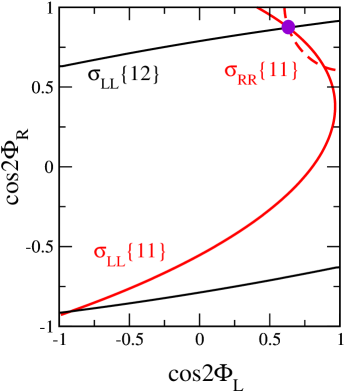
Figure 3: Determining the chargino mixing angles in measurements of chargino production cross sections {ij} for polarized beams.

Based on this high-precision information, the fundamental SUSY parameters can be extracted at low energy in analytic form. To lowest order:

$$\left|\mu\right| = M_{W}[\Sigma+\Delta[\cos 2\phi_{R}+\cos 2\phi_{L}]]^{1/2}$$

$$\mbox{sign}(\mu) = [\Delta^{2}-(M^{2}_{2}-\mu^{2})^{2}-4m^{2}_{W}(M^{2}_{2}+\mu^{2})$$

$$-4m^{4}_{W}\cos^{2}2\beta]/8m_{W}^{2}M_{2}|\mu|\sin 2\beta$$

$$M_{2} = M_{W}[\Sigma-\Delta(\cos 2\phi_{R}+\cos 2\phi_{L})]^{1/2}$$

$$|M_{1}| = \left[\textstyle\sum_{i}m^{2}_{\tilde{\chi}_{i}^{0}}-M^{2}_{2}-\mu^{2}-2M^{2}_{Z}\right]^{1/2}$$

$$|M_{3}| = m_{\tilde{g}}$$

$$\tan\beta = \left[\frac{1+\Delta(\cos 2\phi_{R}-\cos 2\phi_{L})}{1-\Delta(\cos 2\phi_{R}-\cos 2\phi_{L})}\right]^{1/2}$$ (1)

where $\Delta=(m^{2}_{\tilde{\chi}^{\pm}_{2}}-m^{2}_{\tilde{\chi}^{\pm}_{1}})/(4M^{2}_{W})$ and $\Sigma=(m^{2}_{\tilde{\chi}^{\pm}_{2}}+m^{2}_{\tilde{\chi}^{\pm}_{1}})/(2M^{2}_{W})-1$. The signs of $M_{1,3}$ with respect to $M_{2}$ will follow from measurements of the cross sections for ${\tilde{\chi}}{\tilde{\chi}}$ production and gluino processes. In practice one-loop corrections to the mass relations have been used to improve on the accuracy.

Accuracies expected for the parameters in the reference point mod.SPS#1A are shown in Tab. 2. While the LC based errors are typically at the per-mille level, the others turn out to be in the per-cent range.

	Exp. Input	GUT Value
$M_{1}$	102.31 $\pm$ 0.25	$250.00\pm 0.33$
$M_{2}$	192.24 $\pm$ 0.48	$250.00\pm 0.52$
$M_{3}$	0586 $\pm$ 12	$250.0\pm 5.3$
$\mu$	358.23 $\pm$ 0.28	$355.6\pm 1.2$
$M^{2}_{L_{1}}$	$(6.768\pm 0.005)\cdot 10^{4}$	$(3.99\pm 0.41)\cdot 10^{4}$
$M^{2}_{E_{1}}$	$(4.835\pm 0.007)\cdot 10^{4}$	$(4.02\pm 0.82)\cdot 10^{4}$
$M^{2}_{Q_{1}}$	$(3.27\pm 0.08)\cdot 10^{5}$	$(3.9\pm 1.5)\cdot 10^{4}$
$M^{2}_{U_{1}}$	$(3.05\pm 0.11)\cdot 10^{5}$	$(3.9\pm 1.9)\cdot 10^{4}$
$M^{2}_{H_{1}}$	$\phantom{-}(6.21\pm 0.08)\cdot 10^{4}$	$(4.01\pm 0.54)\cdot 10^{4}$
$M^{2}_{H_{2}}$	$(-1.298\pm 0.004)\cdot 10^{5}$	$(4.1\pm 3.2)\cdot 10^{4}$
$A_{t}$	$-446\pm 14\phantom{0\cdot 10^{4}}$	$-100\pm 54\phantom{-0\cdot 10^{4}}$
$\tan\beta$	$\phantom{-}9.9\pm 0.9\phantom{\rule{0.0pt}{0.0pt}\cdot 10^{4}}$	—

Table 2: Reconstructed gaugino and scalar mass parameters for mod.SPS#1A at the electroweak scale and RG extrapolation to the GUT scale; all masses in GeV.

It should be noted that knowledge of the low chargino/neutralino spectrum ${\tilde{\chi}^{\pm}_{1}}$ and $\tilde{\chi}^{0}_{1,2}$ is sufficient to carry out such an analysis. On the other hand, Higgs couplings or polarization effects must be used in addition to determine the Higgs parameter $\tan\beta$ for large values with sufficient accuracy.

The evolution to the high scale is governed by solutions of the renormalization group equations [16]:

gauge couplings	:	$\alpha_{i}=Z_{i}\,\alpha_{U}$
gaugino masses	:	$M_{i}=Z_{i}\,M_{1/2}$
scalar masses	:	$M^{2}_{\tilde{j}}=M^{2}_{0}+c_{j}M^{2}_{1/2}$
		$\phantom{M^{2}_{\tilde{j}}=}+\sum_{\beta=1}^{2}c^{\prime}_{j\beta}\Delta M^{2}_{\beta}$
trilinear couplings	:	$A_{k}=d_{k}A_{0}+d^{\prime}_{k}M_{1/2}$

The $Z$ transporter is given by $Z_{i}^{-1}=1+b_{i}\,\alpha_{U}/(4\pi)$ $\times\log(M_{U}/M_{Z})^{2}$ with $b[SU_{3},SU_{2},U_{1}]=-3$, 1, $33/5$. The $c$, $d$ coefficients as well as the shifts $\Delta M^{2}_{\beta}$ depend on the high-energy parameters to be calculated, so that complicated implicit equations emerge – partly with solutions of low sensitivity. In practice the transport equations have been solved to two loops.

Examples for the gaugino masses and the scalar masses of the first two generations are depicted in Fig. 4. Moving down from the universality point, the mass squared of the Higgs field $H_{2}$ crosses to negative values at a scale of order $10^{4}$ TeV, in accordance with radiative symmetry breaking in mSUGRA.

a)    $1/M_{i}$ [GeV^-1]

Figure 4: mSUGRA: Evolution, from low to high scales, of a) gaugino mass parameters, b) first-generation sfermion mass parameters squared and the Higgs mass parameter $M^{2}_{H_{2}}$. The mSUGRA point probed is defined in Tab. 1. [The widths of the bands indicate the 1$\sigma$ CL.]

	Ideal	Exp. Error
$M_{U}$	$2\cdot 10^{16}$	$1.6\cdot 10^{14}$
$\alpha_{U}^{-1}$	24.361	0.007
$M_{\frac{1}{2}}$	250	0.08
$M_{0}$	200	0.09
$A_{0}$	-100	1.8
$\mu$	358.23	0.21
$\tan\beta$	10	0.1

Table 3: Comparison of the ideal parameters with the experimental expectations for the particular mSUGRA reference point analyzed in this report; all mass parameters are given in units of $GeV$.

In an overall-fit, based on the universality hypothesis per se, we observe accuracies of order per-mille in the gaugino sector while being order per-cent in the scalar sector, cf. Tab. 3.

Left-Right SUGRA: The universal SUGRA model can readily be extended to a left-right symmetric theory [as suggested by non-zero neutrino masses] if the SO(10) unification scale is located in between the SU(5) and the Planck scale. The first and second generation are not changed. Owing to the enhanced Yukawa coupling, the seesaw scale above $10^{10}$ GeV however is felt in the evolution of the third generation – albeit with weak sensitivity. This effect is evident from Fig. 5 in which the evolution of the sfermion mass parameters including the right-handed neutrino sector is compared with the evolution if this sector is cut off.

Figure 5: LR-SUGRA with $\nu_{R}$: Evolution of third-generation slepton mass parameters and the Higgs mass parameter $M_{H_{2}}^{2}$. The mSUGRA point probed is characterized by the same parameters as before while the $\nu_{R_{3}}$ scale is taken close to $10^{14}$ GeV.

mSUGRA vs. GMSB: In gauge mediated supersymmetry breaking GMSB [8] the system is characterized by two scales, defined by the vacuum expectation values of components of the superfield $S$ inducing the symmetry breakdown in the secluded sector. They are related to the masses of the messengers which transport the breaking of SUSY from the secluded sector to the eigen-world [$M_{M}\sim$ PeV within wide margins], and the mass scale $\Lambda$ setting the size of the gaugino and scalar masses. Modulo threshold factors, the gaugino masses $M_{i}$ and the scalar masses $M_{\tilde{j}}$, generated by messenger and gauge field induced loops, can be written in compact form,

$$M_{i}(M_{M}) \approx N_{M}\,\alpha_{i}(M_{M})\,\Lambda$$ (2)

$$M_{\tilde{\jmath}}^{2}(M_{M}) \approx 2N_{M}\sum_{i=1}^{3}k_{i}\,C^{j}_{i}\,\alpha_{i}^{2}(M_{M})\,\Lambda^{2}$$ (3)

with $N_{M}$ denoting the multiplicity of messenger multiplets, $k_{i}$ and $C_{i}^{j}$ being group factors, and the $\alpha_{i}$’s are the three gauge couplings. Ratios of scalar masses, $M^{2}_{\tilde{\jmath}}(M_{M})/$ $M^{2}_{\tilde{\jmath}^{\prime}}(M_{M})$ depend only on group factors and gauge couplings so that they can be predicted uniquely in GMSB.

Figure 6: GMSB: Evolution of first-generation slepton mass parameters and Higgs mass parameters $M_{H_{2}}^{2}$. The point probed, SPS#8 is characterized by the parameters $M_{M}=200$ TeV, $\Lambda=100$ TeV, $\tan\beta=15$, and $\rm sign(\mu)=(+)$. [The widths of the bands indicate the 1$\sigma$ CL.]

The evolution of the scalar mass parameters is shown in Fig. 6. The bands of the slepton $\tilde{L}$-doublet and the second Higgs doublet $H_{2}$, which carry the same moduli of standard-model charges, cross at the scale $M_{M}$. The two scales $M_{M}$ and $\Lambda$, and the messenger multiplicity $N_{M}$ can be extracted from the spectrum of the gaugino and scalar particles. For the reference point analyzed in the Fig. 6, the following accuracies can be obtained:

$$\Lambda = (1.01\pm 0.03)\cdot 10^{2}{\rm\ TeV}$$

$$M_{M} = (1.92\pm 0.24)\cdot 10^{2}{\rm\ TeV}$$

$$N_{M} = 0.978\pm 0.056$$

Comparing the two figures representative for the evolution of the scalar mass parameters, it is manifest that mSUGRA will not be confused with GMSB so long as the messenger scale does not move out of the PeV range to the Planck scale – which would be a contradictio in origine.

3 String Effective Field Theory

Among the most exciting candidates for a comprehensive theory of matter and interactions rank superstring theories. We will summarize results obtained for a string effective field theory in four dimensions based on orbifold compactification of the 10-dimensional heterotic superstring [5]. SUSY breaking is generated non-perturbatively in this approach, mediated by a Goldstino field that is the superposition of the dilaton field $S$ and the moduli fields $T$ [all moduli fields assumed to be of identical structure]:

$$G=S\sin\theta+T\cos\theta$$ (4)

Universality is generally broken in such a scenario by a set of non-universal modular weights $n_{j}$ that determine the coupling of $T$ to the SUSY matter fields $\Phi_{j}$.

The gaugino and scalar mass parameters can be expressed to leading order by the gravitino mass $m_{3/2}$, the vacuum value $\langle S\rangle$, the mixing parameter $\sin\theta$, and the modular weights $n_{j}$:

$$M_{i} = -g_{i}^{2}m_{3/2}{\langle S\rangle}{\sqrt{3}\sin\theta}+\cdots$$

$$M_{\tilde{j}}^{2} = m^{2}_{3/2}\left(1+n_{j}\cos^{2}\theta\right)+\cdots$$ (5)

while in next-to-leading order, indicated by the ellipses, the vacuum value $\langle T\rangle$ and the Green-Schwarz parameter $\delta_{\rm GS}$ are included. The system is completed by relations between the universal gauge coupling $\alpha(M_{\rm string})$ at the string scale $M_{\rm string}$ and the [slightly non-universal] gauge couplings $\alpha_{i}(M_{\rm GUT})$ at the SU(5) unification scale $M_{\rm GUT}$:

$$\alpha^{-1}_{i}(\rm M_{\rm GUT})=\alpha^{-1}({\rm M_{\rm string}})+\Delta\alpha^{-1}_{i}[n_{j}]$$ (6)

The small deviations of the gauge couplings from universality at the GUT scale are accounted for by string loop effects transporting the couplings from the universal string scale to the GUT scale. The gauge coupling at $M_{\rm string}$ is related to the dilaton field, $g_{s}^{2}=1/{\langle S\rangle}$.

Figure 7: String Scenario: Gaugino mass parameters for the heterotic string [the insert expands on the breaking of universality at the GUT scale]. The point probed is characterized by the parameters $m_{3/2}=180$ GeV, $\delta_{GS}=0$, $\langle S\rangle=2$, $\langle T\rangle=14\,m_{3/2}$, $\sin^{2}\theta=0.9$, $\tan\beta=10$, $\mathrm{sign}(M_{2}\mu)=(+)$, $n_{L_{i}}=-3$, $n_{E_{i}}=-1$, $n_{H_{1}}=n_{H_{2}}=-1$, $n_{Q_{i}}=0$, $n_{D_{i}}=1$ and $n_{U_{i}}=-2$. [The widths of the bands indicate the $1\,\sigma$ CL.]

Parameter	Ideal	Reconstructed
$m_{3/2}$	180	179.9	$\pm$	0.4
$\langle S\rangle$	2	1.998	$\pm$	0.006
$\langle T\rangle/m_{3/2}$	14	14.6	$\pm$	0.2
$\sin\theta$	0.949	0.948	$\pm$	0.001
$g_{s}^{2}$	0.5	0.501	$\pm$	0.002
$\delta_{GS}$	0	0.1	$\pm$	0.4
$n_{L}$	-3	-2.94	$\pm$	0.04
$n_{E}$	-1	-1.00	$\pm$	0.05
$n_{Q}$	0	0.02	$\pm$	0.02
$n_{U}$	-2	-2.01	$\pm$	0.02
$n_{D}$	+1	0.80	$\pm$	0.04
$n_{H_{1}}$	-1	-0.96	$\pm$	0.06
$n_{H_{2}}$	-1	-1.00	$\pm$	0.02
$\tan\beta$	10	10.00	$\pm$	0.13

Table 4: Comparison of the experimentally reconstructed values with the ideal fundamental parameters in a specific example for a string effective field theory; masses in GeV.

The evolution of the gaugino masses in such a scenario is illustrated in Fig. 7, with the crucial high-scale region expanded in the insert. Relevant parameters constructed from an overall-fit to couplings and masses are collected in Tab. 4. It turns out that the ideal values, from which the experimental input observables were derived, can indeed be extracted from the data collected at high-energy hadron- and lepton-colliders that will allow to perform the high-precision measurements required for this purpose.

4 Conclusions

In this summary report we have demonstrated that, based on future high-precision data from e⁺e^- linear colliders, TESLA in particular, and combined with results from LHC, and later CLIC, the fundamental supersymmetry parameters can be reconstructed at the high scale, GUT or Planck, in practice. The bottom-up approach of evolving the parameters from the low-energy scale to the high scale by means of renormalization group techniques provides us with a transparent picture in a region where gravity is linked to particle physics, and superstring theory becomes effective directly. We have exemplified this – truly exciting – observation in two ways explicitly, for minimal supergravity theories, and for a string effective field theory based on orbifold compactification of the heterotic string. We could demonstrate that the effective string parameters can indeed be reconstructed from high-precision high-energy experiments at hadron- and lepton-colliders.

Acknowledgements: This work was supported in part by the European Commision 5th framework under contract HPRN-CT-2000-00149 and the Polish-German LC project No. POL 00/015. W. P. is supported by the ”Erwin Schrödinger fellowship No. J2095” of the ”Fonds zur Förderung der wissenschaftlichen Forschung” of Austria FWF and partly by the Swiss ”Nationalfonds”.

References

- [1] J. Wess and B. Zumino, Nucl. Phys. B 70 (1974) 39.
- [2] H.P. Nilles, Phys. Rept. 110 (1984) 1; H.E. Haber and G.L. Kane, Phys. Rept. 117 (1985) 75.
- [3] E. Witten, Nucl. Phys. B 188 (1981) 513.
- [4] A.H. Chamseddine, R. Arnowitt, and P. Nath, Phys. Rev. Lett. 49 (1982) 970.
- [5] M. Cvetič, A. Font, L.E. Ibáñez, D. Lüst and F. Quevedo, Nucl. Phys. B 361 (1991) 194; A. Brignole, L.E. Ibáñez and C. Muñoz, Nucl. Phys. B 422 (1994) 125 [Erratum-ibid. B 436 (1995) 747]; A. Love and P. Stadler, Nucl. Phys. B 515 (1998) 34; P. Binetruy, M.K. Gaillard and B.D. Nelson, Nucl. Phys. B 604 (2001) 32.
- [6] G.A. Blair, W. Porod and P.M. Zerwas, Phys. Rev. D 63 (2001) 017703; cont’d in DESY 02-166 and hep-ph/0210058.
- [7] G.L. Kane, Proceedings SUSY02, Hamburg 2002, and hep-ph/0210352.
- [8] M. Dine and A. E. Nelson, Phys. Rev. D 48 (1993) 1277.
- [9] E. Accomando et al., ECFA/DESY LC Working Group, Phys. Rep. 299 (1998) 1; “TESLA Technical Design Report Part III: Physics at an e+e- Linear Collider”, eds. R. Heuer, D.J. Miller, F. Richard and P.M. Zerwas, DESY 01-011 and hep-ph/0106315.
- [10] T. Behnke, J.D. Wells and P.M. Zerwas, Prog. Part. Nucl. Phys. 48 (2002) 363.
- [11] J.L. Feng and M.N. Nojiri, Report UCI-TR-2002 -25 and hep-p/0210390.
- [12] B.C. Allanach et al., in Proc. of the APS/DPF/DPB Summer Study on the Future of Particle Physics (Snowmass 2001) ed. R. Davidson and C. Quigg, hep-ph/0202233, and Eur. Phys. J. C 25 (2002) 113.
- [13] G.A. Blair and U. Martyn, Proceedings, LC Workshop, Sitges 1999, hep-ph/9910416.
- [14] S.Y. Choi, A. Djouadi, M. Guchait, J. Kalinowski, H.S. Song and P.M. Zerwas, Eur. Phys. J. C 14 (2000) 535; S.Y. Choi, J. Kalinowski, G. Moortgat-Pick and P.M. Zerwas, Eur. Phys. J. C 22 (2001) 563 [Addendum-ibid. C 23 (2002) 769].
- [15] A. Freitas et al., Proceedings ICHEP.2002, Amsterdam 2002.
- [16] S. Martin and M. Vaughn, Phys. Rev. D50, 2282 (1994); Y. Yamada, Phys. Rev. D 50, 3537 (1994); I. Jack, D.R.T. Jones, Phys. Lett. B 333 (1994) 372.