Current in the light-front Bethe-Salpeter formalism II:
Applications

Abstract

We pursue applications of the light-front reduction of current matrix elements in the Bethe-Salpeter formalism. The normalization of the reduced wave function is derived from the covariant framework and related to non-valence probabilities using familiar Fock space projection operators. Using a simple model, we obtain expressions for generalized parton distributions that are continuous. The non-vanishing of these distributions at the crossover between kinematic regimes (where the plus component of the struck quark’s momentum is equal to the plus component of the momentum transfer) is tied to higher Fock components. Moreover continuity holds due to relations between Fock components at vanishing plus momentum. Lastly we apply the light-front reduction to time-like form factors and derive expressions for the generalized distribution amplitudes in this model.

I Introduction

More than a half century ago, Dirac’s paper on the forms of relativistic dynamics Dirac:1949cp introduced the front-form Hamiltonian approach. Applications to quantum mechanics and field theory were overlooked at the time due to the appearance of covariant perturbation theory. The reemergence of front-form dynamics was largely motivated by simplicity as well as physicality. The light-front approach has the largest stability group Leutwyler:1977vy of any Hamiltonian theory. Today the physical connection to light-front dynamics is transparent: hard scattering processes probe a light-cone correlation of the fields. Not surprisingly, then, many perturbative QCD applications can be treated on the light front, see e.g. Lepage:1980fj . Outside this realm, physics on the light cone has been extensively developed for non-perturbative QCD Brodsky:1997de as well as applied to nuclear physics Carbonell:1998rj ; Miller:2000kv .

Recently we investigated current matrix elements in the light-front Bethe-Salpeter formalism future , at task originally attempted in Tiburzi:2002mn . As an example, we considered the ladder approximation for the covariant kernel in the weak-binding limit. We calculated $(1+1)$-dimensional electromagnetic form factors in this reduction scheme to demonstrate the replacement of non-wave function vertices (as coined in Bakker:2000rd ) with contributions from higher Fock states. These higher Fock states originate from the light-front energy pole-structure of the Bethe-Salpeter and photon vertices.

Below, we take the model into $(3+1)$ dimensions and make clear the connection to higher Fock components by explicitly constructing the three-body wave function from our expressions for form factors. Additionally we show how the normalization of the covariant Bethe-Salpeter equation turns into a familiar many-body normalization in the light-front reduction. The immediate application of our development for form factors (in a frame where the plus-component of the momentum transfer is non-zero) is to compute generalized parton distributions. Connection is again made to the Fock space representation and continuity of the distributions is put under scrutiny. The formalism is also employed to obtain time-like form factors. This latter application in interesting since no Fock space expansion in terms of bound states is possible.

The paper is organized as follows. First in section II we review the normalization of the covariant Bethe-Salpeter wave function and then proceed to derive the light-front reduced version. This necessitates a review of the light-front reduction notation introduced in Sales:1999ec . The normalization condition resembles a diagonal matrix element of a pseudo current and has contributions from higher Fock states. We calculate the explicit normalization condition for the ladder model at next-to-leading order in perturbation theory. The connection to the familiar many-body Fock state normalization is made in Appendix B. Next in section III, we use the reduction scheme to calculate generalized parton distributions. We do so by using the integrand of the electromagnetic form factor calculated in an arbitrary frame (these expressions in $(3+1)$ dimensions are collected in Appendix A where the leading-order bound-state equation for the wave function also appears). We discuss the continuity of these distributions in terms of relations between Fock components at vanishing plus momentum. Connection is also made to the overlap representation of generalized parton distributions. Application of the reduction scheme to time-like form factors and their related generalized distribution amplitudes is presented in section IV. Finally we conclude with a brief summary (section V).

II Normalization

In Sales:1999ec the relation between the four-dimensional Bethe-Salpeter wave function and the reduced light-front wave function was presented. The normalization of the reduced wave function, however, was not discussed in much detail and will be addressed below.

Let $G(R)$ denote the two-particle disconnected propagator, where $R$ labels the total momentum. Thus between effective single-particle states of momenta $p$ and $k$, we have $\langle p|G(R)|k\rangle=(2\pi)^{4}\delta^{4}(p-k)G(k,R)$, where $G(k,R)=d(k)d(R-k)$ and the scalar single-particle propagator is

$$d(k)=\frac{i}{(k^{2}-m^{2})[1+(k^{2}-m^{2})f(k^{2})]+\operatorname{i\epsilon}}.$$ (1)

Here the function $f(k^{2})$ characterizes the renormalized, one-particle irreducible self-interactions and for simplicity shall be ignored below. The Bethe-Salpeter equation for the bound-state amplitude $|\Psi_{R}\rangle$ with mass $R^{2}=M^{2}$ reads

$$|\Psi_{R}\rangle=G(R)V(R)|\Psi_{R}\rangle,$$ (2)

where $V(R)$ is the irreducible two-to-two scattering kernel (which we shall often call the potential).

From the behavior of the reducible four-point function near the bound-state pole $R^{2}=M^{2}$ one can deduce the covariant normalization condition Itzykson:rh by application of l’Hôpital’s rule

$$2iR^{\mu}=\langle\Psi_{R}|\frac{\partial}{\partial R_{\mu}}\Big{(}G^{-1}(R)-V(R)\Big{)}|\Psi_{R}\rangle\;\Bigg{|}_{R^{2}=M^{2}}.$$ (3)

The normalization (3) takes the form of a diagonal matrix element of a pseudo current.

The light-front reduction is performed by integrating out the minus-momentum dependence with the help of an auxiliary Green’s function $\operatorname{\tilde{G}}(R)$. For simplicity, we denote the integration $\int\frac{d\operatorname{k^{--}}}{2\pi}\langle\operatorname{k^{--}}|\mathcal{O}(R)=\Big{|}\mathcal{O}(R)$. With this notation, we will always work in $(3+1)$-dimensional momentum space for which the only sensible matrix elements of $\Big{|}\mathcal{O}(R)$ are of the form $\langle\operatorname{k^{+}},\operatorname{\mathbf{k}^{\perp}}|\;\Big{|}\mathcal{O}(R)|\operatorname{p^{--}},\operatorname{p^{+}},\operatorname{\mathbf{p}^{\perp}}\rangle$. The operator $\mathcal{O}(R)\Big{|}$ is defined similarly. To obtain light-front time-ordered perturbation theory one chooses

$$\operatorname{\tilde{G}}(R)=G(R)\Big{|}g^{-1}(R)\Big{|}G(R),$$ (4)

where $g(R)=\Big{|}G(R)\Big{|}$. This form of $\operatorname{\tilde{G}}$ allows for a systematic approximation scheme for the light-front energy poles of the Bethe-Salpeter vertex future . Lastly one defines an auxiliary kernel $W(R)$ by Woloshyn:wm

$$W(R)=V(R)+\Big{(}G(R)-\operatorname{\tilde{G}}(R)\Big{)}W(R).$$ (5)

In what follows we shall omit total four-momentum labels since they are all identically $R$. The normalization condition for the reduced wave function is then deduced by using the conversion Sales:1999ec

$$|\Psi_{R}\rangle=\Bigg{(}1+\Big{(}G-\operatorname{\tilde{G}}\Big{)}W\Bigg{)}G\Big{|}\;|\gamma_{R}\rangle,$$ (6)

and the definition of the reduced wave function $|\psi_{R}\rangle$, namely

$$|\psi_{R}\rangle\equiv\Big{|}\;|\Psi_{R}\rangle=g(R)|\gamma_{R}\rangle.$$ (7)

Hence taking the plus component of Eq. (3)

$$2iR^{+}=\langle\gamma_{R}|\;\Big{|}G\Bigg{(}1+W(G-\operatorname{\tilde{G}})\Bigg{)}\\ \times\Bigg{(}\frac{\partial}{\partial R^{-}}\Big{[}G^{-1}-V\Big{]}\Bigg{)}\Bigg{(}1+(G-\operatorname{\tilde{G}})W\Bigg{)}G\Big{|}\;|\gamma_{R}\rangle.$$ (8)

The complicated normalization condition is indicative of the effects of higher Fock space components. To see this explicitly, we work in the ladder model in perturbation theory for which

$$V(k,p)=\frac{-g^{2}}{(k-p)^{2}-\mu^{2}+\operatorname{i\epsilon}}.$$ (9)

Notice $\partial V/\partial R^{\mu}=0$.

Let us start with the contribution at leading order in $G-\operatorname{\tilde{G}}$ to the reduced wave function’s normalization.

$$\frac{-i}{2R^{+}}\langle\gamma_{R}|\;\Big{|}G\Big{(}\frac{\partial}{\partial R^{-}}G^{-1}\Big{)}G\Big{|}\;|\gamma_{R}\rangle=1.$$ (10)

To perform the integration, we note

$$\frac{\partial}{\partial R^{-}}G^{-1}(k,R)=-2iR^{+}d^{-1}(k)(1-x),$$ (11)

where we have customarily chosen $x=\operatorname{k^{+}}/R^{+}$. Evaluation of the integral in equation (10) is standard and yields

$$N^{\text{LO}}\equiv\int\frac{dxd\operatorname{\mathbf{k}^{\perp}}}{2(2\pi)^{3}x(1-x)}\psi^{*}(x,\operatorname{\mathbf{k}^{\perp}})\psi(x,\operatorname{\mathbf{k}^{\perp}})=1,$$ (12)

a simple overlap of the two-body wave function.

To analyze the normalization to first order in $G-\operatorname{\tilde{G}}$, we expand equation (8) to first order

$$N^{\text{LO}}+\delta N+\ldots=1,$$ (13)

where $N^{\text{LO}}$ is the integral appearing in (12) and the first-order correction arising from (8) is

$$\delta N=\frac{-i}{2R^{+}}\langle\gamma_{R}|\;\Big{|}G\Big{(}\frac{\partial}{\partial R^{-}}G^{-1}\Big{)}\Big{(}G-\operatorname{\tilde{G}}\Big{)}VG\\ +GV\Big{(}G-\operatorname{\tilde{G}}\Big{)}\Big{(}\frac{\partial}{\partial R^{-}}G^{-1}\Big{)}G\Big{|}\;|\gamma_{R}\rangle.$$ (14)

The presence of $\operatorname{\tilde{G}}$ merely subtracts the leading-order result $N^{\text{LO}}$. Considering for the moment just the first term in the above equation (and omitting the subtraction $\operatorname{\tilde{G}}$), we have

$$-i\int\frac{d^{4}k}{(2\pi)^{4}}\;\frac{d^{4}p}{(2\pi)^{4}}(1-x)\gamma^{*}(x,\operatorname{\mathbf{k}^{\perp}}|M^{2})d(k)\\ \times d(R-k)^{2}V(k,p)d(p)d(R-p)\gamma(y,\operatorname{\mathbf{p}^{\perp}}|M^{2}).$$ (15)

The minus-momentum integrals above are similar to those considered in deriving the bound-state equation to leading order in Appendix A. The only difference is the double pole due to the extra propagator $d(R-k)$. With $x=\operatorname{k^{+}}/R^{+}$ and $y=\operatorname{p^{+}}/R^{+}$, for $x>y$ we avoid picking up the residue at the double pole and the result is the same as in Eq. (10) after using the bound-state equation. This term is then subtracted by the $\operatorname{\tilde{G}}$ term in equation (14). On the other hand, when $x<y$ we pick up the residue at the double pole. Part of the residue is subtracted by the $\operatorname{\tilde{G}}$ term; the other half depends on $\partial V(k,p)/\partial k^{-}$. The second term in Eq. (14) is evaluated identically up to $\{k\leftrightarrow p\}$. Now combining the two terms and their relevant $\theta$ functions, we can rewrite the result using the explicit form of the one-boson exchange potential Eq. 43, namely

$$\delta N=\int\frac{dxd\operatorname{\mathbf{k}^{\perp}}}{2(2\pi)^{3}x(1-x)}\;\frac{dyd\operatorname{\mathbf{p}^{\perp}}}{2(2\pi)^{3}y(1-y)}\psi^{*}(x,\operatorname{\mathbf{k}^{\perp}})\Bigg{(}-\frac{\partial}{\partial M^{2}}V(x,\operatorname{\mathbf{k}^{\perp}};y,\operatorname{\mathbf{p}^{\perp}}|M^{2})\Bigg{)}\psi(y,\operatorname{\mathbf{p}^{\perp}}).$$ (16)

Thus although the covariant derivative’s action on the potential vanishes, we can manipulate the correction to the normalization into the form of a derivative’s action on the light-front, time-ordered potential. With this form, we can compare to the familiar nonvalence probability discussed in Appendix B (in the frame where $R^{+}=R^{-}=M/\sqrt{2}$ with $M/\sqrt{2}$ as the eigenvalue of the light-front Hamiltonian, denoted $\operatorname{p^{--}}$ in Eq. (65)).

Here we have seen that the normalization of the light-cone wave function includes effects from higher Fock states. Since this normalization condition stemmed from a diagonal matrix element of a pseudo current, we should not be surprised that matrix elements of the electromagnetic current, when treated in this reduction scheme, pick up contributions from higher Fock states. These higher Fock contributions appear explicitly and are the subject of the next section.

III Application to GPDs

Having worked through matrix elements of the electromagnetic current in a frame where $\Delta^{+}\neq 0$ future , we can now make the connection to generalized parton distributions (GPDs). These distributions, which in some sense are the natural interpolating functions between form factors and quark distribution functions, turn up in a variety of hard exclusive processes, e.g. deeply virtual Compton scattering, wide-angle Compton scattering and the electro-production of mesons Muller:1994fv . The scattering amplitude for these processes factorizes into a convolution of a hard part (calculable from perturbative QCD) and a soft part which the GPDs encode. Since light-cone correlations are probed in these hard processes, the soft physics has a simple interpretation and expression in terms of light-front wave functions Brodsky:2001xy . In this section, we cast our results for form factors future in the language of GPDs and the light cone Fock space expansion. The $(3+1)$-dimensional expressions for form factors are presented in Appendix A. Additionally one can obtain these results directly from time-ordered perturbation theory using two-body projection operators as explicated in Appendix B.

The GPD for our meson model is defined by a non-diagonal matrix element of bilocal field operators

$$F(x,\zeta,t)=\int\frac{dy^{-}}{4\pi}e^{ixP^{+}y^{-}}\langle\Psi_{P^{\prime}}|\;q(y^{-})i\overset{\leftrightarrow}{\partial}{}^{+}q(0)\;|\Psi_{P}\rangle,$$ (17)

where $q(x)$ denotes the quark field operator and $\overset{\leftrightarrow}{\partial}{}^{\mu}=\overset{\rightarrow}{\partial}{}^{\mu}-\overset{\leftarrow}{\partial}{}^{\mu}$. Comparing to the current matrix element $J^{\mu}$ in Appendix A, the definition of the GPD leads immediately to the sum rule

$$\int\frac{dx}{1-\zeta/2}F(x,\zeta,t)=F(t).$$ (18)

Hence one can calculate these distributions from the integrand of the form factor. In this way, the light-cone correlation defined in Eq. (17) has a natural description in terms of light-front time-ordered perturbation theory, e.g. for $x>\zeta$ the relevant graphs contributing to the GPD are in Figure 4 and 5, and those for $x<\zeta$ are in Figure 6.

III.1 Continuity

Conversion of the contributions to the form factor into GPDs is straightforward using Eq. (18); we merely remove $-2iP^{+}$ and $\int dx$ from Eqs. (52-57). In order for the deeply virtual Compton scattering amplitude to factorize into hard and soft pieces (at leading twist), the GPDs $F(x,\zeta,t)$ must be continuous at $x=\zeta$. Maintaining continuity at the crossover is more pressing because experiments which measure the beam-spin asymmetry are limited to the crossover Diehl:1997bu . The leading-order expressions are continuous. This is easy to see since the contribution for $x<\zeta$ is identically zero. The valence contribution for $x>\zeta$ is a convolution of wave functions one of which is $\psi^{*}(x^{\prime},\ldots)$ which is probed at the end point since $x^{\prime}\equiv\frac{x-\zeta}{1-\zeta}\to 0$. From the bound-state equation Eq. (45), we see the two-body wave function vanishes quadratically at the end points. Taking into account the overall weight $x^{\prime-1}$, the valence piece vanishes linearly at the crossover. At leading order then, continuity is maintained at the crossover, while the derivative is discontinuous. Working only in the valence sector, valence quark models will never be of any use to beam-spin asymmetry measurements since the value at the crossover requires one wave function to be at an end point. In the three-body bound state problem (e.g. the nucleon), the valence GPD will vanish only if the three-body interaction is non-singular at the end points (which is physically reasonable and perturbatively true).

Let us now check the next-to-leading order contributions to the GPD for continuity. First we shall deal with the term stemming from iterating the Bethe-Salpeter equation for the initial state (55) (see diagram $B$ of Figure 5). Since there is no Z-graph generated from iterating the initial state, we expect this contribution to vanish. Looking at the expression, we see again $\psi^{*}(x^{\prime},\ldots)/x^{\prime}$ which vanishes linearly as $x\to\zeta$. Moreover there are the interaction terms: $D(y,\operatorname{\mathbf{p}^{\perp}};x,\operatorname{\mathbf{k}^{\perp}}|M^{2})$ which is finite as $x\to\zeta$, and

$$D(\operatorname{y^{\prime}},\operatorname{\mathbf{p}^{\prime\perp}};\operatorname{x^{\prime}},\operatorname{\mathbf{k}^{\prime\perp}}|M^{2})\overset{x\to\zeta}{=}\frac{-\operatorname{x^{\prime}}}{(\operatorname{\mathbf{k}^{\perp}}+\mathbf{\Delta}^{\perp})^{2}+m^{2}},$$ (19)

which vanishes at the crossover. Thus not only does the initial-state iteration term vanish at the crossover, its derivative does so as well.

Now we investigate the Born terms 53 (see diagram $A$ of Figure 5) and 54 (see diagram $D$ of Figure 6) at the crossover. Approaching $\zeta$ from above (53), we have the finite contribution at the crossover

$$F(\zeta,\zeta,t)^{\text{Born}}=\int\frac{d\operatorname{\mathbf{k}^{\perp}}dyd\operatorname{\mathbf{p}^{\perp}}}{(16\pi^{3})^{2}y(1-y)\operatorname{y^{\prime}}}\psi^{*}(y^{\prime},\operatorname{\mathbf{p}^{\prime\perp}})\frac{g^{2}\theta(y-\zeta)/(y-\zeta)}{(\operatorname{\mathbf{k}^{\perp}}+\mathbf{\Delta}^{\perp})^{2}+m^{2}}D(y,\operatorname{\mathbf{p}^{\perp}};\zeta,\operatorname{\mathbf{k}^{\perp}}|M^{2})\psi(y,\operatorname{\mathbf{p}^{\perp}}).$$ (20)

On the other hand, approaching the crossover from below (54) we have to deal with singularities as $x^{\prime\prime}=x/\zeta\to 1$. Writing out the propagator for the quark-antiquark pair heading off to annihilation, we see

$$\operatorname{D_{\text{W}}}(x^{\prime\prime},\operatorname{\mathbf{k}^{\prime\prime\perp}}|t)\to-\frac{1-x^{\prime\prime}}{(\operatorname{\mathbf{k}^{\perp}}+\mathbf{\Delta}^{\perp})^{2}+m^{2}}.$$ (21)

This linear vanishing cancels the weight $(1-x^{\prime\prime})^{-1}$. Taking the limit $x\to\zeta$ then produces equation (20) and thus the Born terms are continuous.

Lastly we must see how the final-state iteration terms match up at the crossover. Using Eq. (56) to approach $\zeta$ from above (see diagram $C$ of Figure 5), we have the contribution

$$F(\zeta,\zeta,t)^{\text{final}}=\int\frac{d\operatorname{\mathbf{k}^{\perp}}d\operatorname{y^{\prime}}d\operatorname{\mathbf{p}^{\prime\perp}}}{(16\pi^{3})^{2}(1-\zeta)\operatorname{y^{\prime}}(1-\operatorname{y^{\prime}})}\psi^{*}(y^{\prime},\operatorname{\mathbf{p}^{\prime\perp}})\frac{g^{2}/y}{(\operatorname{\mathbf{k}^{\perp}}+\mathbf{\Delta}^{\perp})^{2}+m^{2}}D(y,\operatorname{\mathbf{p}^{\perp}};\zeta,\operatorname{\mathbf{k}^{\perp}}|M^{2})\psi(\zeta,\operatorname{\mathbf{k}^{\perp}}).$$ (22)

Approaching $\zeta$ from below (see diagram $E$ of Figure 6), we utilize equation (21) in taking the limit of (57). The result is (22) and hence we have demonstrated continuity to first order, i.e.

$$F(\zeta,\zeta,t)=F(\zeta,\zeta,t)^{\text{Born}}+F(\zeta,\zeta,t)^{\text{final}}$$ (23)

no matter how we approach $x=\zeta$.

III.2 Fock space representation

We now write the GPDs in terms of Fock component overlaps. In the diagonal overlap region $x>\zeta$ this will be a mere rewriting of our results, while there is a subtlety for the non-diagonal overlaps. To handle the zeroth-order term (52), we define the two-body Fock component as

$$\psi_{2}(x_{1},\mathbf{k}^{\perp}_{1},x_{2},\mathbf{k}^{\perp}_{2})=\frac{1}{\sqrt{x_{1}x_{2}}}\psi(x_{1},\mathbf{k}^{\perp}_{\text{rel}}),$$ (24)

noting that the relative transverse momentum can be defined as $\mathbf{k}^{\perp}_{\text{rel}}=x_{2}\mathbf{k}^{\perp}_{1}-x_{1}\mathbf{k}^{\perp}_{2}$. In terms of Eq. (24), the GPD appears as

$$F(x,\zeta,t)^{\text{LO}}=\frac{\theta(x-\zeta)}{\sqrt{1-\zeta}}\int[dx]_{2}[d\operatorname{\mathbf{k}^{\perp}}]_{2}\sum_{j=1,2}\delta(x-x_{j})\psi_{2}^{*}(x^{\prime}_{i},\mathbf{k}^{\prime}_{i}{}^{\perp})\frac{2x_{j}-\zeta}{\sqrt{x^{\prime}_{j}x_{j}}}\psi_{2}(x_{i},\mathbf{k}_{i}^{\perp}),$$ (25)

where the primed variables are given by

$$\begin{cases}x^{\prime}_{i}=\frac{x_{i}}{1-\zeta}\\ \mathbf{k}^{\prime}_{i}{}^{\perp}=\mathbf{k}_{i}^{\perp}-x^{\prime}_{i}\mathbf{\Delta}^{\perp},\;\text{for}\;i\neq j\end{cases}\begin{cases}x^{\prime}_{j}=\frac{x_{j}-\zeta}{1-\zeta}\\ \mathbf{k}^{\prime}_{j}{}^{\perp}=\mathbf{k}_{j}^{\perp}+(1-x^{\prime}_{j})\mathbf{\Delta}^{\perp}\end{cases}$$ (26)

and the integration measure is given by

$$[dx]_{N} =\prod_{i=1}^{N}dx_{i}\;\delta\Big{(}1-\sum_{i=1}^{N}x_{i}\Big{)}$$ (27)

$$[d\operatorname{\mathbf{k}^{\perp}}]_{N} =\frac{1}{[2(2\pi)^{3}]^{N-1}}\prod_{i=1}^{N}d\mathbf{k}^{\perp}_{i}\;\delta\Big{(}\sum_{i=1}^{N}\mathbf{k}^{\perp}_{i}\Big{)}.$$ (28)

Notice the sum over transverse momenta in the delta function is zero since our initial meson has $\mathbf{P}^{\perp}=0$. The sum over $j$ in Eq. (25) produces the overall factor of two for our case of equally massive (equally charged) constituents.

To cast the next-to-leading order expressions for $x>\zeta$ in terms of diagonal Fock space overlaps, we must write out the three-body Fock component. Looking at the diagrams in Figure 5, it is constructed from the two-body wave function

$$\psi_{3}(x_{i},\mathbf{k}_{i}^{\perp})=g\frac{2(2\pi)^{3}}{\sqrt{x_{1}x_{2}x_{3}}}\int[dy]_{2}[d\operatorname{\mathbf{p}^{\perp}}]_{2}\Bigg{[}\theta(y_{1}-x_{1})x_{3}\delta(y_{2}-x_{3})\delta(\mathbf{p}^{\perp}_{2}-\mathbf{k}^{\perp}_{3})D(y_{1},\mathbf{p}^{\perp}_{1};x_{1},\mathbf{k}^{\perp}_{1}|M^{2})\\ +\theta(y_{2}-x_{3})x_{1}\delta(y_{1}-x_{1})\delta(\mathbf{p}^{\perp}_{1}-\mathbf{k}^{\perp}_{1})D(y_{2},\mathbf{p}^{\perp}_{2};x_{3},\mathbf{k}^{\perp}_{3}|M^{2})\Bigg{]}\frac{\psi_{2}(y_{j},\mathbf{p}_{j}^{\perp})}{\sqrt{y_{1}y_{2}}},$$ (29)

where $i$ runs from one to three and the label $j$, which stems from the integration measure, runs from one to two. We discuss how to obtain this three-body wave function directly from time-ordered perturbation theory in Appendix B. Using $\psi_{3}$ in Eq. (29), the terms in the GPD at first order in the weak coupling can then be written compactly as

$$F(x,\zeta,t)^{\text{NLO}}=\frac{\theta(x-\zeta)}{1-\zeta}\int[dx]_{3}[d\operatorname{\mathbf{k}^{\perp}}]_{3}\sum_{j=1,3}\delta(x-x_{j})\psi_{3}^{*}(x_{i}^{\prime},\mathbf{k}_{i}^{\prime}{}^{\perp})\frac{2x_{j}-\zeta}{\sqrt{x^{\prime}_{j}x_{j}}}\psi_{3}(x_{i},\mathbf{k}^{\perp}_{i}).$$ (30)

One can verify that the diagrams in Figure 5 are generated by (30). Additionally there is a fourth diagram generated by Eq. (30) which does not appear in the figure. This missing diagram is characterized by the spectator quark’s one-loop self interaction and is absent since we have ignored $f(k^{2})$ and the scale dependence of light-cone wave functions. The absence of this diagram does not affect continuity at the crossover. The missing diagram vanishes at $x=\zeta$ since the final-state wave function is $\psi^{*}(x^{\prime},\ldots)$. Lastly we note the above Fock component overlaps satisfy the positivity constraint for a composite scalar composed of scalar constituents Tiburzi:2002kr .

Now we must come to terms with the non-diagonal overlap region, $x<\zeta$. At first order, the diagrams of Figure 6 correspond to four-to-two Fock component overlaps. We have been cavalier about time ordering, however. The expressions Eqs. 54 and 57 do not correspond to time-ordered graphs. Both terms contain a product of time-ordered propagators: one for the two quarks leading to the final-state vertex and another for the quark-antiquark pair heading off to annihilation. But for an interpretation in terms of a four-body wave function, all four particles must propagate at the same time. This is a subtle issue as a graph containing the product of two independently time-ordered pieces (where one leads to a bound-state vertex) corresponds to a sum of infinitely many time-ordered graphs. It is easiest to write out the terms of concern in terms of the propagators’ poles. The quark, anti-quark heading to annihilation have propagators $d(k)$ and $d(k+\Delta)$ and poles we label $k^{-}_{a}$ and $k^{-}_{c}$, respectively. The remaining propagators of interest $d(p^{\prime})$ and $d(P^{\prime}-p^{\prime})$ have poles $p^{-}_{a}$ and $p^{-}_{b}$, respectively. We can then manipulate as follows

$$\frac{1}{k^{-}_{c}-k^{-}_{a}}\;\frac{1}{p^{-}_{b}-p^{-}_{a}}\\ =\frac{1}{p^{-}_{b}-p^{-}_{a}+k^{-}_{c}-k^{-}_{a}}\;\Bigg{(}\frac{1}{p^{-}_{b}-p^{-}_{a}}+\frac{1}{k^{-}_{c}-k^{-}_{a}}\Bigg{)}.$$ (31)

In this form, we have produced the correct energy denominator for the instant of light-front time where four particles are propagating. Multiplying this denominator by the three-body wave function yields the four-body wave function (up to constants). This is the part of the four-body wave function relevant for GPDs (there are additional pieces for two-quark, two-boson states, see Appendix B). In the resulting sum (31), the first term will produce the two-body wave function for the final state and we will have a genuine four-to-two overlap. We do not write this out explicitly.

The second term in Eq. (31), however, contains again the propagator for the pair heading to annihilation. Using the light-front Bethe-Salpeter equation for the vertex (which contains infinitely many times) we can introduce a factor of the time-ordered interaction. The resulting product of independent time orderings can again be manipulated as in Eq. (31). The result produces another overall four-body denominator which contributes to the four-body Fock component of the initial state. Since we iterated the interaction, however, this new contribution is no longer at leading order and can be neglected. Thus the second term in (31) does not contribute at this order.

Having manipulated the GPDs into non-diagonal overlaps for $x<\zeta$, we must wonder if continuity at the crossover is still maintained. In the limit $x\to\zeta$ the light-front energy of the struck quark goes to infinity. Consequently $k^{-}_{c}$, which contains this on shell energy, is infinite and dominates the four-body energy denominator. This is identical to the reasoning in Eqs. 54 and 57 where instead of the four-body denominator, we have $\operatorname{D_{\text{W}}}(x^{\prime\prime},\operatorname{\mathbf{k}^{\perp}}+x^{\prime\prime}\mathbf{\Delta}^{\perp}|t)$ which is dominated by $k^{-}_{c}$ at the crossover. Either way, we arrive at the expressions found above for the crossover (20) and (22).

Having cast our expressions for generalized parton distributions in terms of the Fock components, we can enlarge our understanding of the sum rule and continuity at the crossover. Both must deal with the relation between higher Fock components. The way $\zeta$-dependence disappears from (18) mandates a relation between the diagonal and non-diagonal Fock component overlaps that make up the GPD. The relation between Fock components must follow from the field-theoretic equations of motion. Continuity itself is a special case of the relation between Fock components, specifically at the end points. Above we have seen our expressions are continuous (and non-vanishing) at the crossover and explicitly that the three- and four-body components match at the end point (where $x-\zeta=0$). This weak binding model for behavior at the crossover is a simple example of the relations between Fock components at the end points (see also Antonuccio:1997tw ). More general relations must be permitted from the equations of motion to guarantee Lorentz covariance (e.g. in the structure of the Mellin moments of the GPDs, of which the sum rule is a special case). Here, of course, Lorentz symmetry is broken. Infinitely many light-cone time-ordered graphs are needed in the reduced kernel to reproduce the covariant one-boson exchange (9). Thus exactly satisfying polynomiality requires not only infinitely many exchanges in the kernel but contributions from infinitely many Fock components. It should be possible, however, to show how the sum rule and polynomiality are improved order by order.

IV Application to GDAs

Below we study time-like form factors to demonstrate the versatility of this approach and make the connection to the generalized distribution amplitudes (GDAs) for this model. Analogous to GPDs, GDAs encode the soft physics of two-meson production and can thus be thought of as crossed versions of the GPDs. The GDAs enter in convolutions for various two-meson production amplitudes Diehl:1998dk . These distribution functions as well as time-like form factors are a theoretical challenge for light-front dynamics, since there is no direct decomposition in terms of meson Fock components alone. Furthermore, we shall see the leading-order expressions are non-valence contributions (which necessarily excludes a description in terms of most constituent quark models).

Figure 1: The triangle diagram for the time-like, pion form factor

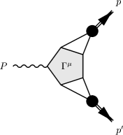
The time-like form factor $F(s)$ for our model meson is defined by (see Figure 1)

$$\langle\Psi_{p}\;\Psi_{p^{\prime}}|\;\Gamma^{\mu}\;|0\rangle=-i(p-p^{\prime})^{\mu}F(s),$$ (32)

where $s=(p+\operatorname{p^{\prime}})^{2}$ is the center of mass energy squared. Now define $P^{\mu}=p^{\mu}+\operatorname{p^{\prime}}{}^{\mu}$ and $\zeta=\operatorname{p^{+}}/\operatorname{P^{+}}$. We can work out the kinematics of this reaction in a frame where $\mathbf{P}^{\perp}=0$

$$P^{-} =\frac{s}{2P^{+}}$$

$$p^{-} =\frac{(1-\zeta)s}{2\operatorname{P^{+}}}$$

$$\mathbf{p}^{\perp}{}^{2} =s(1-\zeta)\zeta-M^{2},$$ (33)

where $M$ is the meson mass.

Similar to GPDs, the GDA for our model has a definition in terms of a non-diagonal matrix element of bilocal field operators

$$\operatorname{\Phi(z,\zeta,s)}=\int\frac{dx^{-}}{2\pi}e^{iz\operatorname{P^{+}}x^{-}}\langle\Psi_{p}\;\Psi_{\operatorname{p^{\prime}}}|\;q(x^{-})i\ \overset{\leftrightarrow}{\partial}{}^{+}q(0)\;|0\rangle.$$ (34)

Such a definition of the GDA leads directly to a sum rule for the time-like form factor

$$\int\frac{dz}{2\zeta-1}\operatorname{\Phi(z,\zeta,s)}=F(s),$$ (35)

and hence a means to calculate $\Phi$ from the integrand of the time-like form factor.

Taking the appropriate residues of the five-point function, we arrive at Fig. 1 for the time-like form factor. Keeping only the leading order piece of the electromagnetic vertex $\Gamma^{\mu}$, we have

$$\operatorname{\Phi(z,\zeta,s)}=i\operatorname{P^{+}}(2z-1)\int\frac{d\operatorname{k^{--}}d\operatorname{\mathbf{k}^{\perp}}}{(2\pi)^{4}}\\ \times\gamma^{*}(\operatorname{z^{\prime\prime}},\operatorname{\mathbf{k}^{\perp}}-\operatorname{z^{\prime\prime}}\operatorname{\mathbf{p}^{\perp}}|M^{2})G(k,p)d^{-1}(k-p)\\ \times G(P-k,\operatorname{p^{\prime}})\gamma^{*}\big{(}\operatorname{z^{\prime}},\operatorname{\mathbf{k}^{\perp}}-(1-\operatorname{z^{\prime}})\operatorname{\mathbf{p}^{\perp}}\big{|}M^{2}\big{)},$$ (36)

where we have made use of $z=\operatorname{k^{+}}/\operatorname{P^{+}}$, $\operatorname{z^{\prime}}=\frac{z-\zeta}{1-\zeta}$ and $\operatorname{z^{\prime\prime}}=z/\zeta$. Recall $\gamma(x|M^{2})\propto\theta[x(1-x)]$. This translates to: $0<\operatorname{z^{\prime\prime}}<1$ and $0<\operatorname{z^{\prime}}<1$, and hence we do not pick up a contribution at zeroth order in the coupling.

To work at first order, we pick up three terms analogous to those in Appendix A. We denote these as $\delta J^{\mu}_{\gamma},\delta J^{\mu}_{p}$ and $\delta J^{\mu}_{\operatorname{p^{\prime}}}$. The Born term for the three-point electromagnetic vertex $\delta J^{\mu}_{\gamma}$ is quite simple. For the same reason as the zeroth-order result, the restriction of $\gamma(x|M^{2})\propto\theta[x(1-x)]$ and momentum conservation force the contribution $\delta J^{\mu}_{\gamma}$ to vanish. This leaves us to consider only diagrams that arise from iteration of the Bethe-Salpeter equation of either final-state meson.

Considering first the term $\delta J^{\mu}_{p}$, we have the contribution to the GDA

$$\Phi_{p}(z,\zeta,s)=i\operatorname{P^{+}}(2z-1)\int\frac{d\operatorname{k^{--}}d\operatorname{\mathbf{k}^{\perp}}}{(2\pi)^{4}}\;\frac{d^{4}q}{(2\pi)^{4}}\\ \times\gamma^{*}(\operatorname{y^{\prime\prime}},\operatorname{\mathbf{q}^{\perp}}-\operatorname{y^{\prime\prime}}\operatorname{\mathbf{p}^{\perp}})G(q,p)V(q,k)G(k,p)G(P-k,\operatorname{p^{\prime}})\\ \times d^{-1}(k-p)\gamma^{*}(\operatorname{z^{\prime}},\operatorname{\mathbf{k}^{\perp}}-(1-\operatorname{z^{\prime}})\operatorname{\mathbf{p}^{\perp}}),$$ (37)

where we have chosen to abbreviate $y=\operatorname{q^{+}}/\operatorname{P^{+}}$ and hence the label $\operatorname{y^{\prime\prime}}=y/\zeta$. We have customarily omitted the subtracted term containing $\operatorname{\tilde{G}}$, which is zero because there is no leading-order term to subtract. Requiring wave function vertices mandates $0<\operatorname{y^{\prime\prime}}<1$ and $\zeta<z<1$.

Thus $\Phi_{p}$ produces one contribution to the GDA

$$\Phi_{p}(z,\zeta,s)=\frac{\theta(z-\zeta)}{(16\pi^{3})^{2}\zeta}\int\frac{d\operatorname{\mathbf{k}^{\perp}}dyd\operatorname{\mathbf{q}^{\perp}}(2z-1)}{z(1-z)\operatorname{z^{\prime}}\operatorname{y^{\prime\prime}}(1-\operatorname{y^{\prime\prime}})}\operatorname{D_{\text{W}}}(z,\operatorname{\mathbf{k}^{\perp}}|s)\frac{g^{2}\theta(z-y)}{z-y}\\ \times D(z,\operatorname{\mathbf{k}^{\perp}};y,\operatorname{\mathbf{q}^{\perp}}|s)\psi^{*}(\operatorname{z^{\prime}},\operatorname{\mathbf{k}^{\perp}}-(1-\operatorname{z^{\prime}})\operatorname{\mathbf{p}^{\perp}})\psi^{*}(\operatorname{y^{\prime\prime}},\operatorname{\mathbf{q}^{\perp}}-\operatorname{y^{\prime\prime}}\operatorname{\mathbf{p}^{\perp}}).$$ (38)

As a contribution to the time-like form factor, we can interpret Eq. (38) as the time-ordered diagram $b$ of Figure 2.

Figure 2: Leading order diagrams for the time-like, pion form factor.

At first order in the weak coupling, we have one term remaining to consider $\delta J^{\mu}_{\operatorname{p^{\prime}}}$. Again omitting the superfluous subtraction of $\operatorname{\tilde{G}}$, we have

$$\Phi_{p^{\prime}}(z,\zeta,s)=i\operatorname{P^{+}}(2z-1)\int\frac{d\operatorname{k^{--}}d\operatorname{\mathbf{k}^{\perp}}}{(2\pi)^{4}}\;\frac{d^{4}q}{(2\pi)^{4}}\gamma^{*}(\operatorname{z^{\prime\prime}},\operatorname{\mathbf{k}^{\perp}}-\operatorname{z^{\prime\prime}}\operatorname{\mathbf{p}^{\perp}}|M^{2})G(k,p)d^{-1}(p-k)\\ \times G(P-k,\operatorname{p^{\prime}})V(P-k,P-q)G(P-q,\operatorname{p^{\prime}})\gamma^{*}(\operatorname{y^{\prime}},\operatorname{\mathbf{q}^{\perp}}-(1-\operatorname{y^{\prime}})\operatorname{\mathbf{p}^{\perp}}|M^{2}),$$ (39)

with $\operatorname{y^{\prime}}=\frac{y-\zeta}{1-\zeta}$. Both $\operatorname{y^{\prime}}$ and $z$ are restricted: $0<\operatorname{y^{\prime}}<1$ and $0<z<\zeta$, and the final contribution to the GDA is

$$\Phi_{p^{\prime}}(z,\zeta,s)=\frac{\theta(\zeta-z)}{(16\pi^{3})^{2}\zeta}\int\frac{d\operatorname{\mathbf{k}^{\perp}}d\operatorname{y^{\prime}}d\operatorname{\mathbf{q}^{\perp}}(2z-1)}{(1-z)\operatorname{z^{\prime\prime}}(1-\operatorname{z^{\prime\prime}})\operatorname{y^{\prime}}(1-\operatorname{y^{\prime}})}\operatorname{D_{\text{W}}}(z,\operatorname{\mathbf{k}^{\perp}}|s)\frac{g^{2}\theta(y-z)}{y-z}\\ \times D(y,\operatorname{\mathbf{q}^{\perp}};z,\operatorname{\mathbf{k}^{\perp}}|s)\psi^{*}(\operatorname{z^{\prime\prime}},\operatorname{\mathbf{k}^{\perp}}-\operatorname{z^{\prime\prime}}\operatorname{\mathbf{p}^{\perp}})\psi^{*}(\operatorname{y^{\prime}},\operatorname{\mathbf{q}^{\perp}}+\operatorname{y^{\prime}}\operatorname{\mathbf{p}^{\perp}}),$$ (40)

In this form we recognize this contribution as diagram $a$ of Figure 2.

Having found the leading non-vanishing contribution to the GDA namely $\Phi=\Phi_{p}+\Phi_{p^{\prime}}$, we observe that the higher Fock components derived in section III (as well as in Appendix B) do not fit naturally into (38) or (40). One needs a Fock space expansion for the photon wave function in order to have an expression for the GDA in terms of various Fock component overlaps. With the expressions derived for the GDA we can use Eq. (35) to obtain the time-like form factor.

V Summary

Above we have investigated various applications of the light-front reduction of current matrix elements. First we considered the normalization of the light-front wave function in the reduction formalism deriving Eq. (8) from the covariant normalization Eq. (3). The complicated form of the reduced normalization was linked to effects of higher Fock components (which we illustrated by using the ladder model (9) in perturbation theory). Using the explicit form of the leading-order kernel, we were able to derive Eq. (16), which is the familiar many-body normalization condition (65).

In Appendix A, we reviewed the derivation of the form factor at next-to-leading order in the $(3+1)$-dimensional ladder model. These expressions were then converted into the GPD for the model. Continuity of these distributions at the crossover (where the plus momentum of the struck quark is equal to the plus component of the momentum transfer) was explicitly demonstrated, cf Eq. (23). Connection was made to the overlap representation of GPDs by constructing the three-body wave function to leading order in perturbation theory. As a check on our results, we also reviewed the construction of higher Fock states from the valence sector in old-fashioned time-ordered perturbation theory (Appendix B). The derived overlaps Eqs. (25) and (30) satisfy the relevant positivity constraint. The non-vanishing of the GPDs at the crossover could then be tied to higher Fock components, specifically at vanishing plus momentum, and are hence essential for any phenomenological modeling of these distributions. This rewriting allowed us to understand how continuity arises perturbatively from the small-$x$ behavior of Fock state wave functions. In perturbation theory, the diagonal valence overlap vanishes at the crossover, while the higher Fock component overlaps do not. In general the $n$-to-$n$ overlap matches up with the $(n+1)$-to-$(n-1)$ overlap at the crossover due to the dominance of the rebounding quark’s infinite energy. The same seems to be true perturbatively for a three-body bound state due to the nature of the kernel.

Unfortunately issues involving Lorentz invariance (such as the sum rule for the electromagnetic form factor and the polynomiality constraints) are left untouched. To maintain covariance one would need infinitely many time-ordered exchanges in the kernel as well as infinitely many Fock components. It should be possible, however, to understand perturbatively how the $\zeta$-dependence disappears from Eq. (18). This requires further relations between Fock components and these should be afforded by the field-theoretic equations of motion.

Lastly we considered application of the reduction formalism for currents to the time-like form factor. We did so by calculating the ladder model’s GDA Eqs. (38-40), which is related to the time-like form factor via the sum rule in Eq. (35), systematically in perturbation theory. This is in contrast to the non-existent Fock space expansion for these types of processes.

With the formalism explored here, one could use phenomenological Lagrangian based models to explore both generalized parton distributions and generalized distributions amplitudes within the light-front framework. Such an investigation is interesting not only for testing phenomenological models, but also for anticipating problems for approximate non-perturbative solutions for the light-cone Fock states. Nonetheless more model studies are warranted before truly realistic calculations can be pursued.

Appendix A Wave functions and form factors in $(3+1)$ dimensions

In this Appendix we collect results relevant above for wave functions and form factors in the $(3+1)$-dimensional ladder model Eq. (9).

A.1 Wave functions

Using the Bethe-Salpeter equation (2) and the definition of the light-cone wave function $|\psi_{R}\rangle$ (7) we have the light-cone bound-state equation

$$|\psi_{R}\rangle=g(R)w(R)|\psi_{R}\rangle,$$ (41)

where $w(R)$ is the reduced auxiliary kernel

$$w(R)=g^{-1}(R)\Big{|}G(R)W(R)G(R)\Big{|}g^{-1}(R),$$ (42)

with $W(R)$ defined in Eq. (5).

Figure 3: Diagrammatic representation of the one-boson exchange potential $V$ appearing in Eq. (43).

To leading order in $G-\operatorname{\tilde{G}}$, one calculates $w(R)$ for the ladder model to be:

$$V(x,\operatorname{\mathbf{k}^{\perp}};y,\operatorname{\mathbf{p}^{\perp}}|M^{2})\equiv-\langle\;xR^{+},\operatorname{\mathbf{k}^{\perp}}|\;w(R)\;|\;yR^{+},\operatorname{\mathbf{p}^{\perp}}\rangle\\ =\frac{g^{2}}{x-y}\Big{[}\theta(x-y)D(x,\operatorname{\mathbf{k}^{\perp}};y,\operatorname{\mathbf{p}^{\perp}}|M^{2})\\ -\big{\{}(x,\operatorname{\mathbf{k}^{\perp}})\longleftrightarrow(y,\operatorname{\mathbf{p}^{\perp}})\big{\}}\Big{]}\theta[x(1-x)]\theta[y(1-y)],$$ (43)

where we have defined

$$D^{-1}(x,\operatorname{\mathbf{k}^{\perp}};y,\operatorname{\mathbf{p}^{\perp}}|M^{2})=M^{2}-\frac{\operatorname{\mathbf{p}^{\perp}}^{2}+m^{2}}{y}\\ -\frac{(\operatorname{\mathbf{k}^{\perp}}-\operatorname{\mathbf{p}^{\perp}})^{2}+\mu^{2}}{x-y}-\frac{\operatorname{\mathbf{k}^{\perp}}^{2}+m^{2}}{1-x},$$ (44)

and taken $\mathbf{R}^{\perp}=0$. Graphically this one-boson exchange potential Eq. (43) is depicted in Figure 3.

For reference, the bound-state equation (41) appears as

$$\psi(x,\operatorname{\mathbf{k}^{\perp}})=\operatorname{D_{\text{W}}}(x,\operatorname{\mathbf{k}^{\perp}}|M^{2})\int\frac{dyd\operatorname{\mathbf{p}^{\perp}}}{2(2\pi)^{3}y(1-y)}\\ \times V(x,\operatorname{\mathbf{k}^{\perp}};y,\operatorname{\mathbf{p}^{\perp}}|M^{2})\psi(y,\operatorname{\mathbf{p}^{\perp}})$$ (45)

A.2 Form factors

Figure 4: The leading-order diagram for the electromagnetic form factor

To calculate form factors, we use the electromagnetic vertex $\Gamma^{\mu}$ constructed in future up to the first Born approximation (notice that the ladder model’s gauged interaction $V^{\mu}=0$)

$$\Gamma^{\mu}=\Big{(}\overset{\leftrightarrow}{\partial}{}^{\mu}+VG\overset{\leftrightarrow}{\partial}{}^{\mu}\Big{)}d^{-1}_{2},$$ (46)

where $\overset{\leftrightarrow}{\partial}{}^{\mu}$ denotes the electromagnetic coupling to scalars.

Now using Eq. (6) to first order in $G-\operatorname{\tilde{G}}$, the matrix element $J^{\mu}=\langle\Psi_{P^{\prime}}|\Gamma^{\mu}(-\Delta)|\Psi_{P}\rangle$ then appears

$$J^{\mu}\approx\;\langle\gamma_{P^{\prime}}|\;\Big{|}G(P^{\prime})\Big{(}1+V(P^{\prime})(G(P^{\prime})-\operatorname{\tilde{G}}(P^{\prime}))\Big{)}\\ \times\Big{(}\overset{\leftrightarrow}{\partial}{}^{\mu}(-\Delta)d_{2}^{-1}+V(-\Delta)G(-\Delta)\overset{\leftrightarrow}{\partial}{}^{\mu}(-\Delta)d_{2}^{-1}\Big{)}\\ \times\Big{(}1+(G(P)-\operatorname{\tilde{G}}(P))V(P)\Big{)}G(P)\Big{|}\;|\gamma_{P}\rangle\\ =\Big{(}J^{\mu}_{\text{LO}}+\delta J^{\mu}_{i}+\delta J^{\mu}_{f}+\delta J^{\mu}_{\gamma}\Big{)}+\mathcal{O}[V^{2}],$$ (47)

with the leading-order result

$$J^{\mu}_{\text{LO}}=\langle\gamma_{P^{\prime}}|\;\Big{|}G(P^{\prime})\overset{\leftrightarrow}{\partial}{}^{\mu}(-\Delta)d_{2}^{-1}G(P)\Big{|}\;|\gamma_{P}\rangle.$$ (48)

The first-order terms are

$$\delta J^{\mu}_{i}=\langle\gamma_{P^{\prime}}|\;\Big{|}G(P^{\prime})\overset{\leftrightarrow}{\partial}{}^{\mu}(-\Delta)d_{2}^{-1}\\ \times\Big{(}G(P)-\operatorname{\tilde{G}}(P)\Big{)}V(P)G(P)\Big{|}\;|\gamma_{P}\rangle$$ (49)

$$\delta J^{\mu}_{f}=\langle\gamma_{P^{\prime}}|\;\Big{|}G(P^{\prime})V(P^{\prime})\\ \times\Big{(}G(P^{\prime})-\operatorname{\tilde{G}}(P^{\prime})\Big{)}\overset{\leftrightarrow}{\partial}{}^{\mu}(-\Delta)d_{2}^{-1}G(P)\Big{|}\;|\gamma_{P}\rangle$$ (50)

$$\delta J^{\mu}_{\gamma}=\langle\gamma_{P^{\prime}}|\;\Big{|}G(P^{\prime})\Big{(}V(-\Delta)G(-\Delta)\overset{\leftrightarrow}{\partial}{}^{\mu}(-\Delta)\Big{)}\\ \times d_{2}^{-1}G(P)\Big{|}\;|\gamma_{P}\rangle.$$ (51)

As outlined in future , Eqs. (48) and (51) can be evaluated by residues being careful to remove two-particle reducible contributions by utilizing (45). Here we state the results of these calculations in $(3+1)$ dimensions. We denote $\Delta^{\mu}$ as the momentum transfer and define $\Delta^{+}=-\zeta P^{+}$ (see Figure 4). The leading-order result appears

$$J^{+}_{LO}=-2iP^{+}\int\frac{\theta(x-\zeta)\;dx\;d\operatorname{\mathbf{k}^{\perp}}}{2(2\pi)^{3}x(1-x)x^{\prime}}(2x-\zeta)\psi^{*}(x^{\prime},\mathbf{k}^{\prime\perp})\psi(x,\operatorname{\mathbf{k}^{\perp}}),$$ (52)

where $x^{\prime}=\frac{x-\zeta}{1-\zeta}$ and $\mathbf{k}^{\prime\perp}=\operatorname{\mathbf{k}^{\perp}}+(1-x^{\prime})\operatorname{\mathbf{\Delta}^{\perp}}$ denotes the momentum of the final state. Using $J^{\mu}=-i(P+P^{\prime})^{\mu}F(t)$, Eq. (52) reduces to the Drell-Yan formula Drell:1969km for $\zeta=0$.

The first of the leading order corrections is the Born term $\delta J^{+}_{\gamma}$. For $x>\zeta$ we have

$$\delta J^{+}_{\gamma\;\;(x>\zeta)}=\frac{+2iP^{+}}{(16\pi^{3})^{2}}\int\frac{\theta(x-\zeta)dxd\operatorname{\mathbf{k}^{\perp}}dyd\operatorname{\mathbf{p}^{\perp}}(2x-\zeta)}{xx^{\prime}y(1-y)y^{\prime}}\\ \times\psi^{*}(y^{\prime},\mathbf{p}^{\prime\perp})D(y^{\prime},\mathbf{p}^{\prime\perp};x^{\prime},\mathbf{k}^{\prime\perp}|M^{2})\frac{g^{2}\theta(y-x)}{y-x}D(y,\operatorname{\mathbf{p}^{\perp}};x,\operatorname{\mathbf{k}^{\perp}}|M^{2})\psi(y,\operatorname{\mathbf{p}^{\perp}}),$$ (53)

where $y^{\prime}=\frac{y-\zeta}{1-\zeta}$ and $\operatorname{\mathbf{p}^{\prime\perp}}=\operatorname{\mathbf{p}^{\perp}}+(1-y^{\prime})\operatorname{\mathbf{\Delta}^{\perp}}$. This contribution corresponds to diagram $A$ in Figure 5. On the other hand, for $x<\zeta$ we have

Figure 5: Diagrams which contribute to the form factor at next-to-leading order (for $x>\zeta$).

$$\delta J^{+}_{\gamma\;\;(x<\zeta)}=\frac{+2iP^{+}}{(16\pi^{3})^{2}}\int\frac{\theta(\zeta-x)dxd\operatorname{\mathbf{k}^{\perp}}dyd\operatorname{\mathbf{p}^{\perp}}(2x-\zeta)/\zeta}{y(1-y)\operatorname{y^{\prime}}\operatorname{x^{\prime\prime}}(1-\operatorname{x^{\prime\prime}})}\\ \times\psi^{*}(\operatorname{y^{\prime}},\operatorname{\mathbf{p}^{\prime\perp}})\operatorname{D_{\text{W}}}(\operatorname{x^{\prime\prime}},\operatorname{\mathbf{k}^{\prime\prime\perp}}|t)\frac{g^{2}\theta(y-x)}{y-x}D(y,\operatorname{\mathbf{p}^{\perp}};x,\operatorname{\mathbf{k}^{\perp}}|M^{2})\psi(y,\operatorname{\mathbf{p}^{\perp}}),$$ (54)

where $\operatorname{x^{\prime\prime}}=x/\zeta$ and $\operatorname{\mathbf{k}^{\prime\prime\perp}}=\operatorname{\mathbf{k}^{\perp}}+\operatorname{x^{\prime\prime}}\operatorname{\mathbf{\Delta}^{\perp}}$ denotes the photon’s relative momentum. This expression is diagram $D$ in Figure 6.

Figure 6: The remaining diagrams (characterized by $x<\zeta$) for the electromagnetic form factor at next-to-leading order.

The next leading-order term is the initial-state iteration $\delta J^{+}_{i}$. The only contribution is for $x>\zeta$, namely

$$\delta J^{+}_{i}=\frac{+2iP^{+}}{(16\pi^{3})^{2}}\int\frac{\theta(x-\zeta)dxd\operatorname{\mathbf{k}^{\perp}}dyd\operatorname{\mathbf{p}^{\perp}}(2x-\zeta)}{xx^{\prime}(1-x^{\prime})y(1-y)}\\ \times\psi^{*}(x^{\prime},\mathbf{k}^{\prime\perp})D(y^{\prime},\mathbf{p}^{\prime\perp};x^{\prime},\mathbf{k}^{\prime\perp}|M^{2})\frac{g^{2}\theta(y-x)}{y-x}D(y,\operatorname{\mathbf{p}^{\perp}};x,\operatorname{\mathbf{k}^{\perp}}|M^{2})\psi(y,\operatorname{\mathbf{p}^{\perp}}),$$ (55)

which corresponds to diagram $B$ of Figure 5.

Lastly there is the final-state iteration term $\delta J^{+}_{f}$. For $x>\zeta$ we have

$$\delta J^{+}_{f\;\;(x>\zeta)}=\frac{+2iP^{+}}{(16\pi^{3})^{2}}\int\frac{\theta(x-\zeta)dxd\operatorname{\mathbf{k}^{\perp}}d\operatorname{y^{\prime}}d\operatorname{\mathbf{p}^{\prime\perp}}(2x-\zeta)}{x(1-x)\operatorname{x^{\prime}}\operatorname{y^{\prime}}(1-\operatorname{y^{\prime}})}\\ \times\psi^{*}(\operatorname{y^{\prime}},\operatorname{\mathbf{p}^{\prime\perp}})D(\operatorname{y^{\prime}},\operatorname{\mathbf{p}^{\prime\perp}};\operatorname{x^{\prime}},\operatorname{\mathbf{k}^{\prime\perp}}|M^{2})\frac{g^{2}\theta(y-x)}{y-x}D(y,\operatorname{\mathbf{p}^{\perp}};x,\operatorname{\mathbf{k}^{\perp}}|M^{2})\psi(x,\operatorname{\mathbf{k}^{\perp}}),$$ (56)

where implicitly $y=\zeta+(1-\zeta)\operatorname{y^{\prime}}$ and $\operatorname{\mathbf{p}^{\perp}}=\operatorname{\mathbf{p}^{\prime\perp}}-(1-\operatorname{y^{\prime}})\operatorname{\mathbf{\Delta}^{\perp}}$. This corresponds to diagram $C$ in Figure 4. While for $x<\zeta$, the expression

$$\delta J^{+}_{f\;\;(x<\zeta)}=\frac{+2iP^{+}}{(16\pi^{3})^{2}}\int\frac{\theta(\zeta-x)dxd\operatorname{\mathbf{k}^{\perp}}d\operatorname{y^{\prime}}d\operatorname{\mathbf{p}^{\prime\perp}}(2x-\zeta)/\zeta}{(1-x)\operatorname{x^{\prime\prime}}(1-\operatorname{x^{\prime\prime}})\operatorname{y^{\prime}}(1-\operatorname{y^{\prime}})}\\ \times\psi^{*}(\operatorname{y^{\prime}},\operatorname{\mathbf{p}^{\prime\perp}})\operatorname{D_{\text{W}}}(\operatorname{x^{\prime\prime}},\operatorname{\mathbf{k}^{\prime\prime\perp}}|t)\frac{g^{2}\theta(y-x)}{y-x}D(y,\operatorname{\mathbf{p}^{\perp}};x,\operatorname{\mathbf{k}^{\perp}}|M^{2})\psi(x,\operatorname{\mathbf{k}^{\perp}}),$$ (57)

corresponds to diagram $E$ of Figure 6. Eqs. (52-57) are then the complete expressions for the form factor up to first order.

Appendix B Old-fashioned time-ordered perturbation theory

The results of this paper can similarly be achieved directly from “old-fashioned” time-ordered perturbation theory in a form which utilizes projecting onto the two-body subspace of the full Fock space. For a nice, complete discussion of this formalism for the light-cone ladder model, see Cooke:2000ef . In this Appendix, we show how to derive higher Fock space components in this formalism, thereby demonstrating the generation of higher components from the lowest sector we found indirectly for GPDs and form factors in section III.

We write the light-cone Hamiltonian as a sum of a free piece and an interacting piece which carries an explicit power of the weak coupling $g$. In an obvious notation this is

$$P^{-}=P^{-}_{o}+gP_{I}^{-}.$$ (58)

The free term $P^{-}_{o}$ is diagonal in the Fock state basis, while the interaction generally mixes components of different particle number (in the scalar model we consider above, the interaction is completely off-diagonal since there are no instantaneous terms). Let us suppose that in the full Fock basis, we have an eigenstate of the Hamiltonian, i.e.

$$\Big{(}P^{-}_{o}+gP_{I}^{-}\Big{)}\operatorname{|\psi\rangle}=\operatorname{p^{--}}\operatorname{|\psi\rangle},$$ (59)

where the eigenvalue is labeled by $\operatorname{p^{--}}$. Since the coupling is presumed small, the mixing of Fock components with a large number of particles will be small. Thus one imagines our bound state will be dominated by the two-body Fock component.

To make this observation formal, we define projections operators on the Fock space $\operatorname{\mathcal{P}}$ and $\operatorname{\mathcal{Q}}$ in the usual sense. The operator $\operatorname{\mathcal{P}}$ projects out only the two-particle subspace of the full Fock space and hence $\operatorname{\mathcal{Q}}$ projects out the compliment. Let us define the action of these operators on our eigenstate

$$\operatorname{\mathcal{P}}\operatorname{|\psi\rangle} =\operatorname{|\psi_{2}\rangle}$$ (60)

$$\operatorname{\mathcal{Q}}\operatorname{|\psi\rangle} =\operatorname{|\psi_{\operatorname{\mathcal{Q}}}\rangle}.$$ (61)

As is well known, combination of Eqs. (60) and (61) leads to the following equation for the two-body Fock component

$$P^{-}_{\text{eff}}\operatorname{|\psi_{2}\rangle}=\operatorname{p^{--}}\operatorname{|\psi_{2}\rangle},$$ (62)

where the effective two-body Hamiltonian is

$$P^{-}_{\text{eff}} \equiv P^{-}_{\operatorname{\mathcal{P}}\operatorname{\mathcal{P}}}+V_{\text{eff}}$$ (63)

$$=P^{-}_{\operatorname{\mathcal{P}}\operatorname{\mathcal{P}}}+P^{-}_{\operatorname{\mathcal{P}}\operatorname{\mathcal{Q}}}\frac{1}{\operatorname{p^{--}}-P^{-}_{\operatorname{\mathcal{Q}}\operatorname{\mathcal{Q}}}}P^{-}_{\operatorname{\mathcal{Q}}\operatorname{\mathcal{P}}},$$ (64)

and we have defined the following notation for any operators $A$ and $B$, $P^{-}_{AB}\equiv AP^{-}B$. The effective two-body interaction $V_{\text{eff}}$ defined in equation (63) is dependent upon the energy eigenvalue $\operatorname{p^{--}}$ since we have suppressed the degrees of freedom of the $\operatorname{\mathcal{Q}}$ subspace. The relation between the $\operatorname{\mathcal{Q}}$-space probability (i.e. the non-valence contribution) and the effective interaction appears

$$\langle\psi_{\operatorname{\mathcal{Q}}}\operatorname{|\psi_{\operatorname{\mathcal{Q}}}\rangle}=-\frac{\partial}{\partial\operatorname{p^{--}}}\operatorname{\langle\psi_{2}|}V_{\text{eff}}\operatorname{|\psi_{2}\rangle}.$$ (65)

In a weak-binding limit, we can series expand the effective interaction in powers of the coupling and thereby re-derive the light-front potential. Given that every boson emitted must be absorbed in the two-quark sector, we can have only an even number of interactions and hence

$$V_{\text{eff}}=\operatorname{\mathcal{P}}gP^{-}_{I}\operatorname{\mathcal{Q}}\frac{1}{\operatorname{p^{--}}-P_{o}^{-}}\sum_{n=0}^{\infty}\Bigg{(}\frac{gP^{-}_{I}}{\operatorname{p^{--}}-P^{-}_{o}}\Bigg{)}^{2n}\operatorname{\mathcal{Q}}gP^{-}_{I}\operatorname{\mathcal{P}}.$$ (66)

So, for example, at leading order we have all possible ways to propagate from the two-body sector and back with only two interactions in between. The diagrams in Figure 3 correspond to the two possibilities distinguished by the action of $\frac{1}{\operatorname{p^{--}}-P^{-}_{o}}$ between interactions. At the next order, we have all possible ways to propagate from two bodies to two bodies with four interactions in between, etc.

To generate higher Fock components from the two-body sector, we necessarily must look at the $\operatorname{\mathcal{Q}}$-space state arrived at from Eqs. (60) and (61)

$$\operatorname{|\psi_{\operatorname{\mathcal{Q}}}\rangle}=\frac{1}{\operatorname{p^{--}}-P^{-}_{\operatorname{\mathcal{Q}}\operatorname{\mathcal{Q}}}}P^{-}_{\operatorname{\mathcal{Q}}\operatorname{\mathcal{P}}}\operatorname{|\psi_{2}\rangle}.$$ (67)

To generate an $n$-body Fock component from this state, we merely act with an $n$-body projection operator which we shall denote $\operatorname{\mathcal{Q}}_{n}$. Similar to the above, we expand in powers of the coupling to find

$$|\psi_{n}\rangle=\operatorname{\mathcal{Q}}_{n}\frac{1}{\operatorname{p^{--}}-P^{-}_{o}}\sum_{n=0}^{\infty}\Bigg{(}\frac{gP^{-}_{I}}{\operatorname{p^{--}}-P^{-}_{o}}\Bigg{)}^{n}\operatorname{\mathcal{Q}}gP^{-}_{I}\operatorname{|\psi_{2}\rangle}.$$ (68)

For example, the leading-order three-body state is obtained by attaching a boson to a quark line in the only two possible ways (and adding the light-front energy denominator at the end). With these three-body states, we can consider all possible three-to-three overlaps that would contribute to the form factor. These are depicted in Figure 5 (with the exception of a quark self-interaction). The four-body sector is richer since there are two-boson, two-quark states as well as four-quark states. The two-to-four overlaps required for GPDs must have four quarks. At leading order, we generate the diagrams encountered above in Figure 6. Not surprisingly directly applying time-ordered perturbation theory from a light-front Hamiltonian agrees with our derivation above from covariant perturbation theory in the Bethe-Salpeter formalism.

References

- (1) P. A. M. Dirac, Rev. Mod. Phys. 21, 392 (1949).
- (2) H. Leutwyler and J. Stern, Annals Phys. 112, 94 (1978).
- (3) G. P. Lepage and S. J. Brodsky, Phys. Rev. D 22, 2157 (1980).
- (4) S. J. Brodsky, H. C. Pauli and S. S. Pinsky, Phys. Rept. 301, 299 (1998).
- (5) J. Carbonell, B. Desplanques, V. A. Karmanov and J. F. Mathiot, Phys. Rept. 300, 215 (1998).
- (6) G. A. Miller, Prog. Part. Nucl. Phys. 45, 83 (2000).
- (7) B. C. Tiburzi and G. A. Miller, hep-ph/0210304.
- (8) B. C. Tiburzi and G. A. Miller, hep-ph/0205109.
- (9) B. L. Bakker and C.-R. Ji, Phys. Rev. D 62, 074014 (2000).
- (10) J. H. Sales, T. Frederico, B. V. Carlson and P. U. Sauer, Phys. Rev. C 61, 044003 (2000); 064003 (2001).
- (11) C. Itzykson and J. B. Zuber, Quantum Field Theory, New York, USA: McGraw-Hill (1980) 705 p.(International Series In Pure and Applied Physics).
- (12) R. M. Woloshyn and A. D. Jackson, Nucl. Phys. B 64, 269 (1973).
- (13) D. Müller, D. Robaschik, B. Geyer, F. M. Dittes and J. Hořejši, Fortsch. Phys. 42, 101 (1994) [hep-ph/9812448]; X.-D. Ji, Phys. Rev. Lett. 78, 610 (1997); X.-D. Ji, Phys. Rev. D 55, 7114 (1997); A. V. Radyushkin, Phys. Rev. D 56, 5524 (1997); A. V. Radyushkin, Phys. Lett. B 385, 333 (1996); J. C. Collins, L. Frankfurt and M. Strikman, Phys. Rev. D 56, 2982 (1997); A. V. Radyushkin, Phys. Rev. D 58, 114008 (1998).
- (14) S. J. Brodsky, M. Diehl and D. S. Hwang, Nucl. Phys. B 596, 99 (2001); M. Diehl, T. Feldmann, R. Jakob and P. Kroll, Nucl. Phys. B 596, 33 (2001).
- (15) M. Diehl, T. Gousset, B. Pire and J. P. Ralston, Phys. Lett. B 411, 193 (1997).
- (16) M. Burkardt, X.-D. Ji and F. Yuan, hep-ph/0205272.
- (17) B. C. Tiburzi and G. A. Miller, hep-ph/0209178.
- (18) F. Antonuccio, S. J. Brodsky and S. Dalley, Phys. Lett. B 412, 104 (1997).
- (19) M. Diehl, T. Gousset, B. Pire and O. Teryaev, Phys. Rev. Lett. 81, 1782 (1998); M. Diehl, T. Gousset and B. Pire, Phys. Rev. D 62, 073014 (2000); M. V. Polyakov, Nucl. Phys. B 555, 231 (1999); B. Lehmann-Dronke, P. V. Pobylitsa, M. V. Polyakov, A. Schäfer and K. Goeke, Phys. Lett. B 475, 147 (2000), M. Diehl, P. Kroll and C. Vogt, Phys. Lett. B 532, 99 (2002).
- (20) J. R. Cooke and G. A. Miller, Phys. Rev. C 62, 054008 (2000).
- (21) S. D. Drell and T.-M. Yan, Phys. Rev. Lett. 24, 181 (1970); G. B. West, Phys. Rev. Lett. 24, 1206 (1970).