Current in the light-front Bethe-Salpeter formalism I:
Replacement of non-wave function vertices

Abstract

We apply the light-front reduction of the Bethe-Salpeter equation to matrix elements of the electromagnetic current between bound states. Using a simple $(1+1)$-dimensional model to calculate form factors, we focus on two cases. In one case, the interaction is dominated by a term instantaneous in light-cone time. Here effects of higher Fock states are negligible and the form factor can be effectively expressed using non-wave function vertices and crossed interactions. If the interaction is not instantaneous, non-wave function vertices are replaced by contributions from higher Fock states. These higher Fock components arise from the covariant formalism via the energy poles of the Bethe-Salpeter vertex and the electromagnetic vertex. The replacement of non-wave function vertices in time-ordered perturbation theory is a theorem which directly extends to generalized parton distributions, e.g., in $(3+1)$ dimensions.

I Introduction

More than a half century ago, Dirac’s paper on the forms of relativistic dynamics Dirac:1949cp introduced the front-form Hamiltonian approach. Applications to quantum mechanics and field theory were overlooked at the time due to the appearance of covariant perturbation theory. The reemergence of front-form dynamics was largely motivated by simplicity as well as physicality. The light-front approach has the largest stability group Leutwyler:1977vy of any Hamiltonian theory. Today the physical connection to light-front dynamics is transparent: hard scattering processes probe a light-cone correlation of the fields. Not surprisingly, then, many perturbative QCD applications can be treated on the light front, see e.g. Lepage:1980fj . Outside this realm, physics on the light cone has been extensively developed for non-perturbative QCD Brodsky:1997de as well as applied to nuclear physics Carbonell:1998rj ; Miller:2000kv .

This paper concerns current matrix elements between bound states of two particles in the light-front formalism. We approach the topic, however, from covariant perturbation theory. As demonstrated by the tremendous undertaking of Ligterink:1994tm , one can derive light-front perturbation theory for scattering states by projecting covariant perturbation theory onto the light cone, thereby demonstrating their equivalence—including the delicate issue of renormalization. As to the issue of light-front bound states, a reduction scheme for the Bethe-Salpeter equation recently appeared Sales:1999ec that produces a kernel calculated in light-front perturbation theory. For the purpose of simplicity, we consider only bound states of two scalars interacting via the exchange of a massive scalar in the $(1+1)$-dimensional ladder model. This work supersedes our original investigation Tiburzi:2002mn .

Our main consideration is to extend the reduction to current matrix elements to investigate valence and non-valence contributions in the light-front reduced, Bethe-Salpeter formalism. Thus we calculate our model’s form factor; moreover, in $(1+1)$ dimensions we cannot choose a frame of reference where Z-graphs vanish. This enables us to completely investigate their contribution, which in $(3+1)$ dimensions has a variety of applications such as generalized parton distributions Ji:1998pc . These applications are pursued elsewhere future . Z-graph contributions haunt light-front dynamics since non-valence properties of the bound state are involved, so that valence wave function models cannot be utilized directly. On one hand, the light-cone Fock representation provides expressions for the Z-graph contributions in terms of Fock component overlaps which are non-diagonal in particle number Brodsky:2001xy . While on the other hand, vertices which cannot be related to the valence wave function (coined as non-wave function vertices in Bakker:2000rd ) appear in the light-front Bethe-Salpeter formalism. A variety of ways have been proposed for dealing with these non-wave function vertices Einhorn:1976uz ; Ji:2000fy ; Tiburzi:2001je ; Hwang:2001wu . We also note that one can avoid the issue by attempting to model the covariant vertex deMelo:1997cb ; Jaus:zv , or (when possible) estimating the contribution from higher Fock states Demchuk:1995zx .

Below we show that non-wave function vertices are supplanted by contributions from higher Fock states in light-front time-ordered perturbation theory (provided the interaction has light-cone time dependence). In essence contributions from non-wave function vertices are reducible and should only be used when the interaction is (or is approximately) instantaneous. This constitutes a replacement theorem for non-wave function vertices which trivially extends to $(3+1)$ dimensions.

The organization of the paper is as follows. First in section II we present the issue of non-wave function vertices and energy poles of the Bethe-Salpeter vertex focusing on the light-front constituent quark model as an example. Non-wave function vertices are required to express the form factor. We find the commonly used assumptions in quark models necessitate vertices not only without energy poles but without energy dependence. Next in section III we review the reduction of the Bethe-Salpeter equation presented in Sales:1999ec focusing on the energy poles of the vertex. We derive an interpretation of the reduction as a procedure for approximating the poles of the vertex. Additionally in this section we construct the gauge invariant current to be used with the reduced formalism. In section IV the ladder model is presented and we compare the calculation of the form factor for the model using two different paths to the reduction. The comparison allows us to see when non-wave function vertices can be efficiently used. Lastly we summarize our findings in section V.

II Poles of the Bethe-Salpeter vertex

To introduce the reader to non-wave function vertices and instantaneous approximations, we focus on light-front constituent quark models. We start by writing down the covariant equation for the meson vertex function $\Gamma$. It satisfies a simple Bethe-Salpeter equation Schwinger:1951ex (see Figure 1):

$$\Gamma(k,R)=i\int\frac{d^{2}p}{(2\pi)^{2}}V(k,p)\Psi_{BS}(p,R),$$ (1)

in which we have defined the Bethe-Salpeter wave function $\Psi_{BS}$ as

$$\Psi_{BS}(k,R)=G(k,R)\Gamma(k,R),$$ (2)

with the two-particle disconnected propagator $G(k,R)=d(k)d(R-k)$. For scalars of mass $m$, the renormalized, single-particle propagator $d$ has a Klein-Gordon form

$$d(k)=\frac{i}{(k^{2}-m^{2})[1+(k^{2}-m^{2})f(k^{2})]+i\epsilon},$$ (3)

where the residue is $i$ at the physical mass pole and the function $f(k^{2})$ characterizes the renormalized, one-particle irreducible self-interactions. To simplify the comparison carried out in section IV, we shall ignore $f(k^{2})$. Above $V$ is the irreducible two-to-two scattering kernel which we shall refer to inelegantly as the interaction potential.

Now we imagine the initial conditions of our system are specified on the hypersurface $x^{+}=0$. We define the plus and minus components of any vector by $x^{\pm}=\frac{1}{\sqrt{2}}(x^{0}\pm x^{3})$. Correlations between field operators evaluated at equal light-cone time turn up in hard processes for which this choice of initial surface is natural. In order to project out the initial conditions (wave functions, etc.) of our system, we must perform the integration over the Fourier conjugate to $x^{+}$, namely $k^{-}$. For instance, our concern is with the light-front wave function defined as the projection of the covariant Bethe-Salpeter wave function onto $x^{+}=0$,

$$\psi(x)=2R^{+}x(1-x)\int\frac{dk^{-}}{2\pi}\Psi_{BS}(k,R),$$ (4)

with $x=\operatorname{k^{+}}/R^{+}$.

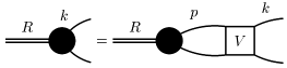
Figure 1: Diagrammatic representation of the Bethe-Salpeter equation. The blob represents the vertex function $\Gamma$.

Looking at Eq. (2), in order to project the wave function exactly, we must know the analytic structure of the bound-state vertex function. If the vertex function $\Gamma(k,R)$ had no poles in $\operatorname{k^{--}}$, then our task would be simple: the light-front projection of $\Psi_{BS}$ would pick up contributions only from the poles of the propagator $G(k,R)$. Next we observe from Eq. (1), that the $\operatorname{k^{--}}$ dependence of the interaction $V(k,p)$ must give rise to the $\operatorname{k^{--}}$ poles of the vertex function $\Gamma(k,R)$. Hence an instantaneous interaction gives rise to an instantaneous vertex and a simple light-front projection (see e.g. Einhorn:1976uz ).

On the other hand, constituent quark models often assume a less restrictive simplification of the analytic structure of the vertex (see e.g. Jaus:zv ) in order to permit the light-cone projection. We shall show that this assumption along with the presumed covariance of the quark model often implies instantaneous vertices. For any momentum $p$, let us denote the on-shell energy $p^{-}_{\text{on}}=m^{2}/2p^{+}$. The propagator $G(k,R)$ has two poles

$$\begin{cases}k^{-}_{a}=k^{-}_{\text{on}}-\frac{\operatorname{i\epsilon}}{x}\\ k^{-}_{b}=R^{-}+(k-R)^{-}_{\text{on}}-\frac{\operatorname{i\epsilon}}{x-1}.\end{cases}$$ (5)

Notice that although we work in $(1+1)$ dimensions, the results are trivial to extend to $(3+1)$ dimensions because the imaginary parts of poles have precisely the same dependence on (only) the plus-momenta. This remark applies not only to this section but to the rest of this work.

In constituent quark models $\Gamma$ is assumed to have no poles in the upper-half $k^{-}$-plane for $0<x<1$. Since the light-front wave function is proportional to $\theta[x(1-x)]$, in light of Eq. (5) we further require any poles of $\Gamma$ to lie in the upper-half plane for $x<0$ and in the lower-half plane for $x>1$. With these restrictions Eq. (4) dictates the form of the constituent quark wave function

$$\psi(x)=\operatorname{D_{\text{W}}}(x|M^{2})\Gamma(k_{b},R)\theta[x(1-x)],$$ (6)

where we have defined the Weinberg propagator as

$$\operatorname{D_{\text{W}}}(x|M^{2})=\frac{1}{M^{2}-\frac{m^{2}}{x(1-x)}}$$ (7)

and used the abbreviation $\Gamma(k_{b},R)$ to denote evaluation at the pole $k^{-}=k^{-}_{b}$ appearing in Eq. (5).

When we calculate the (elastic) electromagnetic form factor for these constituent quark models (see Figure 2), we are confronted with more poles.

Figure 2: Covariant diagram for the electromagnetic form factor. Labels $a,b$ and $c$ denote subscripts used for on-shell energy poles.

Let $\Delta^{+}=-\zeta P^{+}<0$ be the plus-component of the momentum transfer between initial and final state mesons. The form factor is then

$$F(t)\propto\int\frac{(2x-\zeta)\Gamma(k,P)\Gamma^{*}(k+\Delta,P+\Delta)\;d^{2}k}{[k^{2}-m^{2}][(P-k)^{2}-m^{2}][(k+\Delta)^{2}-m^{2}]}$$ (8)

The $k^{-}$-poles from the propagators are $k^{-}_{a},k^{-}_{b}$ defined in (5) and $k^{-}_{c}=-\Delta^{-}+(k+\Delta)^{-}_{\text{on}}-\frac{\operatorname{i\epsilon}}{x-\zeta}$.

Given this pole structure, the contributions to $F(t)$ are proportional to $\theta[x(1-x)]$. In the region $x<\zeta$, closing the contour in the upper-(lower-) half plane will enclose possible poles of the final (initial) vertex. As one can see from considering the region $x>\zeta$, the form factor can be determined solely from $\operatorname{Res}(k^{-}_{b})$. In $(3+1)$ dimensions, where we are free to choose frames in which $\zeta=0$, this is the only contribution to the form factor. But if $\zeta\neq 0$, the additional poles from vertices in the region $x<\zeta$ are required by Lorentz invariance.

The authors Ji:2000fy advocate no modification to the pole structure of Eq. (8) due to the vertices. Closing the contour in the lower-half plane, they pick up the residue at $k^{-}_{a}$ without any contributions from poles of the initial-state vertex. Such poles cannot lie in the upper-half plane for $x<\zeta$ since the form of $\psi$ would be both frame dependent and contrary to that of Eq. (6) (the $(3+1)$-dimensional version of which is employed by Ji:2000fy ). Thus the authors are actually assuming there are no poles of the Bethe-Salpeter vertex Tiburzi:2001je .

Returning to the definition of the wave function (4) under the premise of a vertex devoid of poles, we now find $\Gamma(k_{b},P)=\Gamma(k_{a},P)$, which we shall call pole symmetry. This symmetry is essential for making contact with the Drell-Yan formula Drell:1970km , since for $x>\zeta$ both initial- and final- state vertices may be expressed in terms of wave functions. When $x<\zeta$, however, the final-state vertex becomes $\Gamma^{*}(k_{a}+\Delta,P+\Delta)$ which cannot be expressed in terms of $\psi^{*}(x^{\prime})$ (where $x^{\prime}=\frac{x-\zeta}{1-\zeta}$) even with pole symmetry. Such a vertex is referred to as a non-wave function vertex. Understanding and dealing with such objects from the perspective of time-ordered perturbation theory is the primary goal of this paper.

Because these constituent quark models are presumed covariant, Eq. (8) converges. This enables us to relate an initial-state non-wave function vertex to the final-state non-wave function vertex encountered above via integrating around a circle at infinity. Equating the sum of residues $\operatorname{Res}(k^{-}_{a})+\operatorname{Res}(k^{-}_{b})+\operatorname{Res}(k^{-}_{c})=0$, we find

$$\frac{\Gamma^{*}(k_{a}+\Delta,P^{\prime})}{\Gamma^{*}(k_{b}+\Delta,P^{\prime})}(k^{-}_{b}-k^{-}_{c})-\frac{\Gamma(k_{c},P)}{\Gamma(k_{b},P)}(k^{-}_{b}-k^{-}_{a})=k^{-}_{a}-k^{-}_{c}.$$ (9)

This relation holds for the class of models for which the pole structure of Eq. (8) is not modified by the vertices. The ratio structure of the vertices does not allow for a common factor $k^{-}_{a}-k^{-}_{c}$ in the two terms in Eq. (9). The equality then depends on delicate cancellations between initial- and final- state vertices, which in general are unrelated. The philosophy of constituent quark model phenomenology is to choose the form of $\psi$ and hence the form of $\Gamma$. Treating $\Gamma$ free, equality can only hold if both ratios are one. This yields the restriction

$$\frac{\partial}{\partial\Delta^{-}}\Gamma(k_{c},P)=0.$$ (10)

But $\Delta^{-}$ only enters $\Gamma(k_{c},P)$ through $k^{-}=k^{-}_{c}$. Hence $\Gamma$ is independent of $k^{-}$. In general, of course, the vertex $\Gamma$ not only has light-front energy dependence but poles as well. As we shall see below, the light-front reduction of the Bethe-Salpeter equation is a procedure for approximating the poles of the vertex function. Moreover when applied to current matrix elements, these poles generate higher Fock state contributions.

III Light-front reduction

In this section, we review the reduction scheme set up in Sales:1999ec since their notation, while useful, is unfamiliar. Additionally we resolve a peccadillo intrinsically related to non-wave function vertices. Next we give an intuitive picture for the reduction and finally construct the gauge invariant current for the calculation of form factors on the light-front.

Above we have removed overall momentum-conserving delta functions, e.g. our propagator $G(k,R)$ is the momentum space version of $G(R)$ defined by $\langle R^{\prime}|G|R\rangle=(2\pi)^{2}\delta^{(2)}(R^{\prime}-R)G(R)$. In terms of these fully two-dimensional quantities, the Lippmann-Schwinger equation for the two-particle transition matrix $T$ appears as

$$T=V+VGT.$$ (11)

A pole in the $T$-matrix (at some $R^{2}=M^{2}$, say) corresponds to a two-particle bound state. Investigation of the pole’s residue gives the Bethe-Salpeter equation for the bound-state vertex $\Gamma$

$$\Gamma=VG\Gamma.$$ (12)

The Bethe-Salpeter amplitude $\Psi$ is defined to be $G\Gamma$. Following Sales:1999ec , we denote quantities able to be rendered in position or momentum space with bras and kets. We will employ this notation only for quantities that have been stripped of their overall momentum-conserving delta functions, for example $\Gamma(k,R)=\langle k|\Gamma_{R}\rangle$, where $R$ is used as a label for the bound state for which $R^{2}=M^{2}$.

III.1 The scheme

To reduce the Lippmann-Schwinger equation to a light-front version, we must introduce an auxiliary Green’s function $\operatorname{\tilde{G}}$ in place of $G$ (as in Woloshyn:wm ). Thus we have

$$T=W+W\operatorname{\tilde{G}}T,$$ (13)

provided that

$$W=V+V(G-\operatorname{\tilde{G}})W.$$ (14)

Taking residues of Eq. (13) gives us an alternate way to express the bound state vertex function

$$\Gamma=W\operatorname{\tilde{G}}\Gamma.$$ (15)

To choose a light front reduction, $\operatorname{\tilde{G}}$ must inherently be related to projection onto the initial surface $x^{+}=0$. For simplicity, we denote the integration $\int\frac{d\operatorname{k^{--}}}{2\pi}\langle\operatorname{k^{--}}|\mathcal{O}(R)=\Big{|}\mathcal{O}(R)$. With this notation, we will always work in $(1+1)$-dimensional momentum space for which the only sensible matrix elements of $\Big{|}\mathcal{O}(R)$ are of the form $\langle\operatorname{k^{+}}|\;\Big{|}\mathcal{O}(R)|\operatorname{p^{--}},\operatorname{p^{+}}\rangle$. The operator $\mathcal{O}(R)\Big{|}$ is defined similarly. For a useful reduction scheme (one that preserves unitarity), we must have $\Big{|}G(R)\Big{|}=\Big{|}\operatorname{\tilde{G}}(R)\Big{|}$. The simplest choice of $\operatorname{\tilde{G}}$ that results in time-ordered perturbation theory requires

$$\operatorname{\tilde{G}}(R)=G(R)\Big{|}g^{-1}(R)\;\Big{|}G(R),$$ (16)

where the reduced disconnected propagator $g(R)$ is defined by the matrix elements

$$\langle xR^{+}|\;\Big{|}G(R)\Big{|}\;|yR^{+}\rangle=\langle xR^{+}|g(R)|yR^{+}\rangle,$$ (17)

explicitly this forces

$$\langle xR^{+}|g(R)|yR^{+}\rangle=2\pi\delta(xR^{+}-yR^{+})\\ \times\theta[x(1-x)]\frac{2\pi i}{2R^{+}x(1-x)}\operatorname{D_{\text{W}}}(x|R^{2}).$$ (18)

The inverse propagator $g^{-1}(R)$ can then be constructed, bearing in mind $g^{-1}(R)$ only exits in the subspace where $g(R)$ is non-zero. Explicitly

$$\langle xR^{+}|g^{-1}(R)|yR^{+}\rangle=2\pi\delta(xR^{+}-yR^{+})\\ \times\theta[x(1-x)]\frac{2R^{+}x(1-x)}{2\pi i}\operatorname{D_{\text{W}}}^{-1}(x|R^{2}).$$ (19)

This forces

$$\langle xR^{+}|g^{-1}(R)g(R)|yR^{+}\rangle=2\pi\delta(xR^{+}-yR^{+})\theta[x(1-x)],$$ (20)

which is unity restricted to the subspace where the operators $g(R)$ and $g^{-1}(R)$ are defined. We are more careful about this point than the authors Sales:1999ec since the consequences of Eq. (19) are essential for dealing with instantaneous interactions. Notice $\operatorname{\tilde{G}}(R)$ defined in Eq. (16) is non-zero only for plus-momentum fractions between zero and one.

The reduced transition matrix $t(R)$ is

$$t(R)=g^{-1}(R)\Big{|}\operatorname{\tilde{G}}(R)T(R)\operatorname{\tilde{G}}(R)\Big{|}g^{-1}(R)$$ (21)

Taking the residue of Eq. (21) at $R^{2}=M^{2}$, gives a homogeneous equation for the reduced vertex function $\gamma$

$$|\gamma_{R}\rangle=w(R)g(R)|\gamma_{R}\rangle,$$ (22)

where the reduced auxiliary kernel is

$$w(R)=g^{-1}(R)\Big{|}G(R)W(R)G(R)\Big{|}g^{-1}(R).$$ (23)

Given this structure, the reduced kernel $w(x,y|R^{2})\equiv\langle xR^{+}|w(R)|yR^{+}\rangle$ will always be $\propto\theta[x(1-x)]\theta[y(1-y)]$. Moreover the reduced vertex $\gamma(x|M^{2})\equiv\langle xR^{+}|\gamma_{R}\rangle\propto\theta[x(1-x)]$ as a result of Eq. (22).

From (22) we can define the light-front wave function $|\psi_{R}\rangle\equiv g(R)|\gamma_{R}\rangle$, notice this too restricts the momentum fraction $x$: $\psi(x)\propto\theta[x(1-x)]$. By iterating the Lippmann-Schwinger equation for $T$ twice, it is possible to relate $T$ to $t$ and thereby construct $T$ given $t$, which is clearly not possible from the definition (21). Taking the residue of this relation between $T$ and $t$ yields the reduced-to-covariant conversion between bound-state vertex functions, namely

$$|\Gamma_{R}\rangle=W(R)G(R)\Big{|}\;|\gamma_{R}\rangle.$$ (24)

Finally, we can manipulate the covariant Bethe-Salpeter amplitude into the form

$$|\Psi_{R}\rangle=\Bigg{(}1+\Big{(}G(R)-\operatorname{\tilde{G}}(R)\Big{)}W(R)\Bigg{)}G(R)\Big{|}\;|\gamma_{R}\rangle,$$ (25)

which justifies the interpretation of $|\psi_{R}\rangle$ as the light-front wave function since $\Big{|}\;|\Psi_{R}\rangle=|\psi_{R}\rangle$.

While all light-front reduction schemes when summed to all orders yield the $x^{+}=0$ projection of the Bethe-Salpeter equation, the choice of $\operatorname{\tilde{G}}(R)$ in Eq. (16) generates a kernel calculated in light-front time-ordered perturbation theory. Lastly the normalization of the covariant and reduced wave function is discussed in future .

III.2 An interpretation for the reduction

The heart of our intuition about the light cone lies in integrating out the minus-momentum dependence of the covariant wave function. So we merely cast the formal reduction in a way which highlights the contributions from poles of the vertex function.

Utilizing Eqs. (15) and (24), we can show

$$\operatorname{\tilde{G}}(R)|\Gamma_{R}\rangle=G(R)\Big{|}\;|\gamma_{R}\rangle.$$ (26)

Thus the appearance of $\operatorname{\tilde{G}}(R)|\Gamma_{R}\rangle$ has the form of an instantaneous approximation since Eq. (26) shows that it has no minus-momentum poles besides those of the propagator $G(R)$.

This instantaneous approximation appears in determining the light-front wave function. Using Eqs. (14) and (25), we have

$$|\psi_{R}\rangle=\Big{|}G(R)V(R)\\ \times\sum_{j=0}^{\infty}\Big{[}\Big{(}G(R)-\operatorname{\tilde{G}}(R)\Big{)}V(R)\Big{]}^{j}G(R)\Big{|}\;|\gamma_{R}\rangle.$$ (27)

From truncating the series in $G(R)-\operatorname{\tilde{G}}(R)$ at some $j=n-1$ and using a consistent approximation to Eq. (24), we are led to the approximate solution

$$|\psi^{(n)}\rangle=\Big{|}(GV)^{n}\operatorname{\tilde{G}}|\Gamma\rangle,$$ (28)

after having used Eq. (26). Thus at any order $n$ in the formal reduction scheme, we have iterated the covariant Bethe-Salpeter equation $n$-times and subsequently made an instantaneous approximation via Eq. (26). Retaining the minus-momentum dependence in $V$ to $n^{\text{th}}$ order allows for an $n^{\text{th}}$-order approximation to the vertex function’s poles.

III.3 Current in the reduced formalism

Here we extend the formalism presented so far to include current matrix elements between bound states. We do so in a gauge invariant fashion following Gross:bu . Our notation, however, is more in line with the elegant method of gauging equations presented in Kvinikhidze:1998xn . This latter general method extends to bound systems of more than two particles.

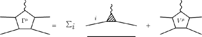
Figure 3: Graphical depiction of the irreducible five-point function $\Gamma^{\mu}$ as sum of impulse terms and a gauged interaction. By construction, $\Gamma^{\mu}$ is gauge invariant.

Consider first the full four-point function $G^{(4)}$ defined by

$$G^{(4)}=G+GTG.$$ (29)

For later use, it is important to note that the residue of $G^{(4)}(R)$ at the bound state pole $R^{2}=M^{2}$ is $-i|\Psi_{R}\rangle\langle\Psi_{R}|$. Using the Lippmann-Schwinger equation for $T$, we can show the four-point function satisfies

$$G^{(4)}=G+GVG^{(4)}.$$ (30)

To discuss electromagnetic current matrix elements, we will need the three-point function $d_{i}^{\mu}$ where the label $i$ denotes particle number. We define an irreducible three-point function $\Gamma_{i}^{\mu}$ in the obvious way

$$d_{i}^{\mu}=d_{i}\Gamma_{i}^{\mu}d_{i}.$$ (31)

Now we need to relate the one-particle electromagnetic vertex function to the $T$ matrix. Let $j^{\mu}$ denote the electromagnetic coupling to the constituent particles (since our particles are scalars $j^{\mu}=\overset{\leftrightarrow}{\partial}{}^{\mu}$). Since the electromagnetic three-point function $\Gamma_{i}^{\mu}$ is irreducible, we have

$$\Gamma_{i}^{\mu}=G^{-1}G^{(4)}j^{\mu}$$ (32)

and by using the definition of $G^{(4)}$ Eq. 29, we have the desired relation

$$\Gamma_{i}^{\mu}=j^{\mu}+TGj^{\mu}$$ (33)

Notice the right hand side lacks the particle label $i$. In the first term, the bare coupling acts on the $i$th particle while in the second term the bare coupling does not act on the $i$th particle. For this reason we have dropped the label which will always be clear from context.

In considering two propagating particles’ interaction with a photon, the above definitions lead us to the impulse approximation to the current

$$\Gamma_{0}^{\mu}=\Gamma_{1}^{\mu}d_{2}^{-1}+d_{1}^{-1}\Gamma_{2}^{\mu}.$$ (34)

Additionally the photon could couple to interacting particles. Define a gauged interaction $V^{\mu}$ topologically by attaching a photon to the kernel in all possible places. This leads us to the irreducible electromagnetic vertex $\Gamma^{\mu}$ defined as (see Figure 3)

$$\Gamma^{\mu}=\Gamma_{0}^{\mu}+V^{\mu},$$ (35)

which is gauge invariant by construction.

Lastly to calculate matrix elements of the current between bound states it is useful to define a reducible five-point function (see Figure 4)

$$G^{(5)\;\mu}=G^{(4)}\Gamma^{\mu}G^{(4)}.$$ (36)

Having laid out the necessary facts about electromagnetic vertex functions and gauge invariant currents, we can now specialize to their matrix elements between bound states by taking appropriate residues of Eq. (36). The form factor is then

$$-i(P^{\prime\mu}+P^{\mu})F(t)=\langle\Psi_{P^{\prime}}|\Gamma^{\mu}(-\Delta)|\Psi_{P}\rangle,$$ (37)

where $P^{\prime\mu}=P^{\mu}+\Delta^{\mu}$ and $t=\Delta^{2}$.

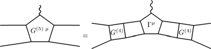
Figure 4: Graphical depiction of the five-point function $G^{(5)\;\mu}$. The irreducible five-point function is the gauge invariant $\Gamma^{\mu}$.

IV Two models

IV.1 Wave functions

To say anything less than general, we must know the minus-momentum dependence of the interaction. We therefore adopt a weakly coupled, one-boson exchange model for $V$ (the so-called ladder approximation). Supposing the boson mass is $\mu$ and the coupling constant $g$, we have

$$V(k,p)=\frac{-g^{2}}{(p-k)^{2}-\mu^{2}+\operatorname{i\epsilon}}$$ (38)

where the energy pole (with respect to $p$) of the interaction is

$$p^{-}_{v}=\operatorname{k^{--}}+\frac{\mu^{2}}{2(\operatorname{p^{+}}-\operatorname{k^{+}})}-\frac{\operatorname{i\epsilon}}{2(\operatorname{p^{+}}-\operatorname{k^{+}})}.$$ (39)

This interaction is non-local in space-time and hence does not have an instantaneous piece. The reduced kernel Eq. (23) is consequently made up of retarded terms (i.e. dependent on the eigenvalue $M^{2}$) where higher order in $G-\operatorname{\tilde{G}}$ means more particles propagating at a given instant of light-cone time (see, e.g. Sales:1999ec ). The leading-order equation for $\psi$ from Eq. (22) is the Weinberg equation Weinberg:1966jm

$$\psi(x)=-\operatorname{D_{\text{W}}}(x|M^{2})\int_{0}^{1}\frac{w(x,y|M^{2})\psi(y)}{2(2\pi)y(1-y)}dy.$$ (40)

with the time-ordered one-boson exchange potential (see Figure 5) calculated to leading order from Eq. (23)

$$w(x,y|M^{2})=\frac{-g^{2}}{x-y}\theta[x(1-x)]\theta[y(1-y)]\\ \times\Big{[}\theta(x-y)D(x,y|M^{2})-\{x\leftrightarrow y\}\Big{]},$$ (41)

where

$$D^{-1}(x,y|M^{2})=M^{2}-\frac{m^{2}}{y}-\frac{\mu^{2}}{x-y}-\frac{m^{2}}{1-x}.$$ (42)

We can obtain Eq. (40) most simply by iterating the Bethe-Salpeter equation once (see section III.2) and then projecting onto the light cone.

Figure 5: Diagrammatic representation of the one-boson exchange potential $w(x,y|M^{2})$ appearing in Eq. (41).

In the limit $\mu^{2}\gg m^{2},M^{2}$, the interaction becomes approximately instantaneous, which suggests we separate out an instantaneous piece $V_{o}$:

$$V(k,p)=V_{o}+[V(k,p)-V_{o}],$$ (43)

where

$$V_{o}=V_{o}(x,y)=\frac{-g^{2}\theta(x-y)}{E^{2}(x-y)-\mu^{2}}+\frac{-g^{2}\theta(y-x)}{E^{2}(y-x)-\mu^{2}},$$ (44)

with $E$ as a parameter to be chosen. Of course other choices of $V_{o}$ are possible. We choose the above form of $V_{o}$ for two reasons. First is the form of the instantaneous approximation wave function $\phi(x)$. When we write the potential as Eq. (43), we expand Eq. (14) to first order in $g^{2}$ as

$$W=V_{o}+(V-V_{o})+(V-V_{o})\Big{(}G-\operatorname{\tilde{G}}\Big{)}(V-V_{o}).$$ (45)

To zeroth order in $G-\operatorname{\tilde{G}}$ and $V-V_{o}$, the equation for $\phi$ is

$$\phi(x)=-\operatorname{D_{\text{W}}}(x|M^{2})\int_{0}^{1}\frac{w_{o}(x,y)\phi(y)}{2(2\pi)y(1-y)}dy,$$ (46)

where by Eq. (23), the reduced instantaneous potential is merely $w_{o}(x,y)=\theta[x(1-x)]\theta[y(1-y)]V_{o}(x,y)$. In the instantaneous limit, $\mu^{2}\gg m^{2},M^{2}$ solutions to Eqs. (40) and (46) coincide—both wave functions approach $\sim\operatorname{D_{\text{W}}}(x,4m^{2})$. Secondly, we preserve the contact interaction limit by excluding from $V_{o}$ the factor $\theta[x(1-x)]\theta[y(1-y)]$. That is, when $\{\mu^{2},g^{2}\}\to\infty$ with $g^{2}/\mu^{2}$ fixed (or equivalently $E\to 0$) we have the contact interaction $V_{o}\to g^{2}/\mu^{2}$, which rightly knows nothing about the momentum fractions $x$ and $y$.

We shall now investigate contributions to the form factors for each of the models Eqs. (38) and (44).

IV.2 Form factors

From Eq. (37) we can calculate the form factors for each of the models (38) and (44) in the reduced formalism. Working in perturbation theory, we separate out contributions up to first order by using Eq. (25) to first order in $G-\operatorname{\tilde{G}}$ and $\Gamma^{\mu}$ (35) in the first Born approximation. The matrix element $J^{\mu}=\langle\Psi_{P^{\prime}}|\Gamma^{\mu}(-\Delta)|\Psi_{P}\rangle$ then appears for a model with some kernel $V$

$$J^{\mu}\approx\;\langle\gamma_{P^{\prime}}|\;\Big{|}G(P^{\prime})\Big{(}1+V(P^{\prime})(G(P^{\prime})-\operatorname{\tilde{G}}(P^{\prime}))\Big{)}\\ \times\Big{(}\overset{\leftrightarrow}{\partial}{}^{\mu}(-\Delta)d_{2}^{-1}+V(-\Delta)G(-\Delta)\overset{\leftrightarrow}{\partial}{}^{\mu}(-\Delta)d_{2}^{-1}\Big{)}\\ \times\Big{(}1+(G(P)-\operatorname{\tilde{G}}(P))V(P)\Big{)}G(P)\Big{|}\;|\gamma_{P}\rangle\\ =\Big{(}J^{\mu}_{\text{LO}}+\delta J^{\mu}_{i}+\delta J^{\mu}_{f}+\delta J^{\mu}_{\gamma}\Big{)}+\mathcal{O}[V^{2}],$$ (47)

with the leading-order result

$$J^{\mu}_{\text{LO}}=\langle\gamma_{P^{\prime}}|\;\Big{|}G(P^{\prime})\overset{\leftrightarrow}{\partial}{}^{\mu}(-\Delta)d_{2}^{-1}G(P)\Big{|}\;|\gamma_{P}\rangle.$$ (48)

The first-order terms are

$$\delta J^{\mu}_{i}=\langle\gamma_{P^{\prime}}|\;\Big{|}G(P^{\prime})\overset{\leftrightarrow}{\partial}{}^{\mu}(-\Delta)d_{2}^{-1}\\ \times\Big{(}G(P)-\operatorname{\tilde{G}}(P)\Big{)}V(P)G(P)\Big{|}\;|\gamma_{P}\rangle$$ (49)

$$\delta J^{\mu}_{f}=\langle\gamma_{P^{\prime}}|\;\Big{|}G(P^{\prime})V(P^{\prime})\Big{(}G(P^{\prime})-\operatorname{\tilde{G}}(P^{\prime})\Big{)}\\ \times\overset{\leftrightarrow}{\partial}{}^{\mu}(-\Delta)d_{2}^{-1}G(P)\Big{|}\;|\gamma_{P}\rangle$$ (50)

$$\delta J^{\mu}_{\gamma}=\langle\gamma_{P^{\prime}}|\;\Big{|}G(P^{\prime})\Big{(}V(-\Delta)G(-\Delta)\overset{\leftrightarrow}{\partial}{}^{\mu}(-\Delta)\Big{)}\\ \times d_{2}^{-1}G(P)\Big{|}\;|\gamma_{P}\rangle.$$ (51)

The labels indicate the intuition behind the reduction scheme (seen in section III.2): the term $\delta J^{\mu}_{f}$ arises from one iteration of the covariant Bethe-Salpeter equation for the final-state vertex followed by an instantaneous approximation (26), $\delta J^{\mu}_{i}$ arises in the same way from the initial state and $\delta J^{\mu}_{\gamma}$ comes from one iteration of the Lippmann-Schwinger equation (11).

Because the leading-order expression (48) is independent of the kernel $V$, the result will have the same form for both models. Using the effective resolution of unity, the above expression converts into

$$J^{\mu}_{\text{LO}}=\int\frac{d^{2}p}{(2\pi)^{2}}\;\frac{d^{2}k}{(2\pi)^{2}}\langle\gamma_{P^{\prime}}|\operatorname{p^{+}}\rangle\\ \times\langle p|G(P^{\prime})\overset{\leftrightarrow}{\partial}{}^{+}(-\Delta)d_{2}^{-1}G(P)|k\rangle\;\langle\operatorname{k^{+}}|\gamma_{P}\rangle.$$ (52)

Bearing in mind the delta function present in $G(R)$, we have the factor

$$\langle p|\overset{\leftrightarrow}{\partial}{}^{+}(-\Delta)|k\rangle=-i(2\operatorname{k^{+}}+\Delta^{+})(2\pi)^{2}\delta^{2}(p-k-\Delta).$$ (53)

Now define $x=\operatorname{k^{+}}/P^{+}$ and $\Delta^{+}=-\zeta P^{+}$ as above and denote the reduced vertex $\langle\operatorname{k^{+}}|\gamma_{R}\rangle=\gamma(x|M^{2})$. The leading-order contribution is then

$$J^{+}_{\text{LO}}=\int\frac{d^{2}k}{(2\pi)^{2}}\gamma^{*}(x^{\prime}|M^{2})d(k+\Delta)\\ \times\big{(}2x-\zeta\big{)}d(k)d(P-k)\gamma(x|M^{2}),$$ (54)

where $x^{\prime}=\frac{x-\zeta}{1-\zeta}$. Eq. (54) is quite similar to (8). For $x>\zeta$ evaluation is straightforward and leads to

$$F_{LO}(t)=\frac{\theta(x-\zeta)}{1-\zeta/2}\int\frac{dx}{2(2\pi)}\frac{2x-\zeta}{x(1-x)x^{\prime}}\psi^{*}(x^{\prime})\psi(x),$$ (55)

for the non-instantaneous case. For the instantaneous case $F_{LO}(t)$, replace $\psi$ with $\phi$.

On the other hand, we know from section II the region $x<\zeta$ contains a non-wave function vertex (see Figure 6).

Figure 6: The $Z$-graph confronting evaluation of the electromagnetic form factor

However, evaluation of Eq. (54) with reduced vertices is subtly different than in section II. Quite simply, the term $\gamma^{*}(x^{\prime}|M^{2})=0$ by virtue of Eq. (22) because $x^{\prime}<0$. Thus there is no contribution at leading order for $x<\zeta$.

The first-order terms depend explicitly on the interaction and will hence be considerably different for each of the models. We consider each model separately.

IV.2.1 Non-instantaneous case

Evaluating contributions at first order for the non-instantaneous interaction Eq. (38) is complicated by the presence of poles in the interaction (cf Eq. (39)). First we evaluate the first Born term $\delta J^{\mu}_{\gamma}$ in Eq. (51). After careful evaluation of the two minus-momentum integrals, we have the contribution to $\delta J^{+}_{\gamma}$ for $x>\zeta$

$$\delta J^{+}_{A}=\int\frac{\theta(x-\zeta)\;dxdy\;(2x-\zeta)}{16\pi^{2}xx^{\prime}y(1-y)y^{\prime}}\psi^{*}(y^{\prime})\\ \times D(y^{\prime},x^{\prime}|M^{2})\frac{g^{2}\theta(y-x)}{y-x}D(y,x|M^{2})\psi(y),$$ (56)

where $y^{\prime}=\frac{y-\zeta}{1-\zeta}$. This contribution corresponds to diagram $A$ in Figure 7.

Figure 7: Diagrams which contribute to the form factor to first order in $G-\operatorname{\tilde{G}}$ for the non-instantaneous case (for $x>\zeta$).

Additionally using $x^{\prime\prime}=x/\zeta$, we have for $x<\zeta$

$$\delta J^{+}_{D}=\int\frac{\theta(\zeta-x)\;dxdy\;(2x-\zeta)/\zeta}{16\pi^{2}y(1-y)y^{\prime}x^{\prime\prime}(1-x^{\prime\prime})}\psi^{*}(y^{\prime})\\ \times\operatorname{D_{\text{W}}}(x^{\prime\prime}|t)\frac{g^{2}\theta(y-x)}{y-x}D(y,x|M^{2})\psi(y),$$ (57)

which corresponds to diagram $D$ in Figure 8.

Figure 8: The remaining diagrams (characterized by $x<\zeta$) for the electromagnetic form factor at first order in $G-\operatorname{\tilde{G}}$ for the non-instantaneous case.

The initial-state iteration term $\delta J^{\mu}_{i}$ in Eq. (51) is complicated by the subtraction of the two-particle reducible contribution

$$-\langle\gamma_{P^{\prime}}|\;\Big{|}G(P^{\prime})\overset{\leftrightarrow}{\partial}{}^{\mu}(-\Delta)d_{2}^{-1}\operatorname{\tilde{G}}(P)V(P)G(P)\Big{|}\;|\gamma_{P}\rangle\\ =-\langle\gamma_{P^{\prime}}|\;\Big{|}G(P^{\prime})\overset{\leftrightarrow}{\partial}{}^{\mu}(-\Delta)d_{2}^{-1}G(P)\Big{|}\;|\gamma_{P}\rangle.$$ (58)

Thus this term merely removes contributions which can be reduced into the initial-state wave function. Evaluation of the two minus-momentum integrals yields a contribution for $x>\zeta$ to $\delta J^{+}_{i}$

$$\delta J^{+}_{B}=\int\frac{\theta(x-\zeta)\;dxdy\;(2x-\zeta)}{16\pi^{2}xx^{\prime}(1-x^{\prime})y(1-y)}\psi^{*}(x^{\prime})\\ \times D(y^{\prime},x^{\prime}|M^{2})\frac{g^{2}\theta(y-x)}{y-x}D(y,x|M^{2})\psi(y),$$ (59)

which corresponds to diagram $B$ in Figure 7. On the other hand, for $x<\zeta$, we have the non-wave function vertex $\gamma^{*}(x^{\prime}|M^{2})$ for the final state, which vanishes. Similarly the $\operatorname{\tilde{G}}(P)$ term vanishes. Thus there is no contribution to $\delta J^{\mu}_{i}$ for $x<\zeta$.

Finally there is the final-state iteration term $\delta J^{\mu}_{f}$ in Eq. (51). There are only two types of contributions. For $x>\zeta$, that which can be reduced in to the final-state wave function is subtracted by $\operatorname{\tilde{G}}$. The remaining term is:

$$\delta J^{+}_{C}=\int\frac{\theta(x-\zeta)\;dxdy^{\prime}(2x-\zeta)}{16\pi^{2}x(1-x)x^{\prime}y^{\prime}(1-y^{\prime})}\psi^{*}(y^{\prime})\\ \times D(y^{\prime},x^{\prime}|M^{2})\frac{g^{2}\theta(y-x)}{y-x}D(y,x|M^{2})\psi(x),$$ (60)

where $y=\zeta+(1-\zeta)y^{\prime}$. This corresponds to diagram $C$ in Figure 7. For $x<\zeta$, the subtraction term vanishes since $x^{\prime}<0$ for which $\operatorname{\tilde{G}}(P^{\prime})=0$. The remaining term in $\delta J^{+}_{f}$ gives a contribution

$$\delta J^{+}_{E}=\int\frac{\theta(\zeta-x)\;dxdy^{\prime}(2x-\zeta)/\zeta}{16\pi^{2}(1-x)x^{\prime\prime}(1-x^{\prime\prime})y^{\prime}(1-y^{\prime})}\psi^{*}(y^{\prime})\\ \times\operatorname{D_{\text{W}}}(x^{\prime\prime}|t)\frac{g^{2}\theta(y-x)}{y-x}D(y,x|M^{2})\psi(x),$$ (61)

which corresponds to diagram $E$ in Figure 8. To summarize, the non-valence correction to the form factor in the non-instantaneous case is

$$\delta F_{NI}=\frac{1}{1-\zeta/2}\Big{[}\delta J^{+}_{A}+\delta J^{+}_{B}+\delta J^{+}_{C}+\delta J^{+}_{D}+\delta J^{+}_{E}\Big{]},$$ (62)

and there are no non-wave function terms.

IV.2.2 Instantaneous case

The case of an instantaneous interaction is quite different due to the absence of light-front energy poles in $V_{o}$. Note we are working with Eq. (45) to zeroth order in $G-\operatorname{\tilde{G}}$ and $V-V_{o}$. The first term in Eq. (51) we consider, is the Born term $\delta J^{\mu}_{\gamma}$. The pole structure leads only to a contribution for $x<\zeta$:

$$\delta J^{+}_{1}=-\int\frac{\theta(\zeta-x)\theta(y-x)\;dxdy\;(2x-\zeta)/\zeta}{16\pi^{2}y(1-y)y^{\prime}x^{\prime\prime}(1-x^{\prime\prime})}\\ \times\phi^{*}(y^{\prime})\operatorname{D_{\text{W}}}(x^{\prime\prime}|t)V_{o}(x^{\prime\prime},y^{\prime\prime})\phi(y),$$ (63)

and is depicted by the first diagram in Figure 9. The interaction along the way to the photon vertex is crossed and represents pair production off the quark line ($x^{\prime\prime}>1$).

Figure 9: Diagrams with crossed interactions necessary to calculate the form factor in the region $x<\zeta$ for the instantaneous case.

The next term $\delta J^{\mu}_{i}$ simplifies considerably due to the absence of light-cone time dependence in $V_{o}$. As above, the final state vertex restricts $\zeta<x<1$. But then we are confronted with a factor $\langle k|\Big{(}G(P)-\operatorname{\tilde{G}}(P)\Big{)}\Big{|}=0$ since $x>0$. Thus $\delta J^{\mu}_{i}=0$.

The last term we must consider is $\delta J^{\mu}_{f}$, in which we have the factor $\Big{|}\Big{(}G(P^{\prime})-\operatorname{\tilde{G}}(P^{\prime})\Big{)}|k+\Delta\rangle$. This is zero for $x-\zeta>0$, else $\operatorname{\tilde{G}}(P^{\prime})=0$ by virtue of Eq. (16) and Eq. (19). Thus we only have a contribution for $x<\zeta$ which is from $\Big{|}G(P^{\prime})|k+\Delta\rangle$. The expression for this contribution is

$$\delta J^{+}_{2}=-\int\frac{\theta(\zeta-x)\theta(y-x)dxd\operatorname{y^{\prime}}(2x-\zeta)/\zeta}{16\pi^{2}(1-x)\operatorname{x^{\prime\prime}}(1-\operatorname{x^{\prime\prime}})\operatorname{y^{\prime}}(1-\operatorname{y^{\prime}})}\\ \times\phi^{*}(\operatorname{y^{\prime}})w_{o}(y^{\prime},x^{\prime})\operatorname{D_{\text{W}}}(\operatorname{x^{\prime\prime}}|t)\phi(x),$$ (64)

and is depicted on the right in Figure 9. The interaction again is crossed ($x^{\prime}<0$) and represents pair production. With Eqs. (63) and (64), we have both bare-coupling pieces of the full Born series for the photon vertex (further terms in the series, which result from higher order terms in the expansion of $W$, add interaction blocks to each diagram on the quark-antiquark pair’s path to annihilation). In this way we recover the Green’s function from summing the Born series Einhorn:1976uz ; Tiburzi:2001je . Notice also the above form of $\delta J^{+}_{2}$ is what one would obtain from extending the definition of $\gamma$ as a non-wave function vertex Einhorn:1976uz . For the case of an instantaneous interaction, the light-front Bethe-Salpeter formalism automatically incorporates crossing.

To summarize, the non-valence contribution to the instantaneous model’s form factor is

$$\delta F_{I}=(\delta J^{+}_{1}+\delta J^{+}_{2})/(1-\zeta/2),$$ (65)

and involves crossed interactions or equivalently non-wave function contributions.

IV.2.3 Comparison

Now we compare the form factors for the cases of instantaneous and non-instantaneous interactions. In the instantaneous limit $\mu^{2}\gg m^{2},M^{2}$, however, we understand the behavior of the wave functions. The wave functions Eq. (40) and Eq. (46) both become narrowly peaked about $x=1/2$ in the large $\mu^{2}$ limit, cf the behavior of $\operatorname{D_{\text{W}}}(x,4m^{2})$. Since we are investigating non-valence contributions to form factors, we choose additionally to solve for the instantaneous wave function to first order in $V-V_{o}$ (see Eq. 45) to put the wave functions on equal footing: i.e. $\phi(x)\approx\psi(x)$, because the difference $V-V_{o}$ is presumed small. This has the efficacious consequence of producing identical leading-order terms cf Eq. (55) and eliminates the issue of normalization. The optimal choice of the instantaneous interaction is not under investigation here. So we shall simplify matters further by choosing $E=0$ in Eq. (44).

$\mu^{2}/m^{2}$	$4-M^{2}/m^{2}$
$0.100$	$6.57\times 10^{-1}$
$0.316$	$2.72\times 10^{-1}$
$1.00$	$6.34\times 10^{-2}$
$3.16$	$8.79\times 10^{-3}$
$10.0$	$9.57\times 10^{-4}$
$31.6$	$4.81\times 10^{-5}$

Table 1: Numerical solution of the bound-state equation Eq. (40) for various values of $\mu^{2}$. The coupling constant $\alpha=0.100$.

For a few values of $\mu^{2}$, we solve for the wave function using Eq. (40). In Table 1, we list the values of $\mu^{2}$ used as well as the corresponding eigenvalue $M^{2}$ (all for the coupling constant $\alpha=0.100$, where $\alpha=g^{2}/4\pi m^{4}$). We then calculate the form factors in the instantaneous and non-instantaneous cases. We arbitrarily choose $\zeta=0.707$. In $(1+1)$ dimensions, this fixes $\Delta^{2}=-\zeta^{2}M^{2}/(1-\zeta)$. The ratio of these form factors—defined using Eqs. (55,62,65), namely

$$(F_{LO}+\delta F_{I})/(F_{LO}+\delta F_{NI})$$ (66)

—is plotted versus $\log_{10}(\mu^{2}/m^{2})$ in Figure 10. The figure indicates the form factors are the same in the large $\mu^{2}$ limit. Since the leading-order contributions are identical, the Figure additionally shows the ratio of non-valence contributions to the form factor, namely

$$\delta F_{I}/\delta F_{NI}.$$ (67)

This ratio too tends to one as $\mu^{2}$ becomes large, of course not as rapidly. Thus for finite $\mu^{2}$, we must add the correction $V-V_{o}$ in Eq. (45) which results in higher Fock contributions present in the non-instantaneous case.

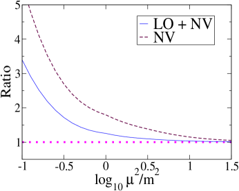
Figure 10: Comparison of form factors in instantaneous and non-instantaneous cases. The ratio Eq. (66) of form factors (LO + NV) is plotted versus $\log_{10}(\mu^{2}/m^{2})$ at fixed $\zeta=0.707$. Additionally the ratio Eq. (67) of non-valence contributions to the form factor (NV) is plotted. For $\mu^{2}\gg m^{2},M^{2}$, the non-instantaneous contributions becomes approximately instantaneous.

Lastly we remark that all of this is analytically clear: having eliminated different $\mu^{2}$ dependence hidden in $\psi$ and $\phi$, expressions for form factors in the instantaneous and non-instantaneous cases are identical to leading order in $1/\mu^{2}$, i.e. $\delta J^{+}_{A},\delta J^{+}_{B},\delta J^{+}_{C}\sim 1/\mu^{4}$ while the remaining non-valence contributions $\delta J^{+}_{D},\delta J^{+}_{E}$ match up with $\delta J^{+}_{1}$ and $\delta J^{+}_{2}$, respectively, to $1/\mu^{2}$.

Of course we have demonstrated the replacement of non-wave function vertices only to first order in perturbation theory. Schematically, we have required

$$|V-V_{o}|\ll|V(G-\operatorname{\tilde{G}})V|.$$ (68)

This is merely the condition that corrections to $V_{o}$ from finite $\mu^{2}$ are larger than second-order corrections from the reduction scheme in Eq. (45). Quantitatively this condition translates to $m/4\pi\mu\ll\alpha$. If this condition is met, the leading corrections are all of the form $V-V_{o}$ and the instantaneous model becomes the ladder model (and non-wave function vertices disappear when calculating the form factor). When the condition is not met, but holds to $[V(G-\operatorname{\tilde{G}})]^{2}V$, say, we must work up to second order in the reduction scheme and use the second Born approximation. We do not pursue this lengthy endeavor here, since for the non-instantaneous case $\gamma(x|M^{2})\propto\theta[x(1-x)]$ necessarily excludes non-wave function contributions in time-ordered perturbation theory. In fact at any order in time-ordered perturbation theory we expect to find a complete expression for the form factor in terms of Fock component overlaps devoid of non-wave function vertices, crossed interactions, etc.

V Summary

Above we investigate current matrix elements in the light-front Bethe-Salpeter formalism. First we present the issue of non-wave function vertices by taking up the common assumptions of light-front constituent quark models. By calculating the form factor in frames where $\zeta\neq 0$, Lorentz invariance mandates contribution from the vertex function’s poles. Quark models which neglect these residues and postulate a form for the wave function are assuming not only a pole-free vertex, but a vertex independent of light-front energy. These assumptions are very restrictive.

This leads us formally to investigate instantaneous and non-instantaneous contributions to wave functions and form factors necessitating the reduction formalism Eq. (25). We provide an intuitive interpretation for the light-front reduction, namely it is a procedure for approximating the poles of the Bethe-Salpeter vertex function. This procedure consists of covariant iterations followed by an instantaneous approximation cf Eq. (28), where the auxiliary Green’s function $\operatorname{\tilde{G}}$ enables the instantaneous approximation, see Eq. (26). In order to calculate form factors in the reduction formalism, we construct the gauge invariant current Eq. (35).

Using the ladder model (38) and an instantaneous approximation (44) we compare the calculation of wave functions and form factors in the light-front reduction scheme. Calculation of form factors is dissimilar for the two cases. In the ladder model, which is non-instantaneous, non-wave function vertices are excluded in time-ordered perturbation theory. For the instantaneous model, however, contribution from crossed interactions is required. Moreover, these instantaneous contributions derived are identical in form to non-wave function vertices used in constituent quark models. As a crucial check on our results, we take the limit $\mu^{2}\gg m^{2},M^{2}$ for which the ladder model becomes approximately instantaneous. In this limit, calculation of the form factors for the two models is identical.

The net result is an explicit proof, for $(1+1)$ dimensions, that non-wave function vertices are replaced by contributions form higher Fock states if the interactions between particles are not instantaneous. We call this a replacement theorem. The analysis relies on general features of the pole structure of the Bethe-Salpeter equation in light-front time-ordered perturbation theory. Therefore it is trivial to extend the theorem to $(3+1)$ dimensions. The real question which remains is whether or not the interaction between light quarks can be approximated as instantaneous. We intend to learn how to use experimental data to answer this question.

- (1) P. A. M. Dirac, Rev. Mod. Phys. 21, 392 (1949).
- (2) H. Leutwyler and J. Stern, Annals Phys. 112, 94 (1978).
- (3) G. P. Lepage and S. J. Brodsky, Phys. Rev. D 22, 2157 (1980).
- (4) S. J. Brodsky, H. C. Pauli and S. S. Pinsky, Phys. Rept. 301, 299 (1998).
- (5) J. Carbonell, B. Desplanques, V. A. Karmanov and J. F. Mathiot, Phys. Rept. 300, 215 (1998).
- (6) G. A. Miller, Prog. Part. Nucl. Phys. 45, 83 (2000).
- (7) N. E. Ligterink and B. L. Bakker, Phys. Rev. D 52, 5954 (1995); 5917 (1995).
- (8) J. H. Sales, T. Frederico, B. V. Carlson and P. U. Sauer, Phys. Rev. C 61, 044003 (2000); 63, 064003 (2001).
- (9) B. C. Tiburzi and G. A. Miller, hep-ph/0205109.
- (10) X.-D. Ji, J. Phys. G 24, 1181 (1998); A. V. Radyushkin, hep-ph/0101225; K. Goeke, M. V. Polyakov and M. Vanderhaeghen, Prog. Part. Nucl. Phys. 47, 401 (2001).
- (11) B. C. Tiburzi and G. A. Miller, hep-ph/0210305.
- (12) S. J. Brodsky, M. Diehl and D. S. Hwang, Nucl. Phys. B 596, 99 (2001); M. Diehl, T. Feldmann, R. Jakob and P. Kroll, Nucl. Phys. B 596, 33 (2001).
- (13) B. L. Bakker and C.-R. Ji, Phys. Rev. D 62, 074014 (2000).
- (14) M. B. Einhorn, Phys. Rev. D 14, 3451 (1976); M. Burkardt, Phys. Rev. D 62, 094003 (2000).
- (15) C.-R. Ji and H.-M. Choi, Phys. Lett. B 513, 330 (2001);
- (16) B. C. Tiburzi and G. A. Miller, Phys. Rev. D 65, 074009 (2002).
- (17) C. W. Hwang, Phys. Lett. B 530, 93 (2002).
- (18) J. P. B. C. de Melo, H. W. Naus and T. Frederico, Phys. Rev. C 59, 2278 (1999); J. P. B. C. de Melo, T. Frederico, E. Pace and G. Salmè, Nucl. Phys. A 707, 399 (2002).
- (19) W. Jaus, Phys. Rev. D 60, 054026 (1999).
- (20) N. B. Demchuk, I. L. Grach, I. M. Narodetski and S. Simula, Phys. Atom. Nucl. 59, 2152 (1996); I. L. Grach, I. M. Narodetsky and S. Simula, Phys. Lett. B 385, 317 (1996); C. Y. Cheung, C. W. Hwang and W. M. Zhang, Z. Phys. C 75, 657 (1997).
- (21) J. S. Schwinger, Proc. Nat. Acad. Sci. 37, 452 (1951); M. Gell-Mann and F. Low, Phys. Rev. 84, 350 (1951); E. E. Salpeter and H. A. Bethe, Phys. Rev. 84, 1232 (1951).
- (22) S. Weinberg, Phys. Rev. 150, 1313 (1966).
- (23) S. D. Drell and T. Yan, Phys. Rev. Lett. 24, 181 (1970); G. B. West, Phys. Rev. Lett. 24, 1206 (1970).
- (24) R. M. Woloshyn and A. D. Jackson, Nucl. Phys. B 64, 269 (1973).
- (25) F. Gross and D. O. Riska, Phys. Rev. C 36, 1928 (1987).
- (26) A. N. Kvinikhidze and B. Blankleider, Phys. Rev. C 60, 044003 (1999); 044004 (1999).
- (27) M. Sawicki and L. Mankiewicz, Phys. Rev. D 37 (1988) 421; L. Mankiewicz and M. Sawicki, Phys. Rev. D 40, 3415 (1989).