Traces of nonextensivity in particle physics due to fluctuations

Abstract

We present a short review of traces of nonextensivity in particle physics due to fluctuations.

1 Introduction: connection of fluctuations and nonextensivity

Both the notion of fluctuations and that of nonextensivity are nowdays widely known, albeit mostly in the fields of research only indirectly connected with particle physics. Both turns out to be very fruitful and interesting and this is clearly demonstrated by all other lectures given at this workshop (see especially [1, 2]).

This lecture will be devoted to the case in which evident nonextensivity of some expressions originate in intrinsic fluctuations in the system under consideration (the origin of which is usually not yet fully understood). The best introduction to this problem is provided by the observation that in some cosmic ray data (like depth distribution of starting points of cascades in Pamir lead chamber [13]) one observes clear deviations from the naively expected exponential distributions of some variables which are evidently better fitted by the power-like formulas:

$$\frac{dN}{dh}\,=\,{\rm const}\cdot\exp\left(\,-\,\frac{h}{\lambda}\,\right)\Rightarrow{\rm const}\cdot\left[1\,-\,(1-q)\frac{h}{\lambda}\right]^{\frac{1}{1-q}}.$$ (1)

Here $N$ denotes the number of counts at depth $h$ (cf. [13] for details). Whereas in [13] we have proposed as explanation a possible fluctuations of the mean free path $\lambda$ in eq. (1) characterised by relative variance $\omega\,=\,\frac{\left(\langle\sigma^{2}\rangle-\langle\sigma\rangle^{2}\right)}{\langle\sigma\rangle^{2}}\,\geq\,0.2$, in [3] the same data were fitted by power-like (Lévy type) formula as above keeping $\lambda$ fixed and setting $q=1.3$. In this way we have learned about Tsallis statistics and Tsallis nonextensive entropy and distributions. By closer inspection of the above example we have been able to propose a new physical meaning of the nonextensivity parameter $q$, as a measure of intrinsic fluctuations in the system [4, 5]. Fluctuations are therefore proposed as a new source of nonextensivity which should be added [14] to the previously known and listed in literature sources of the nonextensivity (like long-range correlations, memory effects or fractal-like structure of the corresponding phases space [2]) .

To demonstrate this conjecture let us notice that for $q>1$ case, where $\varepsilon\in(0,\infty)$, one can write a kind of Mellin transform (here $\alpha=\frac{1}{q-1}$) [5]:

$$\left(1\,+\,\frac{\varepsilon}{\lambda_{0}}\,\frac{1}{\alpha}\right)^{-a}\, = \,\frac{1}{\Gamma(\alpha)}\,\int^{\infty}_{0}\,d\eta\,{\eta}^{\alpha-1}\,\exp\left[-\eta\,\left(1\,+\,\frac{\varepsilon}{\lambda_{0}}\,\frac{1}{\alpha}\right)\right]$$ (2)

$$= \,\int^{\infty}_{0}\,\exp\left(-\frac{\varepsilon}{\lambda}\right)\,f_{q>1}\left(\frac{1}{\lambda}\right)\,d\left(\frac{1}{\lambda}\right)\,,$$

where $f_{q>1}(1/\lambda)$ is given by the following gamma distribution:

$$f_{q>1}\left(\frac{1}{\lambda}\right)\,=\,f_{q>1}\left(\frac{1}{\lambda},\frac{1}{\lambda_{0}}\right)\,=\,\frac{\mu}{\Gamma(\alpha)}\,\left(\frac{\mu}{\lambda}\right)^{\alpha-1}\,\exp\left(-\frac{\mu}{\lambda}\right)$$ (3)

with $\mu=\alpha\lambda_{0}$ and with mean value and variation in the form:

$$\left\langle\frac{1}{\lambda}\right\rangle\,=\,\frac{1}{\lambda_{0}}\qquad{\rm and}\qquad\left\langle\left(\frac{1}{\lambda}\right)^{2}\right\rangle\,-\,\left\langle\frac{1}{\lambda}\right\rangle^{2}\,=\,\frac{1}{\alpha\,\lambda_{0}^{2}}.$$ (4)

For the $q<1$ case $\varepsilon$ is limited to $\varepsilon\in[0,\lambda_{0}/(1-q)]$. Proceeding in the same way as before (but with $\alpha^{\prime}=-\alpha=\frac{1}{1-q}$) one gets:

$$\left[1\,-\,\frac{\varepsilon}{\alpha^{\prime}\lambda_{0}}\right]^{\alpha^{\prime}}\, = \,\frac{1}{\Gamma(\alpha^{\prime})}\,\int^{\infty}_{0}\,d\eta\,\eta^{\alpha^{\prime}-1}\,\exp\left[-\eta\,\left(1\,+\,\frac{\varepsilon}{\alpha^{\prime}\lambda_{0}-\varepsilon}\right)\right]$$ (5)

$$= \,\int^{\infty}_{0}\,\exp\left(-\frac{\varepsilon}{\lambda}\right)\,f_{q<1}\left(\frac{1}{\lambda}\right)\,d\left(\frac{1}{\lambda}\right)\,,$$

where $f_{q<1}(1/\lambda)$ is given by the same gamma distribution as in (3) but this time with $\alpha\rightarrow\alpha^{\prime}$ and $\mu=\mu(\varepsilon)=\alpha^{\prime}\lambda_{0}-\varepsilon$. Contrary to the $q>1$ case, this time the fluctuations depend on the value of the variable in question, i.e., the mean value and variance are now both $\varepsilon$-dependent:

$$\left\langle\frac{1}{\lambda}\right\rangle\,=\,\frac{1}{\lambda_{0}-\frac{\varepsilon}{\alpha^{\prime}}}\qquad{\rm and}\qquad\left\langle\left(\frac{1}{\lambda}\right)^{2}\right\rangle\,-\,\left\langle\frac{1}{\lambda}\right\rangle^{2}\,=\,\frac{1}{\alpha^{\prime}}\cdot\frac{1}{\left(\lambda_{0}-\frac{\varepsilon}{\alpha^{\prime}}\right)^{2}}.$$ (6)

However, in both cases the relative variances,

$$\omega\,=\,\frac{\left\langle\left(\frac{1}{\lambda}\right)^{2}\right\rangle\,-\,\left\langle\frac{1}{\lambda}\right\rangle^{2}}{\left\langle\frac{1}{\lambda}\right\rangle^{2}}\,=\,\left\{\begin{array}[]{c}\frac{1}{\alpha}\\ \\ \frac{1}{\alpha^{\prime}}\end{array}\right\}\,=\,\left\{\begin{array}[]{c}q-1\\ \\ 1-q\end{array}\right\}\,,$$ (7)

remain $\varepsilon$-independent and depend only on the parameter $q$ . It means therefore that [4, 5] (at least for the fluctuations distributed according to gamma distribution)

$$L=\exp\left(-\frac{x}{\lambda_{0}}\right)~{}~{}\Rightarrow~{}~{}L_{q}=\exp_{q}\left(-\frac{x}{\lambda_{0}}\right)=\left\langle\exp\left(-\frac{x}{\lambda}\right)\right\rangle,$$ (8)

with $q=1\,\pm\,\omega$ for $q>1~{}(+)$ and $q<1~{}(-)$, i.e., there is connection between the measure of fluctuations $\omega$ and the measure of nonextensivity $q$ (it has been confirmed recently in [14]).

2 Where are the fluctuations coming from?

2.1 Generalities

The proposed interpretation of the parameter $q$ leads immediately to the following question: why and under what circumstances it is the gamma distribution that describes fluctuations of the parameter $\lambda$? To address this question let us write the usual Langevin equation for the stochastic variable $\lambda$ [4, 5]:

$$\frac{d\lambda}{dt}\,+\,\left[\frac{1}{\tau}\,+\,\xi(t)\right]\,\lambda\,=\,\phi\,=\,{\rm const}\,>\,0.$$ (9)

with damping constant $\tau$ and with source term $\phi$, different for the two cases considered, namely:

$$\phi=\phi_{q<1}\,=\,\frac{1}{\tau}\left(\lambda_{0}-\frac{\varepsilon}{\alpha^{\prime}}\right)\qquad{\rm whereas}\qquad\phi=\phi_{q>1}=\frac{\lambda_{0}}{\tau}.$$ (10)

For the usual stochastic processes defined by the white gaussian noise form of $\xi(t)$ one obtains the following Fokker-Plank equation for the distribution function of the variable $\lambda$

$$\frac{df(\lambda)}{dt}\,=\,-\,\frac{\partial}{\partial\lambda}K_{1}\,f(\lambda)\,+\,\frac{1}{2}\,\frac{\partial^{2}}{\partial\lambda^{2}}K_{2}\,f(\lambda),$$ (11)

where the intensity coefficients $K_{1,2}$ are defined by eq.(9) and are equal to [4, 5]:

$$K_{1}(\lambda)\,=\,\phi\,-\,\frac{\lambda}{\tau}\,+\,D\,\lambda\qquad{\rm and}\qquad K_{2}(\lambda)\,=\,2\,D\,\lambda^{2}.$$ (12)

From it we get the following expression for the distribution function of the variable $\lambda$:

$$f(\lambda)\,=\,\frac{c}{K_{2}(\lambda)}\,\exp\left[\,2\,\int^{\lambda}_{0}d\lambda^{\prime}\,\frac{K_{1}(\lambda^{\prime})}{K_{2}(\lambda^{\prime})}\,\right]$$ (13)

which is, indeed, a gamma distribution (3) in variable $1/\lambda$, with the constant $c$ defined by the normalization condition, $\int^{\infty}_{0}d(1/\lambda)f(1/\lambda)=1$, and depending on two parameters: $\mu(\varepsilon)\,=\,\frac{\phi_{q}(\varepsilon)}{D}$ and $\alpha_{q}\,=\,\frac{1}{\tau\,D}$ with $\phi_{q}=\phi_{q>1,q<1}$ and $\alpha_{q}=(\alpha,\alpha^{\prime})$ for, respectively, $q>1$ and $q<1$. This means that we have obtained eqs.(7) with $\omega=\frac{1}{\tau D}$ and, therefore, the parameter of nonextensivity $q$ is given by the parameter $D$ and by the damping constant $\tau$ describing the white noise.

2.2 Temperature fluctuations

The above discussion rests on the stochastic equation (9). Therefore the previously asked question is not yet fully answered but can be refrazed in the following way: can one point the possible physical situation where such fluctuations could be present in the realm of particle physics? Our proposition to answer it is to identify $\lambda=T$, i.e., to concentrate on the possibility of fluctuations of temperature widely discussed in the literature in different contexts [15]. In all cases of interest to us temperature $T$ is variable encountered in statistical descriptions of multiparticle collision processes [16]. Our reasoning goes then as follows: Suppose that we have a thermodynamic system, in a small (mentally separated) part of which the temperature fluctuates with $\Delta T\sim T$. Let $\lambda(t)$ describe stochastic changes of the temperature in time. If the mean temperature of the system is $\langle T\rangle=T_{0}$ then, as result of fluctuations in some small selected region, the actual temperature equals $T^{\prime}=T_{0}-\tau\xi(t)T$ and the inevitable exchange of heat between this selected region and the rest of the system leads to the process of equilibration of the temperature which is described by the following equation of the type of eq. (9) [17] :

$$\frac{\partial T}{\partial t}\,-\,\frac{1}{\tau}\,(T^{\prime}\,-\,T)\,+\,\Omega_{q}=0$$ (14)

(here $\Omega_{q<1}=\frac{\varepsilon}{\tau\alpha^{\prime}}$ and $\Omega_{q>1}=0$). In this way we have demonstrated that eq. (9) can, indeed, be used in statistical models of multiparticle production as far as they allow the $q$-statistic as their basis.

The $q<1$ case requires a few additional words of explanation. Notice the presence of the internal heat source, which is dissipating (or transfering) energy from the region where (due to fluctuations) the temperature $T$ is higher to colder ones. It could be any kind of convection-type flow of energy; for example, it could be connected with emission of particles from that region. The heat release given by $\varepsilon/(\tau\alpha^{\prime})$ depends on $\varepsilon$ (but it is only a part of $\varepsilon$ that is released). In the case of such energy release (connected with emission of particles) there is additional cooling of the whole system. If this process is sufficiently fast, it could happen that there is no way to reach a stationary distribution of temperature (because the transfer of heat from the outside can be not sufficient for the development of the state of equilibrium). On the other hand (albeit this is not our case here) in the reverse process we could face the ”heat explosion” situation (which could happen if the velocity of the exothermic burning reaction grows sufficiently fast; in this case because of nonexistence of stationary distribution we have fast nonstationary heating of the substance and acceleration of the respective reaction).

The most interesting example of the possible existence of such fluctuations is the trace of power like behaviour of the transverse momentum distribution in multiparticle production processes encountered in heavy ion collisions [18, 6]. Such collisions are of special interest because they are the only place where new state of matter, the Quark Gluon Plasma, can be produced [16]. Transverse momentum distributions are believed to provide information on the temperature $T$ of reaction, which is given by the inverse slope of $dN/dp_{T}$, if it is exponential one. If it is not, question arises what we are really measuring. One explanation is the possible flow of the matter, the other, which we shall follow here, is the nonextensivity (or rather fluctuations leading to it). Namely, as was discussed in detail in [18] the extreme conditions of high density and temperature occuring in ultrarelativistic heavy ion collisions can invalidate the usual BG approach and lead to $q>1$, i.e., to

$$\frac{dN(p_{T})}{dp_{T}}={\rm const}\cdot\left[1\,-(1-q)\frac{\sqrt{m^{2}+p^{2}_{T}}}{T}\right]^{\frac{1}{1-q}}.$$ (15)

Here $m$ is the mass of produced particle and $T$ is, for the $q=1$ case, the temperature of the hadronic system produced. Although very small ($|q-1|\sim 0.015$) this deviation, if interpreted according to eq. (8)), leads to quite large relative fluctuations of temperature existing in the nuclear collisions, $\Delta T/T\simeq 0.12$. It is important to stress that these are fluctuations existing in small parts of hadronic system in respect to the whole system rather than of the event-by-event type for which, $\Delta T/T=0.06/\sqrt{N}\rightarrow 0$ for large $N$ (cf. [7] for relevant references). Such fluctuations are potentially very interesting because they provide direct measure of the total heat capacity $C$ of the system,

$$\frac{\sigma^{2}(\beta)}{\langle\beta\rangle^{2}}\,=\,\frac{1}{C}\,=\,\omega\,=\,q-1\,,$$ (16)

($\beta=\frac{1}{T}$) in terms of $\omega=q-1$. Therefore, measuring both the temperature of reaction $T$ and (via nonextensivity $q\neq 1$) its total heat capacity $C$, one can not only check whether an approximate thermodynamics state is formed in a single collision but also what are its theromdynamical properties (especially in what concerns the existence and type of the possible phase transitions [7]).

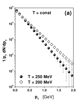
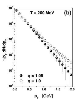
Figure 1: $(a)$ Normal exponential $p_{T}$ distributions (i.e., $q=1$) for $T=200$ MeV (black symbols) and $T=250$ MeV open symbols). $(b)$ Typical event from central $Pb+Pb$ at $E_{beam}=3~{}A\cdot$TeV (cf. text for other details) for $=200$ MeV for $q=1$ (black symbols) exponential dependence and $q=1.05$ (open symbols).

To observe such fluctuations an event-by-event analysis of data is needed [7]. Two scenarios must be checked: $(a)$ $T$ is constant in each event but because of different initial conditions it fluctuates from event to event and $(b)$ $T$ fluctuates in each event around some mean value $T_{0}$. Fig. 1 shows typical event obtained in simulations performed for central $Pb+Pb$ collisions taking place for beam energy equal $E_{beam}=3~{}A\cdot$TeV in which density of particles in central region (defined by rapidity window $-1.5<y<1.5$) is equal to $\frac{dN}{dy}=6000$ (this is the usual value given by commonly used event generators [20]). In case $(a)$ in each event one expects exponential dependence with $T=T_{event}$ and possible departure from it would occur only after averaging over all events. It would reflect fluctuations originating from different initial conditions for each particular collision. This situation is illustrated in Fig. 1a where $p_{T}$ distributions for $T=200$ MeV (black symbols) and $T=250$ MeV (open symbols) are presented. Such values of $T$ correspond to typical uncertainties in $T$ expected at LHC accelerator at CERN. Notice that both curves presented here are straight lines. In case $(b)$ one should observe departure from the exponential behaviour already on the single event level and it should be fully given by $q>1$. It reflects situation when, due to some intrinsically dynamical reasons, different parts of a given event can have different temperatures [4, 5]. In Fig. 1b black symbols represent exponential dependence obtained for $T=200$ MeV (the same as in Fig. 1a), open symbols show the power-like dependence as given by (15) with the same $T$ and with $q=1.05$ (notice that the corresponding curve bends slightly upward here). In this typical event we have $\sim 18000$ secondaries, i.e., practically the maximal possible number. Notice that points with highest $p_{T}$ correspond already to single particles. As one can see, experimental differentiation between these two scenarios will be very difficult, although not totally impossible. On the other hand, if successful it would be very rewarding - as we have stressed before.

One should mention at this point that to the same cathegory of fluctuating temperature belongs also attempt [21] to fit energy spectra in both the longitudinal and transverse momenta of particles produced in the $e^{+}e^{-}$ annihilation processes at high energies, novel nonextensive formulation of Hagedorn statistical model of hadronization process [19, 14] and description of single particle spectra [8, 12].

2.3 Nonexponential decays

Another hint for intrinsic fluctuations operating in the physical system could be the known phenomenon of nonexponential decays [9]. Spontaneous decays of quantum-mechanical unstable systems cannot be described by the pure exponential law (neither for short nor for long times) and survival time probability is $P(t)\propto t^{-\delta}$ instead of exponential one. It turns out [9] that by using random matrix approach, such decays can emerge in a natural way from the possible fluctuations of parameter $\gamma=1/\tau$ in the exponential distribution $P(t)=\exp(-\gamma t)$. Namely, in the case of multichannel decays (with $\nu$ channels of equal widths involved) one gets fluctuating widths distributed according to gamma function

$$P_{\nu}(\gamma)=\frac{1}{\Gamma\left(\frac{\nu}{2}\right)}\left(\frac{\nu}{2<\gamma>}\right)\left(\frac{\nu\gamma}{2<\gamma>}\right)^{\frac{\nu}{2}-1}\exp\left(-\frac{\nu\gamma}{2<\gamma>}\right)$$ (17)

and strength of their fluctuations is given by relative variance $\frac{\left\langle(\gamma\,-\,<\gamma>)^{2}\right\rangle}{<\gamma>^{2}}\,=\,\frac{2}{\nu}$, which decreases with increasing $\nu$. According to [4], it means therefore that, indeed,

$$L_{q}(t,\tau_{0})=\frac{2-q}{\tau_{0}}\,\left[1\,-\,(1-q)\frac{t}{\tau_{0}}\right]^{\frac{1}{1-q}},$$ (18)

with the nonextensivity parameter equal to $q=1+\frac{2}{\nu}$.

3 Summary

There is steadily growing evidence that some peculiar features observed in particle and nuclear physics (including cosmic rays) can be most consistently explained in terms of the suitable applications of nonextensive statistic of Tsallis. Here we were able to show only some selected examples, more can be found in [5, 11]. However, there is also some resistance towards this idea, the best example of which is provided in [22]. It is shown there that mean multiplicity of neutral mesons produced in $p-\bar{p}$ collisions as a function of their mass (in the range from $m_{\eta}=0.55$ GeV to $M_{\Upsilon}=9.5$ GeV) and the transverse mass $m_{T}$ spectra of pions (in the range of $m_{T}\simeq 1\div 15$ GeV), both show a remarkable universal behaviour following over $10$ orders of magnitude the same power law function $C\cdot x^{-P}$ (with $x=m$ or $x=m_{T}$) with $P\simeq 10.1$ and $P\simeq 9.6$, respectively. In this work such a form was just postulated whereas it emerges naturally in $q$-statistics with $q=1+1/P\sim 1.1$ (quite close to results of [21]). We regard it as new, strong imprint of nonextensivity present in multiparticle production processes (the origin of which remains, however, to be yet discovered). This interpretation is additionally supported by the fact that in both cases considered in [22] the constant $c$ is the same. Apparently there is no such phenomenon in $AA$ collisions which has simple and interesting explanation: in nuclear collisions volume of interaction is much bigger what makes the heat capacity $C$ also bigger. This in turn, cf. eq.(16), makes $q$ smaller. On should then, indeed, expect that $q_{hadronic}>>q_{nuclear}$, as observed.

As closing remark let us point out the alternate way of getting nonextensive (i.e., with $q\neq 1$) distributions for thermal models (cf. our remarks in [3] and the more recent ideas presented in [23]). Notice that if we allow for the temperature $T$ to be energy $E$ dependent, i.e., that $T=T(E)=T_{0}+a\cdot(E-\tilde{E})$ (with $a=1/C_{V}$) then the usual equation on the probability $P(E)$ that a system $A$ (interacting with the heat bath $A^{\prime}$ with temperature $T$) has energy $E$,

$$d\ln[P(E)]\sim-dE/T\qquad\Longrightarrow\qquad P(E)\sim\exp\left(-\frac{E}{T}\right)$$ (19)

becomes

$$d\ln P(E)\sim\frac{1}{T_{0}+a(E-\tilde{E})}dE\quad\Longrightarrow\quad P(E)\sim\left[1-(1-q)\frac{E-\tilde{E}}{T_{0}}\right]^{\frac{1}{1-q}}$$ (20)

with $q=1+a$. This approach could then find its possible application to studies of fluctuations on event-by-event basis [24] (with all reservations expressed in [25] accounted for).

References

- [1] In what concerns fluctuations see A.Białas, these proceedings (and references therein).
- [2] In what concerns nonextensivity see C.Tsallis, these proceedings and references therein. In particular see Nonextensive Statistical Mechanics and its Applications, S.Abe and Y.Okamoto (Eds.), Lecture Notes in Physics LPN560, Springer (2000).
- [3] G.Wilk and Z.Włodarczyk, Nucl. Phys. B (Proc. Suppl.) A75 (1999) 191.
- [4] G.Wilk and Z.Włodarczyk, Phys. Rev. Lett. 84 (2000) 2770.
- [5] G.Wilk and Z.Włodarczyk, Chaos, Solitons and Fractals 13/3 (2001) 581.
- [6] O.V.Utyuzh, G.Wilk and Z.Włodarczyk, J. Phys. G26 (2000) L39.
- [7] O.V.Utyuzh, G.Wilk and Z.Włodarczyk, How to observe fluctuating temperature?, hep-ph/0103273.
- [8] F.S.Navarra, O.V.Utyuzh, G.Wilk and Z.Włodarczyk, Nuovo Cim. 24C (2001) 725.
- [9] G.Wilk and Z.Włodarczyk, Phys. Lett. A290 (2001) 55.
- [10] M.Rybczyński, Z.Włodarczyk and G.Wilk, Nucl. Phys. (Proc. Suppl.) B97 (2001) 81.
- [11] G.Wilk and Z.Włodarczyk, Physica A305 (2002) 227.
- [12] M.Rybczyński, Z.Włodarczyk and G.Wilk; Rapidity spectra analysis in terms of non-extensive statistic approach; Presented at the XII ISVHECRI, CERN, 15-20 July 2002; hep-ph/0206157.
- [13] G.Wilk and Z.Włodarczyk, Phys. Rev. D50 (1994) 2318.
- [14] C.Beck, Physica A305 (2002) 209; Phys. Rev. Lett. 87 (2001) 180601 and Europhys. Lett. 57 (2002) 329.
- [15] L.D.Landau, I.M.Lifschitz, Course of Theoretical Physics: Statistical Physics, Pergmon Press, New York 1958. See also: L.Stodolsky, Phys. Rev. Lett. 75 (1995) 1044. For different aspects of fluctuations see: T.C.P.Chui, D.R.Swanson, M.J.Adriaans, J.A.Nissen and J.A.Lipa, Phys. Rev. Lett. 69 (1992) 3005; C.Kittel, Physics Today 5 (1988) 93; B.B.Mandelbrot, Physics Today 1 (1989) 71; H.B.Prosper, Am. J. Phys. 61 (1993) 54; G.D.J.Phillires, Am. J. Phys. 52 (1984) 629. For particle physics aspects see: E.V.Shuryak, Phys. Lett. B423 (1998) 9 and S.Mrówczyński, Phys. Lett. B430 (1998) 9.
- [16] See, for example, proceedings of QM2001, eds. T.J.Hallman et al., Nucl. Phys. A698 (2002) and references therein.
- [17] L.D.Landau and I.M.Lifschitz, Course of Theoretical Physics: Hydrodynamics, Pergamon Press, New York 1958 or Course of Theoretical Physics: Mechanics of Continous Media, Pergamon Press, Oxford 1981.
- [18] W.M.Alberico, A.Lavagno and P.Quarati, Eur. Phys. J. C12 (2000) 499 and Nucl. Phys. A680 (2001) 94c.
- [19] C.Beck, Physica A286 (2000) 164.
- [20] K.J.Escola, see [16] p. 78.
- [21] I.Bediaga, E.M.F.Curado and J.M.de Miranda, Physica A286 (2000) 156.
- [22] M.Gaździcki and M.I.Gorenstein, Phys. Lett. B517 (2001) 250.
- [23] M.P.Almeida, Physica A300 (2001) 424.
- [24] R.Korus, St.Mrówczyński, M.Rybczyński and Z.Włodarczyk, Phys. Rev. C64 (2001) 054908.
- [25] M.Rybczyński, Z.Włodarczyk and G.Wilk, Phys. Rev. C64 (2001) 027901.