Radiative Corrections to Double Dalitz Decays:
Effects on Invariant Mass Distributions and Angular Correlations

Abstract

We review the theory of meson decays to two lepton pairs, including the cases of identical as well as non–identical leptons, as well as CP–conserving and CP–violating couplings. A complete lowest–order calculation of QED radiative corrections to these decays is discussed, and comparisons of predicted rates and kinematic distributions between tree–level and one–loop–corrected calculations are presented for both $\pi^{0}$ and $K^{0}$ decays.

I Background

Meson decays to two photons should exhibit interesting correlations between the photon polarizationsYang (1950). Although existing particle detectors cannot measure photon polarizations directly, it has long been known that the polarization correlations can be measured indirectly by studying angular correlations in the related double Dalitz decaysKroll and Wada (1955) in which both photons undergo internal conversion to a lepton pair. More recently, it has been pointed outUy (1991) that a detailed study of these correlations can be used to determine the relative amount of two possible meson–$\gamma\gamma$ couplings (one CP–conserving and one CP–violating for mesons that are CP eigenstates) that can contribute to this process.

Dalitz and double Dalitz decays are also of interest because they can be exploited to perform a measurement of the electromagnetic form factor of the decaying meson — that is, how the meson couples to one real and one virtual photon (Dalitz decay) or two virtual photons (double Dalitz) depends on the $q^{2}$ values of the photon(s). An accurate knowledge of this form factor is essential, for example, to calculate the so–called long–distance contribution to the rare decay $K_{L}\to\mu^{+}\mu^{-}$. The short–distance contribution to this process, mediated by loops involving heavy quarks and massive vector bosons, is sensitive to the CKM matrix element $V_{td}$, but this contribution cannot be extracted from the accurate experimental measurement of the partial width unless the long–distance amplitude is precisely known.

The tree–level rates for several double Dalitz processes have been published in various formsKroll and Wada (1955); Hunt (1970); Miyazaki and Takasugi (1973); Uy (1991). The first experimental observation of a double Dalitz decay was published in 1962Plano et al. (1959); Samios et al. (1962). A total of 206 examples of the decay $\pi^{0}\to e^{+}e^{-}e^{+}e^{-}$ were observed by Samios in a sample of some 800,000 bubble chamber photographs. Based on the observed angular correlations, Samios was able to exclude the possibility that the $\pi^{0}$ was a scalar particle (with a CP–conserving decay) at the $3.3\sigma$ confidence level. His measurement of the branching ratio for that process remains the only one published to date.

Experimental observations of the much rarer kaon double Dalitz decays began to appear in the 1990’s. Several measurements have been made of the decay $K_{L}\to e^{+}e^{-}e^{+}e^{-}$Barr et al. (1991); Vagins et al. (1993); Akagi et al. (1993); Gu et al. (1994); Barr et al. (1995); Akagi et al. (1995); Alavi-Harati et al. (2001a), the most recent of which are based on several hundred observed events. The still rarer double Dalitz mode $K_{L}\to e^{+}e^{-}\mu^{+}\mu^{-}$ is particularly interesting because it is free of complications arising when there are two identical lepton pairs in the final state, and because it probes only the kinematic region in which one of the virtual photons has $q^{2}>4m_{\mu}^{2}$. The first example of this decay was reported in 1996Gu et al. (1996). In 2001 the KTeV experiment published a branching ratio based on a sample of 43 eventsAlavi-Harati et al. (2001b); most recently, KTeV has reported results from a combined sample of 132 events, including the earlier 43Hamm (2002).

Further experimental results on both $\pi^{0}\to e^{+}e^{-}e^{+}e^{-}$ and the two kaon decays are expected in the near future from the NA48 and KTeV experiments. As the statistics available to the experimenters increase, it will be necessary to have a more accurate theoretical description of these decays, incorporating the significant effects of QED radiative corrections. These corrections, discussed in this paper, have a significant impact on the extraction of both form factors and angular correlations from high–statistics data.

II Tree–Level Amplitudes

The most general CPT invariant interaction governing the transition of a spin–zero meson to two photons is

$$\mathcal{L}=\frac{-i}{4M}\left[\mathcal{F}_{P}\,\epsilon_{\mu\nu\rho\sigma}+\mathcal{F}_{S}\left(g_{\mu\rho}g_{\nu\sigma}-g_{\mu\sigma}g_{\nu\rho}\right)\right]F^{\mu\nu}F^{\rho\sigma}\phi,$$ (1)

where $\mathcal{F}_{P}$ and $\mathcal{F}_{S}$ are dimensionless form factors for a pseudoscalar and scalar coupling which may be momentum dependent, $F^{\mu\nu}$ is the electromagnetic field tensor, and $\phi$ is the field of a meson of mass $M$. The factor of $-i$ defines a phase convention in which the form factors will be real if CPT invariance holds and there are no absorptive decay amplitudes. It will be convenient to decompose the couplings into real and imaginary parts, and define them (up to an arbitrary overall phase $\Psi$) in terms of a mixing angle $\zeta$, and a phase difference $\delta$,

$$\mathcal{F}_{P} =g_{P}f_{P}(k_{1}^{2},k_{2}^{2})e^{i\Psi}=\tilde{g}f_{P}(k_{1}^{2},k_{2}^{2})\cos{\zeta}e^{i\Psi},$$ (2a)

$$\mathcal{F}_{S} =g_{S}f_{S}(k_{1}^{2},k_{2}^{2})e^{i\Phi}=\tilde{g}f_{S}(k_{1}^{2},k_{2}^{2})\sin{\zeta}e^{i\delta}e^{i\Psi},$$ (2b)

where $\tilde{g}^{2}=g_{P}^{2}+g_{S}^{2}$ and $\delta=\Phi-\Psi$. $f_{P}$ and $f_{S}$ are functions of the $k^{2}$ values of the two virtual photons and are normalized such that $f(0,0)=1$ for both couplings. In principle it is also possible for $\delta$ to depend on $k_{1}^{2}$ and $k_{2}^{2}$.

II.1 Two–Photon Decay

The two–photon partial width provides information about the coupling constant $\tilde{g}$ along with some constraints on the mixing angle $\zeta$ and phase difference $\delta$. The matrix element for the decay to two real photons with helicities $\lambda_{1}$ and $\lambda_{2}$ is

$$\begin{split}\mathcal{M}_{\lambda_{1}\lambda_{2}}=&\frac{2}{M}[\mathcal{F}_{P}\,\epsilon_{\mu\nu\rho\sigma}\\ &+\mathcal{F}_{S}(g_{\mu\rho}g_{\nu\sigma}-g_{\mu\sigma}g_{\nu\rho})]k_{1}^{\mu}\epsilon_{\lambda_{1}}^{*\nu}k_{2}^{\rho}\epsilon_{\lambda_{2}}^{*\sigma},\end{split}$$ (3)

where $k^{\mu}$ and $\epsilon^{\mu}$ are the momentum and polarization of a photon. The calculation of the two–photon couplings for photons of arbitrary mass is carried out in Appendix B. For real photons, the kinematic factors in the couplings reduce to $\lambda=z=1$ and $w=0$, and the momentum dependent functions $f_{P}$ and $f_{S}$ reduce to unity. Therefore, one has the following two contributions

$$\mathcal{M}_{++} =-M\tilde{g}\left(\sin{\zeta}e^{i\delta}-i\cos{\zeta}\right),$$ (4a)

$$\mathcal{M}_{--} =-M\tilde{g}\left(\sin{\zeta}e^{i\delta}+i\cos{\zeta}\right).$$ (4b)

The partial width is obtained by integrating $1/(2M)$ times the squared matrix element over the available phase space. The matrix element is a constant, so the integration results in a factor of $1/(16\pi)$. The partial widths for the two allowed helicity states are then

$$\Gamma_{++} =\frac{M\tilde{g}^{2}}{32\pi}\left(1-2\sin{\zeta}\cos{\zeta}\sin{\delta}\right),$$ (5a)

$$\Gamma_{--} =\frac{M\tilde{g}^{2}}{32\pi}\left(1+2\sin{\zeta}\cos{\zeta}\sin{\delta}\right).$$ (5b)

The decay rates to the two final states will be identical if either the phase difference between the two couplings is zero or one of the form factors is zero. In any case, the total rate is equal to $\Gamma_{\gamma\gamma}=M\tilde{g}^{2}/(16\pi)$. An experimental measure of the two–photon width then gives a value of $\tilde{g}$,

$$\tilde{g}=\sqrt{16\pi\Gamma_{\gamma\gamma}/M}.$$ (6)

II.2 Application to Neutral Pion and Kaon Decays

One can compute $\tilde{g}$ for the $\pi^{0}\to\gamma\gamma$, $K_{L}\to\gamma\gamma$, and $K_{S}\to\gamma\gamma$ decays using the current experimental valuesHagiwara et al. (2002) of the two–photon branching ratios along with the meson lifetimes and masses, with the results

$$\tilde{g}_{0} =(1.70\pm 0.06)\cdot 10^{-3},$$ (7a)

$$\tilde{g}_{L} =(8.75\pm 0.12)\cdot 10^{-10},$$ (7b)

$$\tilde{g}_{S} =(1.36\pm 0.11)\cdot 10^{-9}.$$ (7c)

It will be useful to define CP–even and CP–odd $\gamma\gamma$ states:

$$|(\gamma\gamma)_{\pm}\rangle=(|++\rangle\pm|--\rangle)/\sqrt{2}.$$ (8)

The matrix elements for $\pi^{0}\to\gamma\gamma$ are then given by

$$\langle(\gamma\gamma)_{+}|\ T\ |\pi^{0}\rangle =-i\sqrt{2}M_{\pi}\tilde{g}_{0}\sin\zeta_{0}e^{i\Phi_{0}},$$ (9a)

$$\langle(\gamma\gamma)_{-}|\ T\ |\pi^{0}\rangle =-\sqrt{2}M_{\pi}\tilde{g}_{0}\cos\zeta_{0}e^{i\Psi_{0}}.$$ (9b)

Similar expressions can be given for the $K_{1}$ and $K_{2}$ decay matrix elements with the 0 subscripts changed to 1 or 2 respectively and $M_{\pi}$ replaced by $M_{K}$. These expressions may be compared to those in Ref. Sehgal (1971) in which CP–violation observables for the $K\to\gamma\gamma$ decays were calculated. In that article Sehgal defines

$$\langle(\gamma\gamma)_{+}|\ T\ |K_{1}\rangle =\phantom{-i}c_{e}e^{i\rho_{e}},$$ (10a)

$$\langle(\gamma\gamma)_{-}|\ T\ |K_{1}\rangle =\phantom{-}ic_{o}e^{i\rho_{o}},$$ (10b)

$$\langle(\gamma\gamma)_{+}|\ T\ |K_{2}\rangle =-id_{e}e^{i\mu_{e}},$$ (10c)

$$\langle(\gamma\gamma)_{-}|\ T\ |K_{2}\rangle =\phantom{-i}d_{o}e^{i\mu_{o}}.$$ (10d)

In our notation we have

$$c_{e} =\phantom{-}\sqrt{2}M_{K}\tilde{g}_{1}\sin\zeta_{1},$$ (11a)

$$c_{o} =-\sqrt{2}M_{K}\tilde{g}_{1}\cos\zeta_{1},$$ (11b)

$$d_{e} =\phantom{-}\sqrt{2}M_{K}\tilde{g}_{2}\sin\zeta_{2},$$ (11c)

$$d_{o} =-\sqrt{2}M_{K}\tilde{g}_{2}\cos\zeta_{2}.$$ (11d)

The observable phase differences are given by $\delta_{1}=\rho_{e}-\rho_{o}$ and $\delta_{2}=\mu_{e}-\mu_{o}$.

The phases $\delta_{i}$ are observable only if CP is violated in $\gamma\gamma$ decays. As Sehgal noted in Ref. Sehgal (1971), the phase $\delta_{0}$ in $\pi^{0}$ decays should be very close to zero if CPT is conserved because the relevant absorptive amplitudes are of order $\alpha^{2}$. In the case of kaon decays, on–shell intermediate states such as $\pi\pi$ couple strongly so that the phases $\delta_{1}$ and $\delta_{2}$ may be large even if CPT is conserved.

II.3 Four–Lepton Decay

While the total two–photon decay rate provides information about the constant part of the form factors, the four–lepton rate can be utilized to probe both the momentum dependence of the form factors and the mixing of the couplings. The decay to four leptons may contain either two pairs of identical particles (e.g., $K_{L}\to e^{+}e^{-}e^{+}e^{-}$) or pairs of non–identical particles (e.g., $K_{L}\to e^{+}e^{-}\mu^{+}\mu^{-}$). The tree–level Feynman diagram for the decay is depicted in Fig. 1.

Figure 1: Double Dalitz Tree–Level Diagram.

If the final state does contain identical particles, then there is also an exchange diagram, as shown in Fig. 2.

Figure 2: Double Dalitz Exchange Diagram.

The matrix element is then the sum of the two diagrams $\mathcal{M}=\mathcal{M}_{1}+\mathcal{M}_{2}$ and its square is $|\mathcal{M}|^{2}=|\mathcal{M}_{1}|^{2}+|\mathcal{M}_{2}|^{2}+2\operatorname{Re}{(\mathcal{M}_{1}^{*}\mathcal{M}_{2})}$. The analysis presented in the rest of this section applies only to the direct contribution to the double Dalitz process. Appendix C gives an explicit expression for the interference term.

The matrix element for the direct contribution to the double Dalitz process can be written as

$$\mathcal{M}_{1}=H_{\mu\nu\rho\sigma}k_{1}^{\mu}\Pi^{\nu\alpha}\Gamma_{\alpha}k_{2}^{\rho}\Pi^{\sigma\beta}\Gamma_{\beta},$$ (12)

where $H$ is a two–photon coupling given by Eq. (94), $k$ is a photon momentum, $\Pi$ is the propagator for a photon of momentum $k$

$$\Pi^{\mu\nu}(k)=\frac{i}{k^{2}}\left(\sum_{\lambda}\epsilon_{\lambda}^{*\mu}\epsilon_{\lambda}^{\nu}-\hat{k}^{\mu}\hat{k}^{\nu}\right),$$ (13)

and $\Gamma$ is the fermion current for an electron of momentum $q$ and spin $r$ and positron of momentum $p$ and spin $s$

$$\Gamma^{\mu}(q,p;r,s)=-ie\bar{u}_{r}(q)\gamma^{\mu}v_{s}(p).$$ (14)

The sum in the propagator extends over the three helicity states and the term proportional to $k^{\mu}k^{\nu}$ vanishes when contracted with the current. The matrix element can then be cast as

$$\mathcal{M}_{1}=\sum_{\lambda_{1}\lambda_{2}}\mathcal{H}_{\lambda_{1}\lambda_{2}}L_{\lambda_{1}}L_{\lambda_{2}},$$ (15)

where $\mathcal{H}$ is one of the two–photon couplings given in Eqs. (96,97). The quantity $L$ contains all the lepton information and is equal to $L_{\lambda}=i\epsilon_{\lambda}^{\mu}\Gamma_{\mu}/k^{2}$.

The squared matrix element, summed over final state helicities can be expressed in terms of the five phase space variables $x_{12}$, $x_{34}$, $y_{12}$, $y_{34}$, and $\phi$ (defined in Appendix A). Focusing on the $\phi$ dependence, the squared amplitude is

$$\begin{split}\sum|\mathcal{M}_{1}|^{2}=\frac{2^{8}\pi^{2}\alpha^{2}\tilde{g}^{2}}{M^{2}w^{4}}&(A\sin^{2}\phi+B\cos^{2}\phi\\ &+C\sin\phi\cos\phi+D\sin\phi\\ &+E\cos\phi+F),\end{split}$$ (16)

where

$$A= w^{2}\{f_{P}^{2}\cos^{2}\zeta\lambda^{2}[1+(1-\lambda_{12}^{2}+y_{12}^{2})(1-\lambda_{34}^{2}+y_{34}^{2})]$$

$$\quad+f_{S}^{2}\sin^{2}\zeta z^{2}[2-\lambda_{12}^{2}-\lambda_{34}^{2}+y_{12}^{2}+y_{34}^{2}]\},$$ (17a)

$$B= w^{2}\{f_{S}^{2}\sin^{2}\zeta z^{2}[1+(1-\lambda_{12}^{2}+y_{12}^{2})(1-\lambda_{34}^{2}+y_{34}^{2})]$$

$$\quad+f_{P}^{2}\cos^{2}\zeta\lambda^{2}[2-\lambda_{12}^{2}-\lambda_{34}^{2}+y_{12}^{2}+y_{34}^{2}]\},$$ (17b)

$$C= 2f_{P}f_{S}\sin\zeta\cos\zeta\cos\delta\lambda zw^{2}$$

$$\quad\quad\times(\lambda_{12}^{2}-y_{12}^{2})(\lambda_{34}^{2}-y_{34}^{2}),$$ (17c)

$$D= 2f_{P}f_{S}\sin\zeta\cos\zeta\cos\delta\lambda w^{3}y_{1}y_{2}$$

$$\quad\quad\times\sqrt{(\lambda_{12}^{2}-y_{12}^{2})(\lambda_{34}^{2}-y_{34}^{2})},$$ (17d)

$$E= 2f_{S}^{2}\sin^{2}\zeta zw^{3}y_{12}y_{34}\sqrt{(\lambda_{12}^{2}-y_{12}^{2})(\lambda_{34}^{2}-y_{34}^{2})},$$ (17e)

$$F= f_{S}^{2}\sin^{2}\zeta w^{4}(1-y_{12}^{2})(1-y_{34}^{2}),$$ (17f)

where the kinematic variables $w$, $z$, and $\lambda$ are defined in Appendix A. Terms $A$ and $B$ arise from the diagonal pieces of the transverse part of the pseudoscalar and scalar couplings while term $F$ is due to the diagonal piece of the longitudinal part of the scalar coupling. Term $C$ is the interference between the transverse parts of the pseudoscalar and scalar couplings while terms $D$ and $E$ are due to interference between the longitudinal part of the scalar and the transverse parts of the pseudoscalar and scalar couplings respectively.

The partial width is obtained by integrating $1/(2M)$ times the square of the matrix element over the eight dimensional phase space (given in Appendix A). The integrals over $y_{ij}$ extend from $-\lambda_{ij}$ to $+\lambda_{ij}$ and can be done analytically. The differential partial width, normalized to the two–photon width and integrated over $y_{12}$ and $y_{34}$, is

$$\begin{split}\frac{1}{\Gamma_{\gamma\gamma}}\frac{d\Gamma_{1}}{d\phi}=\frac{\mathcal{S}\alpha^{2}}{3\pi^{3}}&[I_{1}\cos^{2}\zeta\sin^{2}\phi+I_{2}\sin^{2}\zeta\cos^{2}\phi\\ &+I_{3}\sin\zeta\cos\zeta\cos\delta\sin\phi\cos\phi\\ &+I_{4}\cos^{2}\zeta+(I_{5}+I_{6})\sin^{2}\zeta],\end{split}$$ (18)

where $\mathcal{S}$ is a symmetry factor which is $1/4$ for modes with identical particles and 1 otherwise.

Table 1: Results of numerical integrations over $x_{12}$ and $x_{34}$ assuming $f_{P}=f_{S}=1$.

Integral	$K_{L}\to ee\mu\mu$	$K_{L}\to\mu\mu\mu\mu$	$K_{L}\to eeee$	$\pi^{0}\to eeee$
$I_{1}$	0.10627	$2.977\cdot 10^{-6}$	14.146	7.2287
$I_{2}$	0.11147	$1.149\cdot 10^{-5}$	14.201	7.2838
$I_{3}$	0.21713	$1.120\cdot 10^{-5}$	28.343	14.509
$I_{4}$	0.74203	$5.499\cdot 10^{-4}$	27.725	15.600
$I_{5}$	0.76948	$1.595\cdot 10^{-3}$	27.809	15.684
$I_{6}$	0.01503	$5.246\cdot 10^{-4}$	0.0556	0.0555

The $I_{i}$ factors represent the integrals over $x_{12}$ and $x_{34}$ given below. The factors $I_{1}$ and $I_{4}$ correspond to the pseudoscalar coupling, $I_{2}$ and $I_{5}$ are the analogous terms for the scalar coupling, $I_{6}$ is the additional longitudinal term in the scalar coupling, and $I_{3}$ is the interference term.

$$I_{1}= \frac{2}{3}\iint dx_{12}dx_{34}f_{P}^{2}\frac{\lambda_{12}^{3}\lambda_{34}^{3}\lambda^{3}}{w^{2}},$$ (19a)

$$I_{2}= \frac{2}{3}\iint dx_{12}dx_{34}f_{S}^{2}\frac{\lambda_{12}^{3}\lambda_{34}^{3}\lambda z^{2}}{w^{2}},$$ (19b)

$$I_{3}= \frac{4}{3}\iint dx_{12}dx_{34}f_{P}f_{S}\frac{\lambda_{12}^{3}\lambda_{34}^{3}\lambda^{2}z}{w^{2}},$$ (19c)

$$I_{4}= \iint dx_{12}dx_{34}f_{P}^{2}\frac{\lambda_{12}\lambda_{34}\lambda^{3}}{w^{2}}(3-\lambda_{12}^{2}-\lambda_{34}^{2}),$$ (19d)

$$I_{5}= \iint dx_{12}dx_{34}f_{S}^{2}\frac{\lambda_{12}\lambda_{34}\lambda z^{2}}{w^{2}}(3-\lambda_{12}^{2}-\lambda_{34}^{2}),$$ (19e)

$$I_{6}= \frac{1}{6}\iint dx_{12}dx_{34}f_{S}^{2}\lambda_{12}\lambda_{34}\lambda(3-\lambda_{12}^{2})(3-\lambda_{34}^{2}).$$ (19f)

The double integral is performed by first integrating over $x_{34}$ from $x_{34}^{0}$ to $(1-\sqrt{x_{12}})^{2}$ and then over $x_{12}$ from $x_{12}^{0}$ to $(1-\sqrt{x_{34}^{0}})^{2}$, where $x_{ij}^{0}=(m_{i}+m_{j})^{2}/M^{2}$. In order to obtain values for these integrals, $f_{P}$ and $f_{S}$ must first be specified and then the integrals can be done numerically. Table 1 summarizes the values for the different double Dalitz modes assuming that $f_{P}=f_{S}=1$.

The numerical value of $I_{5}+I_{6}$ was found to be several orders of magnitude larger in Ref. Uy (1991). Extracting $I_{6}$ from that result yields a value of 3578.0, compared with our value of 0.01503. This discrepancy has been traced to the use in Ref. Uy (1991) of a scalar coupling $g_{\mu\rho}g_{\nu\sigma}$, rather than the correctly antisymmetrized tensor $g_{\mu\rho}g_{\nu\sigma}-g_{\mu\sigma}g_{\nu\rho}$. One consequence of the much smaller value we find for $I_{6}$ is that the total width for the double Dalitz decay is almost completely insensitive to the mix of scalar and pseudoscalar couplings (except for the $K_{L}\to\mu^{+}\mu^{-}\mu^{+}\mu^{-}$ decay), in contradistinction to the conclusion of Ref. Uy (1991) but in agreement with the comments near the end of Ref. Kroll and Wada (1955).

The differential rate can also be expressed in a compact form, suitable for experimental fits to the $\phi$ distribution, involving a constant term, a CP conserving $\cos{2\phi}$ term, and a CP violating $\sin{2\phi}$ term

$$\frac{1}{\Gamma_{\gamma\gamma}}\frac{d\Gamma_{1}}{d\phi}=\frac{\alpha^{2}}{3\pi^{3}}R(1+\kappa_{1}\cos{2\phi}+\kappa_{2}\sin{2\phi}),$$ (20)

where

$$R= \mathcal{S}[(I_{1}/2+I_{4})\cos^{2}\zeta$$

$$+(I_{2}/2+I_{5}+I_{6})\sin^{2}\zeta],$$ (21a)

$$\kappa_{1}= \mathcal{S}(I_{2}\sin^{2}\zeta-I_{1}\cos^{2}\zeta)/(2R),$$ (21b)

$$\kappa_{2}= \mathcal{S}I_{3}\sin\zeta\cos\zeta\cos\delta/(2R).$$ (21c)

The values of $R$ and $\kappa_{1}$ at $\zeta=0$ and $\zeta=\pi/2$, along with the maximum value of $\kappa_{2}$ and the angle $\zeta_{0}$ at which it takes on that value, are listed in Table 2.

Table 2: Coefficients of $\phi$ dependencies for various values of the mixing angle ($\delta=0$).

	$K_{L}\to ee\mu\mu$	$K_{L}\to\mu\mu\mu\mu$	$K_{L}\to eeee$	$\pi^{0}\to eeee$
$R(0)$	$0.7952$	$1.379\cdot 10^{-4}$	$8.6995$	$4.8037$
$R(\pi/2)$	$0.8402$	$5.313\cdot 10^{-4}$	$8.7412$	$4.8453$
$\kappa_{1}(0)$	$-0.0668$	$-0.0027$	$-0.2033$	$-0.1881$
$\kappa_{1}(\pi/2)$	$+0.0663$	$+0.0027$	$+0.2031$	$+0.1879$
$\zeta_{0}$	$44.32^{\circ}$	$26.98^{\circ}$	$44.94^{\circ}$	$44.89^{\circ}$
$\kappa_{2}(\zeta_{0})$	$+0.0664$	$+0.0026$	$+0.2031$	$+0.1880$

As expected, for a pure pseudoscalar decay, the amplitude of the $\cos{2\phi}$ term will be negative while the amplitude of the $\sin{2\phi}$ vanishes. For a pure scalar decay, the amplitude of the $\cos{2\phi}$ term is nearly the same magnitude as in the pseudoscalar decay but positive, and the amplitude of $\sin{2\phi}$ again vanishes. Depending on the mode, the amplitude for the CP–violating $\sin{2\phi}$ term is maximal for values of the mixing angle between $\pi/8$ and $\pi/4$.

Alternatively, we could have integrated over $\phi$ before $x_{12}$ and $x_{34}$, in which case we would have

$$\frac{1}{\Gamma_{\gamma\gamma}}\frac{d^{2}\Gamma_{1}}{dx_{12}dx_{34}}=\frac{2\mathcal{S}\alpha^{2}}{9\pi^{2}}\frac{\lambda_{12}\lambda_{34}\lambda}{w^{2}}(3-\lambda_{12}^{2})(3-\lambda_{34}^{2})\\ \times[f_{P}^{2}\cos^{2}\zeta\lambda^{2}+f_{S}^{2}\sin^{2}\zeta(\lambda^{2}+3w^{2}/2)],$$ (22)

where we have used $z^{2}=\lambda^{2}+w^{2}$. The interference term integrates to zero and what remains clearly shows the kinematic differences between the contributions of the two couplings.

Going back to Eq. (20), the final integral over $\phi$ from $0$ to $2\pi$ can be performed to get the direct contribution to the four–lepton decay rate relative to the two–photon rate

$$\frac{\Gamma_{1}}{\Gamma_{\gamma\gamma}}=\frac{2\alpha^{2}}{3\pi^{2}}R.$$ (23)

The total tree–level rate can now be computed for arbitrary form factors for modes without identical particles in the final state. For the other modes, there is the interference between the direct and exchange graphs that must be included. The decay rate has the form

$$\Gamma=\Gamma_{1}+\Gamma_{2}+\Gamma_{12},$$ (24)

where, for modes without identical particles $\Gamma_{2}=\Gamma_{12}=0$, and for modes with identical particles $\Gamma_{2}=\Gamma_{1}$. The expression given in Appendix C for the interference term could in principle be integrated numerically. We choose instead to use a Monte Carlo (MC) simulation to integrate the rate and make histograms of the relevant phase space variables. The decay rates for the various modes, broken into diagonal and interference terms, are listed in Table 3.

Table 3: The decay rate for pseudoscalar couplings ($\zeta=0$) assuming $f_{P}=f_{S}=1$.

Mode	$\Gamma_{1+2}/\Gamma_{\gamma\gamma}$	$\Gamma_{12}/\Gamma_{\gamma\gamma}$	$\Gamma/\Gamma_{\gamma\gamma}$
$K_{L}\to ee\mu\mu$	$2.859\cdot 10^{-6}$	$0$	$2.859\cdot 10^{-6}$
$K_{L}\to\mu\mu\mu\mu$	$9.914\cdot 10^{-10}$	$-0.512\cdot 10^{-10}$	$9.402\cdot 10^{-10}$
$K_{L}\to eeee$	$6.256\cdot 10^{-5}$	$-0.036\cdot 10^{-5}$	$6.220\cdot 10^{-5}$
$\pi^{0}\to eeee$	$3.456\cdot 10^{-5}$	$-0.036\cdot 10^{-5}$	$3.420\cdot 10^{-5}$

Ref. Miyazaki and Takasugi (1973) included a similar table of values, some of which are in disagreement with our results. The most significant discrepancy involves the size of the interference term for the decays $K_{L}\to e^{+}e^{-}e^{+}e^{-}$ and $\pi^{0}\to e^{+}e^{-}e^{+}e^{-}$. We find that the interference in $K_{L}\to e^{+}e^{-}e^{+}e^{-}$ is roughly 9 times smaller than Ref. Miyazaki and Takasugi (1973) reports, and that the interference in $\pi^{0}\to e^{+}e^{-}e^{+}e^{-}$ is about 4 times smaller. We also differ in the total rate for $K_{L}\to e^{+}e^{-}\mu^{+}\mu^{-}$, but the factor of 2 difference is likely due to a typographical error in the previous publication.

The assumption that the form factor is flat contradicts current experimental findings. The two models that have been used to parameterize the kaon form factor are the BMS model Bergström et al. (1990) and the DIP model D’Ambrosio et al. (1998). The BMS model was originally proposed to describe the coupling in the single Dalitz decay $K_{L}\to e^{+}e^{-}\gamma$ and was therefore written as a function of one $k^{2}$ only

$$f(x,0) =\frac{1}{1-r_{\rho}x}+\frac{C\alpha_{K^{*}}}{1-r_{K^{*}}x}\left[\frac{4}{3}-\frac{1}{1-r_{\rho}x}\right.$$

$$\left.\quad\quad\quad\quad\quad\quad-\frac{1}{9}\left(\frac{1}{1-r_{\omega}x}+\frac{2}{1-r_{\phi}x}\right)\right].$$ (25)

The quantities $r_{i}=M^{2}/M_{i}^{2}$ for $M_{i}$ equal to the $\rho$, $K^{*}$, $\omega$, or $\phi$ meson masses. To apply this model to the double Dalitz decay, it is assumed that the coupling factors so that $f(x_{1},x_{2})=f(x_{1},0)\cdot f(x_{2},0)$. In this paper, we will use a simplified form of the DIP form factor, which involves only the $\rho$ meson and two parameters

$$f(x_{1},x_{2}) =1+\alpha_{DIP}\left(\frac{x_{1}}{x_{1}-M_{\rho}^{2}/M^{2}}+\frac{x_{2}}{x_{2}-M_{\rho}^{2}/M^{2}}\right)$$

$$+\beta_{DIP}\frac{x_{1}x_{2}}{(x_{1}-M_{\rho}^{2}/M^{2})(x_{2}-M_{\rho}^{2}/M^{2})}.$$ (26)

As will be seen in Appendix D, the BMS model can be expressed as a generalized DIP model involving the $\rho$, $\omega$, and $\phi$ vector mesons.

Experimentally, the form factor has traditionally been linearized in the case of the pion with just a slope parameter measured, while for the kaon, the BMS model has been used and values of $\alpha_{K^{*}}$ quoted. The conversion to the DIP parameters is easily done, using the world average Hagiwara et al. (2002) for the kaon we will use $\alpha_{DIP}=-1.5$ and for the pion, $\alpha_{DIP}=-1.0$. There is as yet no experimental sensitivity to $\beta_{DIP}$ and so we will use $\beta_{DIP}=0$. The effect of using the DIP model with these values of $\alpha$ is that the $\pi^{0}\to e^{+}e^{-}e^{+}e^{-}$ rate increases by less than $0.4\%$, the $K_{L}\to e^{+}e^{-}e^{+}e^{-}$ rate increases by $6.5\%$, the $K_{L}\to e^{+}e^{-}\mu^{+}\mu^{-}$ rate increases by $56\%$, and the $K_{L}\to\mu^{+}\mu^{-}\mu^{+}\mu^{-}$ rate increases by $68\%$. It is clear that the assumption of a flat form factor is completely invalid for modes containing muons.

III Higher Order Processes

The tree–level double Dalitz process is $\mathcal{O}(\alpha^{2})$ since it contains two electromagnetic vertices. Higher order contributions to the double Dalitz rate contain one or more internal loops. There are three types of graphs that contribute at $\mathcal{O}(e^{4})$: the vacuum polarization, the vertex correction, and the 5–point diagram. A representative diagram from each of these processes is displayed in Figs. 6,7, and 8, respectively. There are two graphs for both the vacuum polarization and the vertex correction, one for each pair, plus four graphs for the 5–point function. If there are identical particles in the final state, there are exchange diagrams and the number of graphs doubles. The interference between the tree–level diagram and the one–loop diagrams is $\mathcal{O}(\alpha^{3})$ and therefore contributes to the first order radiative correction to the double Dalitz rate.

Both the vertex correction and the 5–point graph contain IR divergences, that is, divergences in the limit that the exchanged photon energy goes to zero. In order to handle this singular behavior, one must also consider the radiative double Dalitz decay $X\to l^{+}_{1}l^{-}_{1}l^{+}_{2}l^{-}_{2}\gamma$, in which one of the leptons internally radiates a photon. There are two contributions to this process, shown in Figs. 4 and 5. The radiative process diverges in the opposite manner from the one–loop graphs making the combined decay rate finite.

The combined process will be indicated by $X\to l^{+}_{1}l^{-}_{1}l^{+}_{2}l^{-}_{2}(\gamma)$, where the radiated photon may or may not be detectable. The distinction between the non–radiative and radiative decays is an experimental issue and ultimately related to the hardware. We will use the energy of the radiated photon in the CM frame to differentiate between events with a hard photon, $E_{\gamma}>{E_{\text{cut}}}$, and events without, $E_{\gamma}<{E_{\text{cut}}}$. The cutoff is chosen such that photons with energies below the cutoff can have no significant effect on the 4–lepton acceptance. The rate for radiative events with soft photons will be added to the rate for non–radiative decays. This contribution is also $\mathcal{O}(\alpha^{3})$ and therefore must be considered along with the one–loop corrections.

The double Dalitz differential rate to second order can therefore be expressed as

$$d^{5}\Gamma_{\text{rad}}=d^{5}\Gamma_{\text{tree}}(1+\delta_{\text{brem}}+\delta_{\text{virt}}),$$ (27)

where $\delta_{\text{brem}}$ is the bremsstrahlung contribution due to radiative decays with photons below the photon energy cutoff and $\delta_{\text{virt}}$ is the virtual correction due to the interference between the tree–level and one–loop diagrams. The virtual correction can be further decomposed into the contributions from the three one–loop diagrams

$$\delta_{\text{virt}}=\delta_{\text{vp}}+\delta_{\text{vc}}+\delta_{\text{5p}},$$ (28)

where $\delta_{\text{vp}}$ is the correction from the vacuum polarization diagrams, $\delta_{\text{vc}}$ is the correction from the vertex correction diagrams, and $\delta_{\text{5p}}$ is the correction from the 5–point diagrams.

IV Radiative Decays

The radiative double Dalitz decay will only be considered at tree–level. It is straightforward but tedious to write down the expression for the rate. The two contributions to the rate are shown in Figs. 4 and 5. For each process, there exists three additional diagrams where the photon is radiated off of the other leptons, plus four exchange graphs if applicable.

Our results for the radiative decay rates use a MC simulation in which we calculate the amplitudes for each helicity state using explicit representations of the spinors and polarization vector. An photon energy cutoff of $400~{}\text{keV}$ in the CM frame is used for kaon decays while for pions, a cutoff of $100~{}\text{keV}$ is used. It is useful to define the quantity $x_{4e}=m_{4e}^{2}/M^{2}$, where $m_{4e}$ is the reconstructed four–lepton invariant mass, to distinguish between the radiative and non–radiative processes. In terms of this variable, the cutoff for both kaon and pion decays is at $x_{4e}^{\text{cut}}\approx 0.9985$. Fig. 3 shows the distribution of $x_{4e}$ for $K_{L}\to e^{+}e^{-}e^{+}e^{-}$ and $K_{L}\to e^{+}e^{-}e^{+}e^{-}\gamma$ events.

Figure 3: $x_{4e}$ for $K_{L}\to e^{+}e^{-}e^{+}e^{-}$ and $K_{L}\to e^{+}e^{-}e^{+}e^{-}\gamma$ events.

The large peak at $x_{4e}=1$ is due to non–radiative events. The part of the distribution which falls away from the peak at 1 is due to radiated photons from the process of Fig. 4. The rising part of the distribution near $x_{4e}=0$ is due to hard Dalitz photons from the process of Fig. 5. Lost due to bin size is the low energy cutoff at $E_{\gamma}=400~{}\text{keV}$ and the high energy cutoff at $x_{4e}=16m_{e}^{2}/M^{2}$.

Table 4 shows the tree–level radiative decay rates for the four modes, with no form factor.

Table 4: Tree–level rates for radiative decays including both all radiation and only hard radiation such that $x_{4e}<0.95$, with $f_{P}=f_{S}=1$.

Mode	$\Gamma_{4l\gamma}(x_{4e}<x_{4e}^{\text{cut}})/\Gamma_{\gamma\gamma}$	$\Gamma_{4l\gamma}(x_{4e}<0.95)/\Gamma_{\gamma\gamma}$
$\pi^{0}\to eeee\gamma$	$6.614(1)\cdot 10^{-6}$	$2.055(1)\cdot 10^{-6}$
$K_{L}\to eeee\gamma$	$1.540(1)\cdot 10^{-5}$	$0.504(1)\cdot 10^{-5}$
$K_{L}\to ee\mu\mu\gamma$	$3.279(3)\cdot 10^{-7}$	$0.873(1)\cdot 10^{-7}$
$K_{L}\to\mu\mu\mu\mu\gamma$	$5.634(3)\cdot 10^{-12}$	$0.346(1)\cdot 10^{-12}$

The rates in the first column include photons of all energies, while the rates in the second column include only photons with energies large enough that $x_{4e}<0.95$. This value of $x_{4e}$ is chosen to closely match the resolution on the four–lepton mass in current experiments.

V Radiative Corrections

The next four sections will describe the different contributions to the radiative corrections to the double Dalitz differential rate. The first three contributions are relatively straightforward to determine and we will therefore only summarize the relevant formulas. The last contribution, coming from the 5–point diagram, is considerably more difficult to calculate. In particular, numerical instabilities plague the evaluation of the tensor 5–point integrals involving light leptons. The fourth section, along with much of the appendix, will outline our procedure for obtaining this (usually) small but non–negligible contribution. We will present the full 5–point diagram corrections to the differential rate in closed form. In Ref. van Neerven and Vermaseren (1984), van Neerven and Vermaseren reported a numerical integral of the radiative corrections to the related two–photon process $e^{+}e^{-}\to e^{+}e^{-}\pi^{0}$ but did not present the corrections to the differential cross section. As we will discuss in Sec. VI, the effects of radiative corrections are much more important compared to form factor effects when considering double Dalitz decays, because the $q^{2}$ values in the accessible phase space are much smaller than those typically probed in two–photon resonance formation with final state lepton tags.

V.1 Bremsstrahlung Correction

The contribution to the double Dalitz differential decay rate due to the soft bremsstrahlung part of the radiative decay is defined as

$$\delta_{\text{brem}}(x_{12},x_{34},y_{12},y_{34},\phi)=\frac{d^{5}\Gamma_{\text{brem}}/d^{5}\Phi}{d^{5}\Gamma_{\text{tree}}/d^{5}\Phi},$$ (29)

where $d^{5}\Gamma_{\text{brem}}/d^{5}\Phi$ is the differential decay rate for the soft part of the radiative decay integrated over the photon momentum with the constraint $E_{\gamma}<{E_{\text{cut}}}$. The full differential rate is

$$d^{8}\Gamma_{\text{brem}}=\frac{1}{2M}\sum|\mathcal{M}_{\text{brem}}|^{2}d^{5}\Phi\frac{d^{3}k}{(2\pi)^{3}2E_{k}},$$ (30)

where $d^{5}\Phi$ is the four–body phase space differential and $\mathcal{M}_{\text{brem}}$ is the matrix element for the soft bremsstrahlung contribution. If the photon energy cutoff is taken small enough, the matrix element can be approximated as

$$\mathcal{M}_{\text{brem}}=e\left(\frac{p_{2}\cdot\epsilon}{p_{2}\cdot k}+\frac{p_{4}\cdot\epsilon}{p_{4}\cdot k}-\frac{p_{1}\cdot\epsilon}{p_{1}\cdot k}-\frac{p_{3}\cdot\epsilon}{p_{3}\cdot k}\right)\mathcal{M}_{\text{tree}},$$ (31)

where $\epsilon$ and $k$ are the radiated photon’s polarization and momentum 4–vectors, respectively. There is one contribution from each of the radiative diagrams represented by Fig. 4. The other type of radiative process (Fig. 5) does not contribute in this limit.

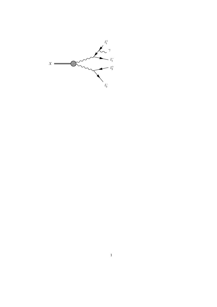
Figure 4: Radiative Diagram 1.

Figure 5: Radiative Diagram 2.

If the cutoff is small enough, the lepton momenta can be held fixed while the photon momentum is integrated out, with the result

$$\delta_{\text{brem}}=4\pi\alpha\int_{0}^{E_{\text{cut}}}\frac{d^{3}k}{(2\pi)^{3}2E_{k}}\mathcal{B},$$ (32)

where

$$\mathcal{B} =\sum_{\epsilon}\left|\left(\frac{p_{2}^{\mu}}{p_{2}\cdot k}+\frac{p_{4}^{\mu}}{p_{4}\cdot k}-\frac{p_{1}^{\mu}}{p_{1}\cdot k}-\frac{p_{3}^{\mu}}{p_{3}\cdot k}\right)\epsilon_{\mu}\right|^{2},$$ (33)

$$\begin{split}=\frac{2p_{1}\cdot p_{2}}{(p_{1}\cdot k)(p_{2}\cdot k)}+\frac{2p_{3}\cdot p_{4}}{(p_{3}\cdot k)(p_{4}\cdot k)}+\frac{2p_{1}\cdot p_{4}}{(p_{1}\cdot k)(p_{4}\cdot k)}\\ +\frac{2p_{2}\cdot p_{3}}{(p_{2}\cdot k)(p_{3}\cdot k)}-\frac{2p_{2}\cdot p_{4}}{(p_{2}\cdot k)(p_{4}\cdot k)}-\frac{2p_{1}\cdot p_{3}}{(p_{1}\cdot k)(p_{3}\cdot k)}\\ -\frac{p_{1}^{2}}{(p_{1}\cdot k)^{2}}-\frac{p_{2}^{2}}{(p_{2}\cdot k)^{2}}-\frac{p_{3}^{2}}{(p_{3}\cdot k)^{2}}-\frac{p_{4}^{2}}{(p_{4}\cdot k)^{2}}.\end{split}$$

The correction can be expressed in terms of a sum of ten integrals which can be done in closed form

$$\delta_{\text{brem}}=4\pi\alpha[2I(p_{1},p_{2})+2I(p_{3},p_{4})+2I(p_{1},p_{4})\\ +2I(p_{2},p_{3})-2I(p_{2},p_{4})-2I(p_{1},p_{3})\\ -I(p_{1},p_{1})-I(p_{2},p_{2})-I(p_{3},p_{3})-I(p_{4},p_{4})],$$ (34)

where

$$I(k_{i},k_{j})=\int_{0}^{E_{\text{cut}}}\frac{d^{3}k}{(2\pi)^{3}2E_{k}}\frac{k_{i}\cdot k_{j}}{(k_{i}\cdot k)(k_{j}\cdot k)}.$$ (35)

Each integral yields both a finite part and an IR divergent part which goes as $\ln(2{E_{\text{cut}}}/\Lambda)$ where $\Lambda$ is the photon mass which will be taken to zero after the divergent terms are canceled against each other. The first two divergent terms will be seen to cancel the divergent parts of the vertex correction, the next four cancel divergences in the 5–point functions, and the last four cancel the electron self–energy divergences (which are included in the renormalized vertex function). For $k_{i}\neq k_{j}$

$$I(k_{i}, k_{j})=\frac{z_{ij}}{8\pi^{2}\lambda_{ij}}\bigg{\{}\ln{\left(\frac{z_{ij}+\lambda_{ij}}{z_{ij}-\lambda_{ij}}\right)}\ln{\left(\frac{2{E_{\text{cut}}}}{\Lambda}\right)}$$

$$+\frac{1}{4}\ln^{2}{\bigg{(}\frac{\Omega_{i}^{-}}{\Omega_{i}^{+}}\bigg{)}}-\frac{1}{4}\ln^{2}{\bigg{(}\frac{\Omega_{j}^{-}}{\Omega_{j}^{+}}\bigg{)}}$$

$$+\operatorname{Li_{2}}{\left(1-\frac{\Upsilon_{ij}\Omega_{i}^{+}}{x_{ij}\lambda_{ij}}\right)}+\operatorname{Li_{2}}{\left(1-\frac{\Upsilon_{ij}\Omega_{i}^{-}}{x_{ij}\lambda_{ij}}\right)}$$

$$-\operatorname{Li_{2}}{\left(1-\frac{\Upsilon_{ij}\Omega_{j}^{+}}{x_{ij}\lambda_{ij}}\right)}-\operatorname{Li_{2}}{\left(1-\frac{\Upsilon_{ij}\Omega_{j}^{-}}{x_{ij}\lambda_{ij}}\right)}\bigg{\}},$$ (36)

where

$$\Omega_{i}^{\pm} =(1+\delta_{i,jkl}\pm\lambda_{i,jkl})/2,$$ (37a)

$$\Omega_{j}^{\pm} =(1+\delta_{j,ikl}\pm\lambda_{j,ikl})/(2\sigma_{ij}),$$ (37b)

$$\Upsilon_{ij} =\sigma_{ij}(1+\delta_{i,jkl})-(1+\delta_{j,ikl}),$$ (37c)

$$\sigma_{ij} =(z_{ij}+\lambda_{ij})/(1-z_{ij}+\delta_{ij}),$$ (37d)

and the various $\delta$, $z$, and $\lambda$ symbols are defined in Appendix A. For $k_{i}=k_{j}$

$$I(k_{i},k_{i})=\frac{1}{4\pi^{2}}\bigg{[}\ln{\left(\frac{2{E_{\text{cut}}}}{\Lambda}\right)}-\frac{1}{2\lambda_{ii}}\ln{\left(\frac{1+\lambda_{ii}}{1-\lambda_{ii}}\right)}\bigg{]},$$ (38)

where $\lambda_{ii}$ is again defined in Appendix A.

It will be enlightening to extract the IR divergent part of the soft brem contribution and express it in a way that will make the cancellation obvious. Collecting terms, one has

$$\delta_{\text{brem}}^{IR}=\ln\Lambda\bigg{\{}\frac{2\alpha}{\pi}\left[1-\frac{z_{12}}{2\lambda_{12}}\ln{\left(\frac{z_{12}+\lambda_{12}}{z_{12}-\lambda_{12}}\right)}\right]\\ +\frac{2\alpha}{\pi}\left[1-\frac{z_{34}}{2\lambda_{34}}\ln{\left(\frac{z_{34}+\lambda_{34}}{z_{34}-\lambda_{34}}\right)}\right]\\ +\frac{\alpha}{\pi}\frac{z_{13}}{\lambda_{13}}\ln{\left(\frac{z_{13}+\lambda_{13}}{z_{13}-\lambda_{13}}\right)}-\frac{\alpha}{\pi}\frac{z_{14}}{\lambda_{14}}\ln{\left(\frac{z_{14}+\lambda_{14}}{z_{14}-\lambda_{14}}\right)}\\ -\frac{\alpha}{\pi}\frac{z_{23}}{\lambda_{23}}\ln{\left(\frac{z_{23}+\lambda_{23}}{z_{23}-\lambda_{23}}\right)}+\frac{\alpha}{\pi}\frac{z_{24}}{\lambda_{24}}\ln{\left(\frac{z_{24}+\lambda_{24}}{z_{24}-\lambda_{24}}\right)}\bigg{\}}.$$ (39)

As will be seen shortly, the first two terms cancel the divergent part of the vertex correction while the last four cancel the divergent part of the 5–point correction.

V.2 Virtual Correction

As mentioned above, the virtual correction arises from the interference between the tree–level and one–loop diagrams. If the full matrix element is

$$\mathcal{M}=\mathcal{M}_{\text{tree}}+\mathcal{M}_{\text{virt}}+\mathcal{O}(e^{6}),$$ (40)

then the squared matrix element to $\mathcal{O}(\alpha^{3})$ is

$$|\mathcal{M}_{\text{rad}}|^{2} =|\mathcal{M}_{\text{tree}}|^{2}\left[1+\frac{2\operatorname{Re}{(\mathcal{M}_{\text{tree}}^{*}\mathcal{M}_{\text{virt}})}}{|\mathcal{M}_{\text{tree}}|^{2}}\right],$$ (41)

$$=|\mathcal{M}_{\text{tree}}|^{2}(1+\delta_{\text{virt}}).$$ (42)

This defines $\delta_{\text{virt}}$,

$$\delta_{\text{virt}}=\frac{2\operatorname{Re}{(\mathcal{M}_{\text{tree}}^{*}\mathcal{M}_{\text{virt}})}}{|\mathcal{M}_{\text{tree}}|^{2}}.$$ (43)

Therefore, we must compute the matrix element for each of the one–loop contributions.

V.2.1 Vacuum Polarization

The vacuum polarization process involves higher order corrections to the photon propagator and is a function of the square of the photon momentum, or the $x$ of that pair. There is one contribution for each photon propagator. One contribution is shown in Fig. 6.

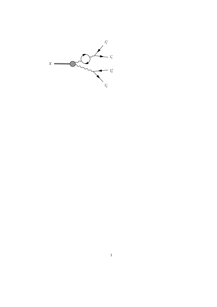
Figure 6: Vacuum Polarization Diagram.

The vacuum polarization diagram is IR finite but UV divergent. The divergence can be handled by renormalization of the photon wavefunction. The vacuum polarization matrix element can be written as the tree–level matrix element times the renormalized polarization insertion

$$\mathcal{M}_{\text{vp}}=\mathcal{M}_{\text{tree}}\sum_{l}\Pi_{l}(x_{ij}),$$ (44)

where the sum is over lepton species in the loop and the renormalized polarization insertion is

$$\Pi_{l}(x_{ij})=\frac{2\alpha}{\pi}\int_{0}^{1}dz\ z(1-z)\\ \times\ln\left[1-z(1-z)x_{ij}M^{2}/m_{l}^{2}-i\epsilon\right],$$ (45)

where $m_{l}$ is the mass of the lepton in the loop. The integration depends on the size of $x_{ij}$ compared to $m_{l}^{2}/M^{2}$, such that

$$\Pi_{l}(x_{ij})=-\frac{\alpha}{3\pi}\bigg{\{}\frac{8}{3}-\beta_{ij}^{2}\\ +\frac{\beta_{ij}}{2}(3-\beta_{ij}^{2})\left[\ln\left(\frac{1-\beta_{ij}}{1+\beta_{ij}}\right)+i\pi\right]\bigg{\}},$$ (46)

for $x_{ij}>4m_{l}^{2}/M^{2}$, while

$$\Pi_{l}(x_{ij})=-\frac{\alpha}{3\pi}\bigg{\{}\frac{8}{3}+\rho_{ij}^{2}\\ -\frac{\rho_{ij}}{2}(3+\rho_{ij}^{2})\left[\pi-2\tan^{-1}\rho_{ij}\right]\bigg{\}},$$ (47)

for $x_{ij}<4m_{l}^{2}/M^{2}$. The functions $\rho$ and $\beta$ are related to $\lambda$ as defined in Appendix A but are functions of the loop mass

$$\beta_{ij} =\sqrt{1-4m_{l}^{2}/(x_{ij}M^{2})},$$ (48a)

$$\rho_{ij} =\sqrt{4m_{l}^{2}/(x_{ij}M^{2})-1}.$$ (48b)

The correction then is

$$\delta_{\text{vp}}=2\sum_{g}\left[\sum_{l_{g}}\operatorname{Re}{\Pi_{l_{g}}(x_{ij})}\right],$$ (49)

where the first sum is over the number of vacuum polarization graphs and the second sum is over the possible lepton species in the loop.

V.2.2 Vertex Function

The vertex function involves higher order corrections to the QED vertex and is a function of the momenta of the pair. One contribution is shown in Fig. 7.

Figure 7: Vertex Correction Diagram.

Figure 8: 5–Point Diagram.

The vertex correction contains both UV and IR divergences. We will also include the self–energy correction to the lepton lines which also are UV and IR divergent. Both UV divergences will be handled simultaneously by renormalization of the electromagnetic coupling and the lepton wavefunction while the IR divergent part will cancel the IR divergence in the soft bremsstrahlung correction. The matrix element corresponding to one of the diagrams is

$$\mathcal{M}_{\text{vc}}=\mathcal{M}_{\text{tree}}\mathcal{V}(x_{ij},y_{ij}),$$ (50)

where

$$\mathcal{V}(x_{ij},y_{ij})=F_{1}(x_{ij})+F_{2}(x_{ij})\left[\frac{2}{2-\lambda_{ij}^{2}+y_{ij}^{2}}\right].$$ (51)

$F_{1}$ and $F_{2}$ are vertex form factors defined by

$$F_{1}( x_{ij})=\frac{\alpha}{\pi}\Bigg{(}\left\{1-\frac{z_{ij}}{2\lambda_{ij}}\left[\ln{\left(\frac{z_{ij}+\lambda_{ij}}{z_{ij}-\lambda_{ij}}\right)}-2i\pi\right]\right\}\ln\frac{m_{i}}{\Lambda}$$

$$-1+\frac{1+2\lambda_{ij}^{2}}{8\lambda_{ij}}\left[\ln{\left(\frac{z_{ij}+\lambda_{ij}}{z_{ij}-\lambda_{ij}}\right)}-2i\pi\right]$$

$$-\frac{z_{ij}}{\lambda_{ij}}\left[\operatorname{Li_{2}}\left(\frac{2\lambda_{ij}}{1+\lambda_{ij}}\right)+\frac{1}{16}\ln^{2}{\left(\frac{z_{ij}+\lambda_{ij}}{z_{ij}-\lambda_{ij}}\right)}-\frac{\pi^{2}}{2}\right]$$

$$+\frac{i\pi}{2}\frac{z_{ij}}{\lambda_{ij}}\ln\left(\frac{2\lambda_{ij}^{2}}{1-z_{ij}}\right)\Bigg{)},$$ (52)

$$F_{2}( x_{ij})=-\frac{\alpha}{\pi}\frac{1-z_{ij}}{4\lambda_{ij}}\left[\ln{\left(\frac{z_{ij}+\lambda_{ij}}{z_{ij}-\lambda_{ij}}\right)}-2i\pi\right],$$ (53)

where $z_{ij}$ and $\lambda_{ij}$ are defined in Appendix A and $\Lambda$ is the photon mass.

The correction is then just

$$\delta_{\text{vc}}=2\sum_{g}\operatorname{Re}{\mathcal{V}(x_{ij},y_{ij})},$$ (54)

where the sum over $g$ is over the number of vertex function graphs.

The IR divergent part is contained within $F_{1}$. Twice the real part of the $\ln\Lambda$ term is exactly what is necessary to cancel the first two divergent terms (one for each vertex correction graph) in the soft brem contribution. The final four divergent soft brem terms will have to wait for the last piece of the virtual correction, the 5–point diagram.

V.2.3 5–Point Diagram

There are four distinct 5–point diagrams that contribute to the direct process, plus four more if there is an exchange process. The diagram shown in Fig. 8 contains a photon exchanged between $l^{-}_{1}$ and $l^{+}_{2}$. The matrix element for that graph is

$$\mathcal{M}_{\text{5p}}^{1}=\int\frac{d^{4}t}{(2\pi)^{4}}\frac{2}{M}\left[\mathcal{F}_{P}\epsilon_{\mu\nu\rho\sigma}+\mathcal{F}_{S}(g_{\mu\rho}g_{\nu\sigma}-g_{\mu\sigma}g_{\nu\rho})\right](p_{12}+t)^{\mu}(p_{34}-t)^{\rho}\\ \times\left[\frac{-ig^{\delta\eta}}{t^{2}-\lambda^{2}+i\epsilon}\right]\left[\frac{-ig^{\alpha\nu}}{(p_{12}+t)^{2}-\lambda^{2}+i\epsilon}\right]\left[\frac{-ig^{\beta\sigma}}{(p_{34}-t)^{2}-\lambda^{2}+i\epsilon}\right]\\ \times\bar{u}(p_{2})(-ie\gamma_{\delta})\left(\frac{i}{\hbox to0.0pt{/\hss}{t}+\hbox to0.0pt{/\hss}{p_{2}}-m_{1}+i\epsilon}\right)(-ie\gamma_{\alpha})v(p_{1})\bar{u}(p_{4})(-ie\gamma_{\beta})\left(\frac{i}{\hbox to0.0pt{/\hss}{t}-\hbox to0.0pt{/\hss}{p_{3}}-m_{2}+i\epsilon}\right)(-ie\gamma_{\eta})v(p_{3}),$$ (55)

where $t$ is the loop momentum and $p_{1}$, $p_{2}$, $p_{3}$, and $p_{4}$ are the momenta of $l^{+}_{1}$, $l^{-}_{1}$, $l^{+}_{2}$, and $l^{-}_{2}$, respectively. This can be re–expressed as

$$\mathcal{M}_{\text{5p}}^{1} =-\frac{2ie^{4}}{M}\bigg{(}\mathcal{F}_{P}\ \epsilon_{\mu\rho\nu\sigma}\big{\{}-p_{12}^{\mu}p_{34}^{\rho}\big{[}I_{50}A^{\nu\sigma}+I_{51}^{\alpha}B^{\nu\sigma}_{\ \ \alpha}+I_{52}^{\alpha\beta}C^{\nu\sigma}_{\ \ \alpha\beta}\big{]}+p_{5}^{\mu}\big{[}I_{51}^{\rho}A^{\nu\sigma}+I_{52}^{\rho\alpha}B^{\nu\sigma}_{\ \ \alpha}+I_{53}^{\rho\alpha\beta}C^{\nu\sigma}_{\ \ \alpha\beta}\big{]}\big{\}}$$

$$+\mathcal{F}_{S}\big{\{}[(p_{12}\cdot p_{34})g^{\mu\nu}-p_{5}^{\mu}p_{5}^{\nu}]\big{[}I_{50}A_{\mu\nu}+I_{51}^{\alpha}B_{\mu\nu\alpha}+I_{52}^{\alpha\beta}C_{\mu\nu\alpha\beta}\big{]}+(p_{34}-p_{12})_{\rho}g_{\mu\nu}\big{[}I_{51}^{\rho}A^{\mu\nu}+I_{52}^{\rho\alpha}B^{\mu\nu}_{\ \ \alpha}+I_{53}^{\rho\alpha\beta}C^{\mu\nu}_{\ \ \alpha\beta}\big{]}$$

$$\quad\quad\quad-g_{\mu\nu}\big{[}(I_{52})^{\rho}_{\rho}A^{\mu\nu}+(I_{53})^{\rho}_{\alpha\rho}B^{\alpha\mu\nu}+(I_{54})^{\rho}_{\alpha\beta\rho}C^{\alpha\beta\mu\nu}\big{]}\big{\}}\bigg{)},$$ (56)

where $A$, $B$, and $C$ are combinations of spinors and gamma matrices and $p_{5}=p_{1}+p_{2}+p_{3}+p_{4}$. The factors of $I_{i}$ are integrals over the loop momentum. There are three basic integral forms from which all the other may be obtained. The notation for the integrals has the following meaning: the first digit in the subscript refers to the number of denominators and the second refers the number of powers of the loop momentum appearing in the integral. The 5–point integrals are defined in Appendix D as a function of four 4–vector arguments $k_{1}$, $k_{2}$, $k_{3}$, $k_{4}$.

For the diagram shown in Fig. 8, the arguments of the 5–point integral functions should take on the values

$$k_{1} =-p_{2}, k_{2} =-p_{1},$$ (57a)

$$k_{3} =p_{5}, k_{4} =-p_{4},$$ (57b)

so we can write

$$I_{50}=I_{50}(-p_{2},-p_{1},p_{5},-p_{4})$$ (58)

for the scalar integral, and analogous expressions for the higher-rank tensor integrals. The spinor terms for this diagram are

$$A^{\mu\nu} =-4(p_{2}\cdot p_{3})\bar{u}(p_{2})\gamma^{\mu}v(p_{1})\bar{u}(p_{4})\gamma^{\nu}v(p_{3}),$$ (59a)

$$B^{\mu\nu\rho} =2[\bar{u}(p_{2})\gamma^{\nu}v(p_{1})\bar{u}(p_{4})\gamma^{\rho}\gamma^{\mu}\hbox to0.0pt{/\hss}p_{2}v(p_{3})$$

$$\quad-\bar{u}(p_{2})\hbox to0.0pt{/\hss}p_{3}\gamma^{\mu}\gamma^{\nu}v(p_{1})\bar{u}(p_{4})\gamma^{\rho}v(p_{3})],$$ (59b)

$$C^{\mu\nu\rho\sigma} =\bar{u}(p_{2})\gamma^{\eta}\gamma^{\mu}\gamma^{\rho}v(p_{1})\bar{u}(p_{4})\gamma^{\sigma}\gamma^{\nu}\gamma_{\eta}v(p_{3}).$$ (59c)

The spinor terms for the diagram containing a photon exchanged between $l^{-}_{1}$ and $l^{-}_{2}$ are

$$A^{\mu\nu} =4(p_{2}\cdot p_{4})\bar{u}(p_{2})\gamma^{\mu}v(p_{1})\bar{u}(p_{4})\gamma^{\nu}v(p_{3}),$$ (60a)

$$B^{\mu\nu\rho} =2[\bar{u}(p_{2})\hbox to0.0pt{/\hss}p_{4}\gamma^{\mu}\gamma^{\nu}v(p_{1})\bar{u}(p_{4})\gamma^{\rho}v(p_{3})$$

$$\quad-\bar{u}(p_{2})\gamma^{\nu}v(p_{1})\bar{u}(p_{4})\hbox to0.0pt{/\hss}p_{2}\gamma^{\mu}\gamma^{\rho}v(p_{3})],$$ (60b)

$$C^{\mu\nu\rho\sigma} =-\bar{u}(p_{2})\gamma^{\eta}\gamma^{\mu}\gamma^{\rho}v(p_{1})\bar{u}(p_{4})\gamma_{\eta}\gamma^{\nu}\gamma^{\sigma}v(p_{3}),$$ (60c)

and the scalar integral for this diagram is

$$I_{50}=I_{50}(-p_{2},-p_{1},p_{5},-p_{3}).$$ (61)

The spinor terms for the diagram containing a photon exchanged between $l^{+}_{1}$ and $l^{+}_{2}$ are

$$A^{\mu\nu} =4(p_{1}\cdot p_{3})\bar{u}(p_{2})\gamma^{\mu}v(p_{1})\bar{u}(p_{4})\gamma^{\nu}v(p_{3}),$$ (62a)

$$B^{\mu\nu\rho} =2[\bar{u}(p_{2})\gamma^{\nu}\gamma^{\mu}\hbox to0.0pt{/\hss}p_{3}v(p_{1})\bar{u}(p_{4})\gamma^{\rho}v(p_{3})$$

$$\quad-\bar{u}(p_{2})\gamma^{\nu}v(p_{1})\bar{u}(p_{4})\gamma^{\rho}\gamma^{\mu}\hbox to0.0pt{/\hss}p_{1}v(p_{3})],$$ (62b)

$$C^{\mu\nu\rho\sigma} =-\bar{u}(p_{2})\gamma^{\rho}\gamma^{\mu}\gamma^{\eta}v(p_{1})\bar{u}(p_{4})\gamma^{\sigma}\gamma^{\nu}\gamma_{\eta}v(p_{3}),$$ (62c)

and the scalar integral for this diagram is

$$I_{50}=I_{50}(-p_{1},-p_{2},p_{5},-p_{4}).$$ (63)

The spinor terms for the diagram containing a photon exchanged between $l^{+}_{1}$ and $l^{-}_{2}$ are

$$A^{\mu\nu} =-4(p_{1}\cdot p_{4})\bar{u}(p_{2})\gamma^{\mu}v(p_{1})\bar{u}(p_{4})\gamma^{\nu}v(p_{3}),$$ (64a)

$$B^{\mu\nu\rho} =2[\bar{u}(p_{2})\gamma^{\nu}v(p_{1})\bar{u}(p_{4})\hbox to0.0pt{/\hss}p_{1}\gamma^{\mu}\gamma^{\rho}v(p_{3})$$

$$\quad-\bar{u}(p_{2})\gamma^{\nu}\gamma^{\mu}\hbox to0.0pt{/\hss}p_{4}v(p_{1})\bar{u}(p_{4})\gamma^{\rho}v(p_{3})],$$ (64b)

$$C^{\mu\nu\rho\sigma} =\bar{u}(p_{2})\gamma^{\rho}\gamma^{\mu}\gamma^{\eta}v(p_{1})\bar{u}(p_{4})\gamma_{\eta}\gamma^{\nu}\gamma^{\sigma}v(p_{3}),$$ (64c)

and the scalar integral for this diagram is

$$I_{50}=I_{50}(-p_{1},-p_{2},p_{5},-p_{3}).$$ (65)

The tensors $A$, $B$, and $C$ are computed for a given helicity combination and combined with the integrals to yield the matrix element for that helicity state. The correction then involves a sum over the sixteen possible final states

$$\delta_{\text{5p}}=\frac{\sum_{\lambda=1}^{16}2\operatorname{Re}{\left[\mathcal{M}_{\text{tree}}^{*}(\lambda)\mathcal{M}_{\text{5p}}(\lambda)\right]}}{\sum_{\lambda=1}^{16}\left|\mathcal{M}_{\text{tree}}(\lambda)\right|^{2}},$$ (66)

where $\lambda$ here refers to the helicity state and

$$\mathcal{M}_{\text{tree}}(\lambda) =\sum_{g}\mathcal{M}_{\text{tree}}^{g}(\lambda),$$ (67)

$$\mathcal{M}_{\text{5p}}(\lambda) =\sum_{g}\mathcal{M}_{\text{5p}}^{g}(\lambda).$$ (68)

The sums here are over the number of graphs for each process.

The IR divergent part of the 5–point correction is most easily isolated by looking at the 5–point matrix element in the IR limit. All terms involving tensor integrals vanish leaving only the $I_{50}$ term. The divergent part of $I_{50}$ is due to the two divergent box integrals, $I_{40}^{(3)}$ and $I_{40}^{(4)}$. The relevant terms in the scalar 5–point function for Fig. 8, in terms of the divergent 3–point function, are

$$I_{50}^{IR} =-\frac{1}{2}\left(\frac{\sum_{j}S_{3j}^{-1}}{p_{34}^{2}-M_{2}^{2}}+\frac{\sum_{j}S_{4j}^{-1}}{p_{12}^{2}-M_{1}^{2}}\right)I_{IR},$$

$$=I_{IR}/\left[(p_{12}^{2}-M_{1}^{2})(p_{34}^{2}-M_{2}^{2})\right].$$ (69)

Extracting the $\ln\Lambda$ piece of $I_{IR}$, $I_{50}^{IR}$ can be written as

$$I_{50}^{IR}=\frac{-i}{16\pi^{2}\lambda_{23}p_{23}^{2}(p_{12}^{2}-M_{1}^{2})(p_{34}^{2}-M_{2}^{2})}\\ \times\left[\ln{\left(\frac{z_{23}+\lambda_{23}}{z_{23}-\lambda_{23}}\right)}-2i\pi\right]\ln\frac{\Lambda}{\mu},$$ (70)

where $\mu$ is a kinematic function with dimensions of mass which is independent of $\Lambda$. The divergent part of the 5–point matrix element, dropping the finite term involving $\mu$, is proportional to the tree–level matrix element

$$\mathcal{M}_{\text{5p}}^{IR}=\mathcal{M}_{\text{tree}}\frac{\alpha}{2\pi}\frac{z_{23}}{\lambda_{23}}\left[\ln{\left(\frac{z_{23}+\lambda_{23}}{z_{23}-\lambda_{23}}\right)}-2i\pi\right]\ln\Lambda.$$ (71)

The IR divergent part of the 5–point correction coming from all four diagrams is

$$\delta_{\text{5p}}^{IR}=\sum_{g}-s_{ij}\frac{\alpha}{\pi}\frac{z_{ij}}{\lambda_{ij}}\ln{\left(\frac{z_{ij}+\lambda_{ij}}{z_{ij}-\lambda_{ij}}\right)}\ln\Lambda,$$ (72)

where $s_{ij}$ is the product of the sign of the charges of $p_{i}$ and $p_{j}$ and the sum is over the four diagrams. Again, it can be seen that this is the necessary form to cancel the remaining four divergent brem terms.

VI MC Simulation Results

The inclusion of the radiative corrections impacts both the differential rate and the total rate. The total correction to the differential $\pi^{0}\to e^{+}e^{-}e^{+}e^{-}$ rate is shown in Fig. 9.

Figure 9: Distribution of the total radiative correction for $\pi^{0}\to eeee$ events with an IR cutoff of $x_{4e}^{\text{cut}}=0.9985$, with $f_{P}=f_{S}=1$.

The average size of the correction factor for the four different modes is shown in Table 5.

Table 5: Average size of radiative correction to the differential rate with an IR cutoff of $x_{4e}^{\text{cut}}=0.9985$, with $f_{P}=f_{S}=1$.

	$\pi^{0}\to eeee$	$K_{L}\to eeee$	$K_{L}\to ee\mu\mu$	$K_{L}\to\mu\mu\mu\mu$
$\bar{\delta}$	$-0.1948$	$-0.2618$	$-0.0788$	$+0.0805$

The total rate for the combined 4–lepton plus photon process is independent of IR cutoff. Table 6 summarizes the tree–level rate and the rate for the combined, cutoff independent process, divided into the rate including all radiation and the rate including only soft radiation ($x_{4e}>0.95$), all with $f_{P}=f_{S}=1$.

Table 6: Summary of tree–level 4–lepton rate and combined radiatively corrected 4–lepton plus photon rate, including the rate for all $x_{4e}$ and the rate for $x_{4e}>0.95$, using $f_{P}=f_{S}=1$.

		$\Gamma_{4l(\gamma)}/\Gamma_{\gamma\gamma}$
Mode	$\Gamma_{4l}^{tree}/\Gamma_{\gamma\gamma}$	all $x_{4e}$	$x_{4e}>0.95$
$\pi^{0}\to eeee$	$3.421(4)\cdot 10^{-5}$	$3.536(4)\cdot 10^{-5}$	$3.331(4)\cdot 10^{-5}$
$K_{L}\to eeee$	$6.222(5)\cdot 10^{-5}$	$6.406(4)\cdot 10^{-5}$	$5.903(4)\cdot 10^{-5}$
$K_{L}\to ee\mu\mu$	$2.858(1)\cdot 10^{-6}$	$2.996(3)\cdot 10^{-6}$	$2.909(3)\cdot 10^{-6}$
$K_{L}\to\mu\mu\mu\mu$	$0.941(1)\cdot 10^{-9}$	$1.026(1)\cdot 10^{-9}$	$1.025(1)\cdot 10^{-9}$

It is the last column which should most accurately predict the observed non–radiative 4–lepton rate. It is seen that the non–radiative rate is smaller than the tree–level rate for both 4–electron modes while it is larger for the modes with muons.

The probability of radiation can now be computed as the ratio of the radiative rate to the combined rate. Table 7 lists the probability of radiating a photon ($x_{4e}<0.9985$) along with the probability of radiating a hard photon ($x_{4e}<0.95$) for each of the four modes.

Table 7: Probability of radiation ($x_{4e}<0.9985$) and probability of hard radiation ($x_{4e}<0.95$), defined as $P=\Gamma_{4l\gamma}/\Gamma_{4l(\gamma)}$.

Mode	$P(x_{4e}<0.9985)$	$P(x_{4e}<0.95)$
$\pi^{0}\to eeee(\gamma)$	0.187	0.058
$K_{L}\to eeee(\gamma)$	0.240	0.079
$K_{L}\to ee\mu\mu(\gamma)$	0.109	0.029
$K_{L}\to\mu\mu\mu\mu(\gamma)$	0.006	0.0003

The probability is highest for $K_{L}\to e^{+}e^{-}e^{+}e^{-}(\gamma)$ where the $x$ values can be the smallest. The probabilities for $K_{L}\to e^{+}e^{-}\mu^{+}\mu^{-}(\gamma)$ are slightly less than half of what they are for the four electron mode, and in $K_{L}\to\mu^{+}\mu^{-}\mu^{+}\mu^{-}(\gamma)$, there is very little radiation.

The effect of the radiative corrections on the differential rate can be observed in the distributions of the five phase space variables. The statistics in the following plots reflect the amount of CPU time dedicated to each mode. While the calculation of the radiative corrections is CPU–intensive, it is actually the generation of the radiative decays that takes the most time.

For the modes with identical leptons, it is useful to adopt a method of pairing the electrons with the positrons in order to study the dilepton mass distributions. We choose to use the pairing for which the product of $x$’s is minimized. It is this pairing that will contribute the most to the matrix element in general. Therefore, $x_{a}$ and $x_{b}$ are the $x$’s belonging to this pairing, with the additional requirement that $x_{a}<x_{b}$. In addition, $y_{a}$ is the $y$ variable defined in the $a$–pair CM, and $y_{b}$ is the same quantity in the $b$–pair CM. And lastly, $\phi_{ab}$ is the angle between the planes of the $a$–pair and $b$–pair in the overall CM.

The first variable that we will look at is $x$ which is modified by both the existence of a form factor and the inclusion of the radiative corrections. In all cases we set $\beta=0$ in the DIP form factor model. Figs. 10 and 11 show the distribution of $x_{a}$ and $x_{b}$, respectively, for $\pi^{0}\to e^{+}e^{-}e^{+}e^{-}$ events. The plot on the left compares the distribution using the tree–level matrix element with no form factor ($\alpha=0$) to that using the same matrix element but with $\alpha=-1.0$. The plot on the right compares the distribution using the tree–level matrix element with no form factor to that using the radiatively–corrected matrix element also with no form factor.

Figure 10: (a) $x_{a}$ in $\pi^{0}\to eeee$ events using the tree–level differential rate with $\alpha=0$ (dots) and with $\alpha=-1.0$ (histogram). (b) $x_{a}$ in $\pi^{0}\to eeee$ events using the tree–level differential rate with $\alpha=0$ (dots) and the corrected rate for events with $x_{4e}>0.95$, also with $\alpha=0$ (histogram). The ratio of the dots to the histogram in both cases are shown in (c) and (d).

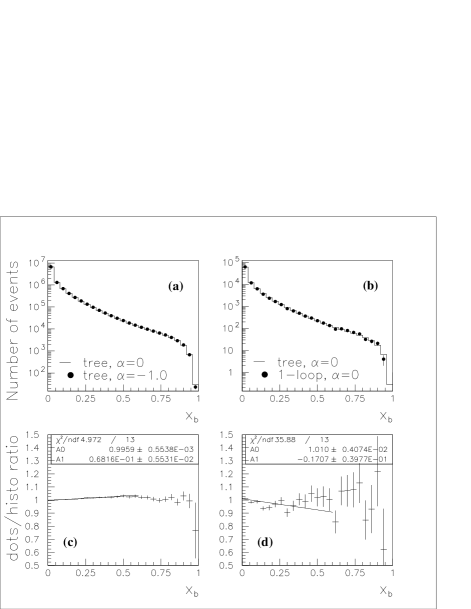
Figure 11: (a) $x_{b}$ in $\pi^{0}\to eeee$ events using the tree–level differential rate with $\alpha=0$ (dots) and with $\alpha=-1.0$ (histogram). (b) $x_{b}$ in $\pi^{0}\to eeee$ events using the tree–level differential rate with $\alpha=0$ (dots) and the corrected rate for events with $x_{4e}>0.95$, also with $\alpha=0$ (histogram). The ratio of the dots to the histogram in both cases are shown in (c) and (d).

We have provided a linear fit to the ratio over some reasonable range on a scale appropriate for comparing the two effects. For the form factor comparisons, the dependence should be primarily linear. This is not the case for the radiative corrections in general. The $\chi^{2}$ per degree of freedom is included as a measure of the linearity. It can be seen that the form factor has a much smaller effect on the $x$ distribution than the radiative corrections do. This is not too surprising since the range of accessible $q^{2}$ values for the $\pi^{0}$ decay is relatively small in addition to being far from our assumed $\rho$ pole.

For the kaon modes, we observe that the form factor has a much larger effect on the $x$ distribution than the radiative corrections do. Figs. 12 and 13 show the distribution of $x_{a}$ and $x_{b}$, respectively, for $K_{L}\to e^{+}e^{-}e^{+}e^{-}$ events. The plot on the left compares the distribution using the tree–level matrix element with no form factor ($\alpha=0$) to that using the same matrix element but with $\alpha=-1.5$. The plot on the right compares the distribution using the tree–level matrix element with no form factor to that using the radiatively–corrected matrix element also with no form factor.

Figure 12: (a) $x_{a}$ in $K_{L}\to eeee$ events using the tree–level differential rate with $\alpha=0$ (dots) and with $\alpha=-1.5$ (histogram). (b) $x_{a}$ in $K_{L}\to eeee$ events using the tree–level differential rate with $\alpha=0$ (dots) and the corrected rate for events with $x_{4e}>0.95$, also with $\alpha=0$ (histogram). The ratio of the dots to the histogram in both cases are shown in (c) and (d).

Figure 13: (a) $x_{b}$ in $K_{L}\to eeee$ events using the tree–level differential rate with $\alpha=0$ (dots) and with $\alpha=-1.5$ (histogram). (b) $x_{b}$ in $K_{L}\to eeee$ events using the tree–level differential rate with $\alpha=0$ (dots) and the corrected rate for events with $x_{4e}>0.95$, also with $\alpha=0$ (histogram). The ratio of the dots to the histogram in both cases are shown in (c) and (d).

The roll off at high $x$ in plot (c) of Fig. 13 is due to presence of the exchange diagram in this mode. Figs. 14 and 15 show the same distributions for $K_{L}\to e^{+}e^{-}\mu^{+}\mu^{-}$ events. Here there are no pairing ambiguities and we plot $x_{ee}$ and $x_{\mu\mu}$.

Figure 14: (a) $x_{ee}$ in $K_{L}\to ee\mu\mu$ events using the tree–level differential rate with $\alpha=0$ (dots) and with $\alpha=-1.5$ (histogram). (b) $x_{ee}$ in $K_{L}\to ee\mu\mu$ events using the tree–level differential rate with $\alpha=0$ (dots) and the corrected rate for events with $x_{4e}>0.95$, also with $\alpha=0$ (histogram). The ratio of the dots to the histogram in both cases are shown in (c) and (d).

Figure 15: (a) $x_{\mu\mu}$ in $K_{L}\to ee\mu\mu$ events using the tree–level differential rate with $\alpha=0$ (dots) and with $\alpha=-1.5$ (histogram). (b) $x_{\mu\mu}$ in $K_{L}\to ee\mu\mu$ events using the tree–level differential rate with $\alpha=0$ (dots) and the corrected rate for events with $x_{4e}>0.95$, also with $\alpha=0$ (histogram). The ratio of the dots to the histogram in both cases are shown in (c) and (d).

It can be seen that there is no roll off in plot (c) of Fig. 15, and furthermore, a small quadratic dependence is observable. While the $x$ of the $ee$ pair is slightly modified by the radiative corrections, the $x$ of the $\mu\mu$ pair does not change at all. This is as expected for the massive muons.

Fig. 16 shows the distribution of $y_{a}$ and $y_{b}$ for the tree level differential rate and the radiatively corrected differential rate for $K_{L}\to e^{+}e^{-}e^{+}e^{-}$ events.

Figure 16: (a) $y_{a}$ in $K_{L}\to eeee$ events using the tree–level differential rate (dots) and the corrected rate for events with $x_{4e}>0.95$ (histogram). (b) $y_{b}$ for the same events. The ratio of the corrected distributions to the tree–level distributions are shown in (c) and (d).

The effect here is quite small. Since $y$ is a measure of the energy asymmetry of the lepton pair, it is seen that the radiative corrections tend to make the pairs slightly more asymmetric on average.

The effect on the $\phi$ distribution is due entirely to the 5–point diagram. Fig. 17 shows a comparison of the distribution of $\phi_{ab}$ generated with the tree–level matrix element to the same distribution generated with the radiative corrections, for $K_{L}\to\mu^{+}\mu^{-}\mu^{+}\mu^{-}$ events.

Figure 17: (a) The distribution of $\phi_{ab}$ in $K_{L}\to\mu\mu\mu\mu$ events using the tree–level differential rate (dots) and the corrected rate for events with $x_{4e}>0.95$(histogram). (b) The ratio of the corrected distribution to the tree–level distribution.

The enhancement at $\phi_{ab}=\pi$ and the corresponding depletion at $\phi_{ab}=0=2\pi$ can be understood in terms of Coulomb interaction between the final state particles. The configuration at $\phi=0$ has all leptons in a plane with the same sign particles near each other. The effect is only observable in the $K_{L}\to\mu^{+}\mu^{-}\mu^{+}\mu^{-}$ decay where the leptons in each pair are usually well separated.

VII Conclusions

The main conclusion that can be drawn from these distributions is that the radiative corrections are extremely important for extracting a form factor in the $\pi^{0}\to e^{+}e^{-}e^{+}e^{-}$ mode. For the kaon modes, the form factor has a larger impact on the $x$ distribution and the modification of the distribution due to the radiative corrections is less important. The only published result for the $K_{L}\to e^{+}e^{-}e^{+}e^{-}$ mode Alavi-Harati et al. (2001a) quotes $\alpha_{DIP}=-1.1\pm 0.6(\text{stat})$. Fig. 13 shows that at most the radiative corrections would change the slope by $0.22$, which while significant, is smaller than the current experimental error. Likewise, for the $K_{L}\to e^{+}e^{-}\mu^{+}\mu^{-}$ mode, the latest resultHamm (2002) based on the invariant mass shape is $\alpha_{DIP}=-4.53^{+1.81}_{-2.70}$. The present experimental error is again larger than the impact of the radiative corrections on the mass distribution.

As for the extraction of the mixing angle $\zeta$ from the observed $\phi$ distribution, the radiative corrections can be safely neglected at present.

The two publications above quote an integrated rate (normalized to the two–photon rate) of $(6.24\pm 0.34)\cdot 10^{-5}$ for $K_{L}\to e^{+}e^{-}e^{+}e^{-}$ and $(4.51\pm 0.42)\cdot 10^{-6}$ for $K_{L}\to e^{+}e^{-}\mu^{+}\mu^{-}$, where the errors are purely statistical. These results are in good agreement with our predictions when both the radiative corrections and a form factor with $\alpha=-1.5$ are included. For $K_{L}\to e^{+}e^{-}e^{+}e^{-}$, the two effects offset and the net result is an increase of just less than $2\%$ over the tree–level rate with no form factor. In $K_{L}\to e^{+}e^{-}\mu^{+}\mu^{-}$, the form factor is the dominant effect.

Appendix A Kinematics

The four particle final state can be kinematically described by considering subsystems containing only two particles. Consider the system composed of two particles with momenta $p_{i}$ and $p_{j}$ and total momentum $p_{ij}=p_{i}+p_{j}$ and mass squared $m_{ij}^{2}=p_{ij}^{2}$. We will define a dimensionless dot product of any two vectors $p_{i}$ and $p_{j}$ as

$$z_{ij}=2(p_{i}\cdot p_{j})/p_{ij}^{2}=1-x_{i}-x_{j},$$ (73)

where

$$x_{i}=p_{i}^{2}/p_{ij}^{2},\quad x_{j}=p_{j}^{2}/p_{ij}^{2}.$$ (74)

The energy and momentum of each particle in the two–particle CM frame are

$$E_{i}^{*}=m_{ij}(1+\delta_{ij})/2,\quad E_{j}^{*}=m_{ij}(1-\delta_{ij})/2,$$ (75)

$$p^{*}=m_{ij}\lambda_{ij}/2,$$ (76)

where

$$\delta_{ij} =x_{i}-x_{j},$$ (77)

$$\lambda_{ij} =\sqrt{z_{ij}^{2}-w_{ij}^{2}},$$ (78)

$$w_{ij} =2\sqrt{x_{i}x_{j}}.$$ (79)

Occasionally we will use symbols like $z_{i,jk}$ whose meaning is interpreted as $z(p_{i},p_{j}+p_{k})$.

Now consider a three body system composed of momenta $p_{i}$, $p_{j}$, and $p_{k}$. There are two phase space variables needed to describe the system. The first one will be $x_{ij}=p_{ij}^{2}/p_{ijk}^{2}$. The other one is defined in the $ij$ CM frame as the cosine of the angle between the direction of particle $i$ and particle $k$,

$$\cos{\theta_{ij,k}}=\frac{2p_{k}\cdot(p_{i}-p_{j})-p_{ijk}^{2}\delta_{ij}z_{ij,k}}{p_{ijk}^{2}\lambda_{ij}\lambda_{ij,k}},$$ (80)

A more convenient variable that will be used in place of $\cos{\theta_{ij,k}}$ is

$$y_{ij}=\lambda_{ij}\cos{\theta_{ij,k}},$$ (81)

where $k$ will always refer to the total momentum minus the $ij$ momentum.

Finally, the four body final state requires five phase space variables to uniquely describe it. We will use the $x$ and $y$ values for the two lepton pairs plus the angle between the normals of the planes defined by each pair in the overall CM frame. The first four variables are

$$x_{12} =p_{12}^{2}/M^{2},$$ (82)

$$x_{34} =p_{34}^{2}/M^{2},$$ (83)

$$y_{12} =\frac{2p_{34}\cdot(p_{1}-p_{2})}{M^{2}\lambda},$$ (84)

$$y_{34} =\frac{2p_{12}\cdot(p_{3}-p_{4})}{M^{2}\lambda},$$ (85)

where the second term in the numerator of the $y$’s vanishes since $\delta_{12}=\delta_{34}=0$. Any use of $z$, $w$, or $\lambda$ without subscripts will refer to the functions of $x_{12}$ and $x_{34}$, so $\lambda=\lambda_{12,34}$ for instance. The last phase space variable is defined as

$$\phi=\tan^{-1}{(\sin{\phi}/\cos{\phi})},$$ (86)

where

$$\sin{\phi} =\frac{16\epsilon_{\mu\nu\rho\sigma}p_{1}^{\mu}p_{2}^{\nu}p_{3}^{\rho}p_{4}^{\sigma}}{M^{4}\lambda w\sqrt{(\lambda_{12}^{2}-y_{12}^{2})(\lambda_{34}^{2}-y_{34}^{2})}},$$ (87)

$$\cos{\phi} =\frac{M^{2}zy_{12}y_{34}-2(p_{1}-p_{2})\cdot(p_{3}-p_{4})}{M^{2}w\sqrt{(\lambda_{12}^{2}-y_{12}^{2})(\lambda_{34}^{2}-y_{34}^{2})}}.$$ (88)

The angle $\phi$ is defined so that at $\phi=0$ the two pairs lie in a plane with the like–sign particles adjacent to each other. The orientation of $\phi=\pi$ again has both pairs in a plane, but with the opposite signed particles adjacent.

The general expression for the phase space integral is

$$d^{8}\Phi=\frac{1}{(2\pi)^{8}}\frac{d^{3}p_{1}d^{3}p_{2}d^{3}p_{3}d^{3}p_{4}}{16E_{p_{1}}E_{p_{2}}E_{p_{3}}E_{p_{4}}}\delta^{4}(P-p_{1}-p_{2}-p_{3}-p_{4}).$$ (89)

Upon integrating out the $\delta$–functions, integrating over the Euler angles, and changing variables to those listed above, the phase space reduces to

$$d^{5}\Phi=\mathcal{S}\frac{M^{4}}{2^{14}\pi^{6}}\lambda dx_{12}dx_{34}dy_{12}dy_{34}d\phi,$$ (90)

where the factor $\mathcal{S}$ is a symmetry factor which is required for modes containing identical particles in the final state. The double Dalitz modes with identical particles contain two sets, thus requiring two factors of $1/2$. So $\mathcal{S}=1/4$ if the final state contains identical particles, and $\mathcal{S}=1$ otherwise.

When there are identical leptons in the final state, the amplitudes for the exchange diagrams have the same algebraic form as for the non–exchange diagrams except that the kinematic variables $x_{12}$, $x_{34}$, $y_{12}$, $y_{34}$, and $\phi$ are replaced by $x_{14}$, $x_{23}$, $y_{14}$, $y_{23}$, and $\phi_{14,23}$. These exchange variables will in general be functions of all five of the non–exchange variables. As is turns out, we only need explicit representations for $x_{14}$ and $x_{23}$. These are given by

$$x_{14} =[1-\lambda_{12}^{2}x_{12}-\lambda_{34}^{2}x_{34}-\lambda(y_{12}-y_{34})-zy_{12}y_{34}$$

$$\quad\quad+w\sqrt{(\lambda_{12}^{2}-y_{12}^{2})(\lambda_{34}^{2}-y_{34}^{2})}\cos{\phi}]/4,$$ (91)

$$x_{23} =[1-\lambda_{12}^{2}x_{12}-\lambda_{34}^{2}x_{34}+\lambda(y_{12}-y_{34})-zy_{12}y_{34}$$

$$\quad\quad+w\sqrt{(\lambda_{12}^{2}-y_{12}^{2})(\lambda_{34}^{2}-y_{34}^{2})}\cos{\phi}]/4.$$ (92)

Appendix B Meson–$\gamma\gamma$ Couplings

In this section we will work out the explicit form of the two–photon couplings, allowing for photons of arbitrary mass, using the polarization vectors in the helicity basis. The general form of the coupling is

$$\mathcal{H}_{\lambda_{1}\lambda_{2}}=H_{\mu\nu\rho\sigma}k_{1}^{\mu}\epsilon_{\lambda_{1}}^{*\nu}k_{2}^{\rho}\epsilon_{\lambda_{2}}^{*\sigma},$$ (93)

where $H$ is either

$$H_{\mu\nu\rho\sigma}^{P} =\frac{2}{M}\mathcal{F}_{P}\,\epsilon_{\mu\nu\rho\sigma},$$ (94a)

$$H_{\mu\nu\rho\sigma}^{S} =\frac{2}{M}\mathcal{F}_{S}(g_{\mu\rho}g_{\nu\sigma}-g_{\mu\sigma}g_{\nu\rho}).$$ (94b)

The three polarization vectors for a massive photon in the helicity basis are chosen to be

$$\epsilon^{+}(\pm\hat{\bm{z}}) =\left(0,1,\pm i,0\right)/\sqrt{2},$$ (95a)

$$\epsilon^{-}(\pm\hat{\bm{z}}) =\left(0,1,\mp i,0\right)/\sqrt{2},$$ (95b)

$$\epsilon^{0}(\pm\hat{\bm{z}}) =\left(k,0,0,\pm E\right)/\sqrt{k^{2}},$$ (95c)

for a photon traveling in the $\pm\hat{\bm{z}}$ direction. With these polarization vectors, one finds three couplings for the scalar case

$$\mathcal{H}_{\lambda_{1}\lambda_{2}}^{S}=\begin{cases}-M\mathcal{F}_{S}z&,\lambda_{1}=\lambda_{2}=+,\\ -M\mathcal{F}_{S}z&,\lambda_{1}=\lambda_{2}=-,\\ +M\mathcal{F}_{S}w&,\lambda_{1}=\lambda_{2}=0,\end{cases}$$ (96)

where $z$ and $w$ are defined in Appendix A. The longitudinal contribution vanishes for the pseudoscalar case, and one finds only two couplings

$$\mathcal{H}_{\lambda_{1}\lambda_{2}}^{P}=\begin{cases}+iM\mathcal{F}_{P}\lambda&,\lambda_{1}=\lambda_{2}=+,\\ +iM\mathcal{F}_{P}\lambda&,\lambda_{1}=\lambda_{2}=-,\\ 0&,\lambda_{1}=\lambda_{2}=0,\end{cases}$$ (97)

where $\lambda$ is also defined in Appendix A. There are three interesting differences between the scalar and the pseudoscalar couplings. First, assuming that $\delta=0$, there is a relative phase between them. Additionally, the transverse couplings differ in the kinematic factor. And lastly, there is the additional scalar coupling due to the contribution from longitudinally polarized photons. Where as the transverse couplings go like $\lambda$ or $z$, both of which are $\mathcal{O}(1)$ on average, the longitudinal coupling goes like $w$, which is $\mathcal{O}(x)$, making its contribution less significant.

Appendix C Double Dalitz Interference

The interference between the tree–level direct and exchange contributions for modes with identical leptons is a sum of three terms

$$2\operatorname{Re} {(\mathcal{M}_{1}^{*}\mathcal{M}_{2})}=\frac{2^{3}\pi^{2}\alpha^{2}\tilde{g}^{2}}{M^{2}x_{12}x_{34}x_{14}x_{23}}$$

$$\times\bigg{\{}Af_{P}(x_{12},x_{34})f_{P}(x_{14},x_{23})\cos^{2}\zeta$$

$$\quad+B[f_{P}(x_{12},x_{34})f_{S}(x_{14},x_{23})$$

$$\quad\quad\quad+f_{P}(x_{14},x_{23})f_{S}(x_{12},x_{34})]\sin\zeta\cos\zeta$$

$$\quad+Cf_{S}(x_{12},x_{34})f_{S}(x_{14},x_{23})\sin^{2}\zeta\bigg{\}},$$ (98)

where

$$A =\lambda^{2}\{2\Xi^{2}+8\eta^{4}+\Xi\left[8\eta^{2}-z(y_{12}+y_{34})^{2}\right]$$

$$\quad\quad\quad-w^{2}(1+y_{12}y_{34})(2-y_{12}^{2}-y_{34}^{2})$$

$$\quad\quad\quad+4\eta^{2}(y_{12}+y_{34})(x_{12}y_{12}+x_{34}y_{34})\},$$ (99)

$$B =-2\lambda[\eta^{2}(x_{12}+x_{34}-x_{14}-x_{23})$$

$$\quad\quad\quad+4(x_{12}x_{34}-x_{14}x_{23})]\Xi\tan\phi,$$ (100)

$$C =-\Xi^{3}z-\Xi^{2}[6\eta^{2}z-w^{2}-(2z^{2}+w^{2})y_{12}y_{34}]$$

$$-\Xi[z(z^{2}-2w^{2})+z(z^{2}+2w^{2})y_{12}^{2}y_{34}^{2}+2z^{3}y_{12}y_{34}$$

$$\quad\quad-2\eta^{2}(z^{2}+w^{2})(1+3y_{12}y_{34})+8\eta^{4}z]$$

$$+w^{2}z^{2}y_{12}^{3}y_{34}^{3}-w^{2}z^{2}y_{12}y_{34}+w^{2}(3z^{2}-2w^{2})y_{12}^{2}y_{34}^{2}$$

$$-2w^{2}(z^{2}-w^{2})(y_{12}^{2}+y_{34}^{2})+w^{2}(z^{2}-2w^{2})$$

$$-2\eta^{2}[3w^{2}zy_{12}^{2}y_{34}^{2}-2(z^{2}-z^{3}-w^{2})y_{12}y_{34}$$

$$\quad\quad\quad+2z(z^{2}-3w^{2}/2)-2(z^{2}+w^{2})]$$

$$-8\eta^{4}[(z-z^{2})-w^{2}y_{12}y_{34}],$$ (101)

where $\Xi=w\sqrt{(\lambda_{12}^{2}-y_{12}^{2})(\lambda_{34}^{2}-y_{34}^{2})}\cos\phi$ and $\eta^{2}=4m^{2}/M^{2}$. The exchange variables $x_{14}$ and $x_{23}$ are defined in Appendix A in terms of the five non–exchange phase space variables. The term proportional to $\cos^{2}\zeta$ results from interference between a pseudoscalar coupling in both the direct and exchange graphs, while the one proportional to $\sin^{2}\zeta$ is due to scalar couplings in both graphs, and the one proportional to $\sin\zeta\cos\zeta$ is due to a pseudoscalar coupling in one graph and a scalar coupling in the other.

Appendix D 5–Point Function

The matrix element for the 5–point diagram is composed of tensor integrals with five propagators in the denominator. One can express tensor integrals in terms of lower rank tensor integrals with the same number of propagators and lower rank tensors with fewer propagators van Oldenborgh and Vermaseren (1990). In the end, every tensor integral can be decomposed into scalar 2–, 3–, 4–, and 5–point functions. The scalar 5–point function is not independent and can itself be expressed in terms of scalar 4–point functions.

This appendix will outline our procedure for first reducing the tensor integrals to scalar integrals, and then computing the scalar integrals in closed form.

D.0.1 Tensor Integrals

Begin by defining

$$I_{50}(k_{1},k_{2},k_{3},k_{4}) =\int\frac{d^{4}t}{(2\pi)^{4}}\frac{1}{N_{1}N_{2}N_{3}N_{4}N_{5}}, I_{52}^{\mu\nu}(k_{1},k_{2},k_{3},k_{4}) =\int\frac{d^{4}t}{(2\pi)^{4}}\frac{t^{\mu}t^{\nu}}{N_{1}N_{2}N_{3}N_{4}N_{5}},$$ (102)

$$I_{51}^{\mu}(k_{1},k_{2},k_{3},k_{4}) =\int\frac{d^{4}t}{(2\pi)^{4}}\frac{t^{\mu}}{N_{1}N_{2}N_{3}N_{4}N_{5}}, I_{53}^{\mu\nu\rho}(k_{1},k_{2},k_{3},k_{4}) =\int\frac{d^{4}t}{(2\pi)^{4}}\frac{t^{\mu}t^{\nu}t^{\rho}}{N_{1}N_{2}N_{3}N_{4}N_{5}},$$ (103)

where

$$N_{1}=t^{2}-\mu_{1}^{2},\quad\quad N_{2}=(t+k_{1})^{2}-\mu_{2}^{2},\quad\quad N_{3}=(t+k_{1}+k_{2})^{2}-\mu_{3}^{2},$$ (104)

$$N_{4}=(t+k_{1}+k_{2}+k_{3})^{2}-\mu_{4}^{2},\quad\quad N_{5}=(t+k_{1}+k_{2}+k_{3}+k_{4})^{2}-\mu_{5}^{2},$$ (105)

where $\mu_{i}$ is an internal mass and the $k_{i}$ are external momenta.

The original reduction scheme of Ref. Passarino and Veltman (1979), while theoretically sound, suffers from uncontrollable numerical inaccuracies. To avoid this problem, we follow the procedure suggested in Ref. van Oldenborgh and Vermaseren (1990), and use a reduction scheme based on the Schouten identity which utilizes Gram determinants to express any tensor integral as a sum of integrals, one with the same number of propagators and the rest with one less propagator, and all with the power of the loop momentum reduced by one. The identity has the following form

$$t^{\mu}\epsilon^{k_{1}k_{2}k_{3}k_{4}} =(t\cdot k_{1})\epsilon^{\mu k_{2}k_{3}k_{4}}+(t\cdot k_{2})\epsilon^{k_{1}\mu k_{3}k_{4}}+(t\cdot k_{3})\epsilon^{k_{1}k_{2}\mu k_{4}}+(t\cdot k_{4})\epsilon^{k_{1}k_{2}k_{3}\mu},$$ (106)

$$=v^{\mu}-\frac{1}{2}\left(N_{1}\epsilon^{\mu k_{2}k_{3}k_{4}}-N_{2}\epsilon^{\mu(k_{1}+k_{2})k_{3}k_{4}}+N_{3}\epsilon^{\mu k_{1}(k_{2}+k_{3})k_{4}}-N_{4}\epsilon^{\mu k_{1}k_{2}(k_{3}+k_{4})}+N_{5}\epsilon^{\mu k_{1}k_{2}k_{3}}\right),$$ (107)

where

$$v^{\mu}=(s\cdot k_{1})\epsilon^{\mu k_{2}k_{3}k_{4}}-(s\cdot k_{2})\epsilon^{\mu k_{1}k_{3}k_{4}}+(s\cdot k_{3})\epsilon^{\mu k_{1}k_{2}k_{4}}-(s\cdot k_{4})\epsilon^{\mu k_{1}k_{2}k_{3}},$$ (108)

and $s^{\mu}$ is defined in terms of its dot products

$$s\cdot k_{1} =\frac{1}{2}\left[\mu_{2}^{2}-\mu_{1}^{2}-k_{1}^{2}\right], s\cdot k_{3} =\frac{1}{2}\left[\mu_{4}^{2}-\mu_{1}^{2}-(k_{1}+k_{2}+k_{3})^{2}\right]-s\cdot k_{1}-s\cdot k_{2},$$ (109)

$$s\cdot k_{2} =\frac{1}{2}\left[\mu_{3}^{2}-\mu_{1}^{2}-(k_{1}+k_{2})^{2}\right]-s\cdot k_{1}, s\cdot k_{4} =\frac{1}{2}\left[\mu_{5}^{2}-\mu_{1}^{2}-(k_{1}+k_{2}+k_{3}+k_{4})^{2}\right]-s\cdot k_{1}-s\cdot k_{2}-s\cdot k_{3}.$$ (110)

The notation $\epsilon^{k_{1}k_{2}k_{3}k_{4}}$ is shorthand for $\epsilon^{\mu\nu\rho\sigma}k_{1\mu}k_{2\nu}k_{3\rho}k_{4\sigma}$.

The reduction then proceeds as follows:

$$I_{51}^{\mu} =\frac{1}{\epsilon^{k_{1}k_{2}k_{3}k_{4}}}\bigg{\{}v^{\mu}I_{50}-\frac{1}{2}\bigg{[}\epsilon^{\mu k_{2}k_{3}k_{4}}I_{40}^{(1)}-\epsilon^{\mu(k_{1}+k_{2})k_{3}k_{4}}I_{40}^{(2)}+\epsilon^{\mu k_{1}(k_{2}+k_{3})k_{4}}I_{40}^{(3)}-\epsilon^{\mu k_{1}k_{2}(k_{3}+k_{4})}I_{40}^{(4)}$$

$$\quad\quad\quad\quad\quad\quad\quad\quad\quad\quad\quad+\epsilon^{\mu k_{1}k_{2}k_{3}}I_{40}^{(5)}\bigg{]}\bigg{\}},$$ (111)

$$I_{52}^{\mu\nu} =\frac{1}{\epsilon^{k_{1}k_{2}k_{3}k_{4}}}\bigg{\{}v^{\mu}I_{51}^{\nu}-\frac{1}{2}\bigg{[}\epsilon^{\mu k_{2}k_{3}k_{4}}\bigg{(}I_{41}^{(1)\nu}-k_{1}^{\nu}I_{40}^{(1)}\bigg{)}-\epsilon^{\mu(k_{1}+k_{2})k_{3}k_{4}}I_{41}^{(2)\nu}+\epsilon^{\mu k_{1}(k_{2}+k_{3})k_{4}}I_{41}^{(3)\nu}$$

$$\quad\quad\quad\quad\quad\quad\quad\quad\quad\quad\quad-\epsilon^{\mu k_{1}k_{2}(k_{3}+k_{4})}I_{41}^{(4)\nu}+\epsilon^{\mu k_{1}k_{2}k_{3}}I_{41}^{(5)\nu}\bigg{]}\bigg{\}},$$ (112)

$$I_{53}^{\mu\nu\rho} =\frac{1}{\epsilon^{k_{1}k_{2}k_{3}k_{4}}}\bigg{\{}v^{\mu}I_{52}^{\nu\rho}-\frac{1}{2}\bigg{[}\epsilon^{\mu k_{2}k_{3}k_{4}}\bigg{(}I_{42}^{(1)\nu\rho}-k_{1}^{\nu}I_{41}^{(1)\rho}-k_{1}^{\rho}I_{41}^{(1)\nu}+k_{1}^{\nu}k_{1}^{\rho}I_{40}^{(1)}\bigg{)}-\epsilon^{\mu(k_{1}+k_{2})k_{3}k_{4}}I_{42}^{(2)\nu\rho}$$

$$\quad\quad\quad\quad\quad\quad\quad\quad\quad\quad\quad+\epsilon^{\mu k_{1}(k_{2}+k_{3})k_{4}}I_{42}^{(3)\nu\rho}-\epsilon^{\mu k_{1}k_{2}(k_{3}+k_{4})}I_{42}^{(4)\nu\rho}+\epsilon^{\mu k_{1}k_{2}k_{3}}I_{42}^{(5)\nu\rho}\bigg{]}\bigg{\}},$$ (113)

where for any $I_{40}=\int\frac{d^{4}t}{(2\pi)^{4}}\frac{1}{N_{1}N_{2}N_{3}N_{4}}$,

$$I_{41}^{\mu} =\frac{1}{2\delta^{k_{1}k_{2}k_{3}}_{k_{1}k_{2}k_{3}}}\bigg{\{}\delta^{s\alpha\beta}_{k_{1}k_{2}k_{3}}\delta^{\mu\alpha\beta}_{k_{1}k_{2}k_{3}}I_{40}-\bigg{[}\delta^{\mu k_{2}k_{3}}_{k_{1}k_{2}k_{3}}I_{30}^{(1)}-\delta^{\mu(k_{1}+k_{2})k_{3}}_{k_{1}k_{2}k_{3}}I_{30}^{(2)}+\delta^{\mu k_{1}(k_{2}+k_{3})}_{k_{1}k_{2}k_{3}}I_{30}^{(3)}-\delta^{\mu k_{1}k_{2}}_{k_{1}k_{2}k_{3}}I_{30}^{(4)}\bigg{]}\bigg{\}},$$ (114)

$$I_{42}^{\mu\nu} =\frac{1}{2\delta^{k_{1}k_{2}k_{3}}_{k_{1}k_{2}k_{3}}}\bigg{\{}\delta^{s\alpha\beta}_{k_{1}k_{2}k_{3}}\delta^{\mu\alpha\beta}_{k_{1}k_{2}k_{3}}I_{41}^{\nu}-\bigg{[}\delta^{\mu k_{2}k_{3}}_{k_{1}k_{2}k_{3}}\bigg{(}I_{31}^{\nu}-k_{1}^{\nu}I_{30}^{(1)}\bigg{)}-\delta^{\mu(k_{1}+k_{2})k_{3}}_{k_{1}k_{2}k_{3}}I_{31}^{(2)\nu}$$

$$\quad\quad\quad\quad\quad\quad\quad\quad\quad\quad\quad\quad\quad\quad\quad+\delta^{\mu k_{1}(k_{2}+k_{3})}_{k_{1}k_{2}k_{3}}I_{31}^{(3)\nu}-\delta^{\mu k_{1}k_{2}}_{k_{1}k_{2}k_{3}}I_{31}^{(4)\nu}\bigg{]}$$

$$\quad\quad\quad\quad\quad\quad+\frac{2\epsilon^{k_{1}k_{2}k_{3}\mu}\epsilon^{k_{1}k_{2}k_{3}\nu}}{\delta^{k_{1}k_{2}k_{3}}_{k_{1}k_{2}k_{3}}}\bigg{[}\delta^{sk_{1}k_{2}k_{3}}_{sk_{1}k_{2}k_{3}}I_{40}+\frac{1}{2}\bigg{(}\delta^{(s+k_{1})k_{2}k_{3}}_{k_{1}k_{2}k_{3}}I_{30}^{(1)}-\delta^{s(k_{1}+k_{2})k_{3}}_{k_{1}k_{2}k_{3}}I_{30}^{(2)}$$

$$\quad\quad\quad\quad\quad\quad\quad\quad\quad\quad\quad\quad\quad\quad\quad\quad\quad\quad\quad\quad\quad\quad\quad+\delta^{sk_{1}(k_{2}+k_{3})}_{k_{1}k_{2}k_{3}}I_{30}^{(3)}-\delta^{sk_{1}k_{2}}_{k_{1}k_{2}k_{3}}I_{30}^{(4)}\bigg{)}\bigg{]}\bigg{\}},$$ (115)

and for any $I_{30}=\int\frac{d^{4}t}{(2\pi)^{4}}\frac{1}{N_{1}N_{2}N_{3}}$

$$I_{31}^{\mu}=\frac{1}{\delta^{k_{1}k_{2}}_{k_{1}k_{2}}}\bigg{\{}\delta^{s\alpha}_{k_{1}k_{2}}\delta^{\mu\alpha}_{k_{1}k_{2}}I_{30}-\frac{1}{2}\bigg{[}\delta^{\mu k_{2}}_{k_{1}k_{2}}I_{20}^{(1)}-\delta^{\mu(k_{1}+k_{2})}_{k_{1}k_{2}}I_{20}^{(2)}+\delta^{\mu k_{1}}_{k_{1}k_{2}}I_{20}^{(3)}\bigg{]}\bigg{\}}.$$ (116)

The reduction notation has the following meaning: $I_{40}^{(i)}$ is the 4–point function obtained from $I_{50}$ by dropping the $i$th propagator, $I_{30}^{(j)}$ is the 3–point function obtained from its corresponding 4–point function by dropping the $j$th propagator, and so on. The Gram determinants that appear in the reduction are kinematic functions which are defined as

$$\delta^{k_{1}k_{2}}_{q_{1}q_{2}} =\begin{vmatrix}q_{1}\cdot k_{1}&q_{1}\cdot k_{2}\\ q_{2}\cdot k_{1}&q_{2}\cdot k_{2}\end{vmatrix}, \delta^{k_{1}k_{2}k_{3}}_{q_{1}q_{2}q_{3}} =\begin{vmatrix}q_{1}\cdot k_{1}&q_{1}\cdot k_{2}&q_{1}\cdot k_{3}\\ q_{2}\cdot k_{1}&q_{2}\cdot k_{2}&q_{2}\cdot k_{3}\\ q_{3}\cdot k_{1}&q_{3}\cdot k_{2}&q_{3}\cdot k_{3}\end{vmatrix}, \delta^{k_{1}k_{2}k_{3}k_{4}}_{q_{1}q_{2}q_{3}q_{4}} =\begin{vmatrix}q_{1}\cdot k_{1}&q_{1}\cdot k_{2}&q_{1}\cdot k_{3}&q_{1}\cdot k_{4}\\ q_{2}\cdot k_{1}&q_{2}\cdot k_{2}&q_{2}\cdot k_{3}&q_{2}\cdot k_{4}\\ q_{3}\cdot k_{1}&q_{3}\cdot k_{2}&q_{3}\cdot k_{3}&q_{3}\cdot k_{4}\\ q_{4}\cdot k_{1}&q_{4}\cdot k_{2}&q_{4}\cdot k_{3}&q_{4}\cdot k_{4}\end{vmatrix}.$$ (117)

The traces that appear in Eq. 56 can also be reduced

$$(I_{52})^{\mu}_{\mu} =I_{40}^{(1)},$$ (118a)

$$(I_{53})^{\alpha\mu}_{\mu} =I_{41}^{(1)\alpha}-k_{1}^{\alpha}I_{40}^{(1)},$$ (118b)

$$(I_{54})^{\alpha\beta\mu}_{\mu} =I_{42}^{(1)\alpha\beta}-k_{1}^{\alpha}I_{41}^{(1)\beta}-k_{1}^{\beta}I_{41}^{(1)\alpha}+k_{1}^{\alpha}k_{1}^{\beta}I_{40}^{(1)}.$$ (118c)

While this procedure is generally much more reliable then that of Ref. Passarino and Veltman (1979), there are still problems that occur when $v^{\mu}$ as defined in Eq. (108) is not an independent combination of the final state momenta. This happens when all the momenta in the parent particle’s rest frame lie in a plane. Even though these configurations form a subspace of zero measure in the final state phase space, finite numerical precision dictates that they will be generated with non–zero probability by the MC program. In this case, we use the identity

$$t^{\mu}\delta^{k_{1}k_{2}k_{3}}_{k_{1}k_{2}k_{3}}=u^{\mu}(u\cdot t)+\frac{1}{2}\left[\delta^{s\alpha\beta}_{k_{1}k_{2}k_{3}}\delta^{\mu\alpha\beta}_{k_{1}k_{2}k_{3}}-N_{1}\delta^{\mu k_{2}k_{3}}_{k_{1}k_{2}k_{3}}+N_{2}\delta^{\mu k_{3}k_{4}}_{k_{1}k_{2}k_{3}}-N_{3}\delta^{\mu k_{4}k_{1}}_{k_{1}k_{2}k_{3}}+N_{4}\delta^{\mu k_{1}k_{2}}_{k_{1}k_{2}k_{3}}\right],$$ (119)

where $u^{\mu}=\epsilon^{k_{1}k_{2}k_{3}\mu}$. The first term on the right vanishes upon integration, allowing $I_{51}^{\mu}$ to be written as

$$I_{51}^{\mu}=\frac{1}{2\delta^{k_{1}k_{2}k_{3}}_{k_{1}k_{2}k_{3}}}\bigg{\{}\delta^{s\alpha\beta}_{k_{1}k_{2}k_{3}}\delta^{\mu\alpha\beta}_{k_{1}k_{2}k_{3}}I_{50}-\bigg{[}\delta^{\mu k_{2}k_{3}}_{k_{1}k_{2}k_{3}}I_{40}^{(1)}-\delta^{\mu k_{3}k_{4}}_{k_{1}k_{2}k_{3}}I_{40}^{(2)}+\delta^{\mu k_{4}k_{1}}_{k_{1}k_{2}k_{3}}I_{40}^{(3)}-\delta^{\mu k_{1}k_{2}}_{k_{1}k_{2}k_{3}}I_{40}^{(4)}\bigg{]}\bigg{\}}.$$ (120)

The other tensor integrals can be expanded in a similar manner. The same problem can arise in the reduction of the 4–point tensor integrals if the three momenta $k_{1}$, $k_{2}$, and $k_{3}$ are linearly dependent, in which case this same procedure is reproduced at one lower rank.

In these degenerate cases we have a choice between numerical inaccuracies resulting from antisymmetric invariants such as $\epsilon^{k_{1}k_{2}k_{3}k_{4}}$ being very small or inaccuracies resulting from assuming exact linear dependence. To decide which approximation is better, we do the calculation of the tensor integrals both ways and check whether identities such as those in Eqs. (118) are satisfied. More than $99\%$ of the time, one of the two methods yields good agreement for all these “trace checks”.

D.0.2 Scalar Integrals

The most general 5–point function we will need to consider is

$$I_{50}=\mu^{2\epsilon}\int\frac{d^{D}t}{(2\pi)^{D}}\bigg{\{} \frac{1}{[t^{2}-\mu_{1}^{2}+i\epsilon][(t+k_{1})^{2}-\mu_{2}^{2}+i\epsilon][(t+k_{1}+k_{2})^{2}-\mu_{3}^{2}+i\epsilon]}$$

$$\times\frac{1}{[(t+k_{1}+k_{2}+k_{3})^{2}-\mu_{4}^{2}+i\epsilon][(t+k_{1}+k_{2}+k_{3}+k_{4})^{2}-\mu_{5}^{2}+i\epsilon]}\bigg{\}}.$$ (121)

In the case at hand $\mu_{1}=0$, $\mu_{2}=m_{1}$, $\mu_{3}=M_{1}$, $\mu_{4}=M_{2}$, and $\mu_{5}=m_{2}$ where the $m$’s are lepton masses and the $M$’s are boson masses. In addition, $k_{1}=-p_{2}$, $k_{2}=-p_{1}$, $k_{3}=p_{5}$, and $k_{4}=-p_{4}$, where the external momenta satisfy the relation $p_{1}+p_{2}+p_{3}+p_{4}=p_{5}$. The diagram representing this integral is shown in Fig. 18.

Figure 18: Scalar 5–Point Function.

We have allowed the boson propagators to have arbitrary masses $M_{1}$ and $M_{2}$ in order to include a form factor in the calculation of the 5–point function. This is necessary since the form factor becomes a function of the loop momentum. We will use a generalized DIP form factor which, with the appropriate choice of coefficients, can reproduce both the DIP and the BMS form factor models. The generalized DIP form factor is

$$f(x_{1},x_{2})=1+\sum_{i}\alpha_{i}\left(\frac{x_{1}}{x_{1}-M_{i}^{2}/M^{2}}+\frac{x_{2}}{x_{2}-M_{i}^{2}/M^{2}}\right)+\sum_{ij}\beta_{ij}\frac{x_{1}x_{2}}{(x_{1}-M_{i}^{2}/M^{2})(x_{2}-M_{j}^{2}/M^{2})},$$ (122)

where $M$ is the total mass and the sum is over propagator masses $M_{i}$. The diagram containing two photon propagators and a form factor is then replaced by a sum of $n^{2}$ diagrams of four different types, one containing two photon propagators, two containing one photon and one massive boson propagator, and one containing two massive boson propagators,

$$\frac{f(x_{1},x_{2})}{x_{1}x_{2}}=\frac{1}{x_{1}x_{2}}+\sum_{i}\alpha_{i}\left(\frac{1}{x_{1}(x_{2}-M_{i}^{2}/M^{2})}+\frac{1}{x_{2}(x_{1}-M_{i}^{2}/M^{2})}\right)+\sum_{ij}\beta_{ij}\frac{1}{(x_{1}-M_{i}^{2}/M^{2})(x_{2}-M_{j}^{2}/M^{2})}.$$ (123)

The general form of Eq. (121) permits the evaluation of all four of these contributions. To use a specific model, the parameters $\alpha_{i}$ and $\beta_{ij}$ must be adjusted. For the simple DIP model, only a $\rho$ meson term is included with $\alpha_{1}=\alpha_{DIP}$ and $\beta_{11}=\beta_{DIP}$. The DIP model requires the inclusion of four 5–point diagrams involving all combinations of photons and $\rho$ mesons. The BMS model is more complicated, requiring 25 different diagrams. To simplify this we have let $M_{\omega}=M_{\rho}$, which reduces the number of diagrams to 16. The values of the generalized parameters, in terms of $\alpha_{K^{*}}$ are

$$\alpha_{1} =-1+\frac{10C\alpha_{K^{*}}}{9(1-M_{\rho}^{2}/M_{K^{*}}^{2})},$$ (124a)

$$\alpha_{2} =\frac{2C\alpha_{K^{*}}}{9}\left(\frac{1}{1-M_{\phi}^{2}/M_{K^{*}}^{2}}-\frac{1}{1-M_{\rho}^{2}/M_{K^{*}}^{2}}\right),$$ (124b)

$$\alpha_{3} =\frac{2C\alpha_{K^{*}}}{1-M_{\phi}^{2}/M_{K^{*}}^{2}},$$ (124c)

and $\beta_{ij}=\alpha_{i}\alpha_{j}$. A flat form factor is obtained by setting all of the $\alpha_{i}=0$ and $\beta_{ij}=0$.

We will write the 5–point function in Eq. (121) as a sum of 4–point functions using the following relationship between $n$–point functions and $(n-1)$–point functions Bern et al. (1993),

$$I_{n}=\frac{1}{2}\left[-\sum_{i=1}^{n}c_{i}I_{n-1}^{(i)}+(n-5+2\epsilon)c_{0}I_{n}^{D=6-2\epsilon}\right],$$ (125)

where

$$c_{i} =\sum_{j=1}^{n}\mathcal{S}_{ij}^{-1}, c_{0} =\sum_{i=1}^{n}c_{i}=\sum_{i,j=1}^{n}\mathcal{S}_{ij}^{-1}, S_{ij} =(\mu_{i}^{2}+\mu_{j}^{2}-k_{ij}^{2})/2,$$ (126)

and

$$k_{ii} =0, k_{ij} =k_{i}+k_{i+1}+\dots+k_{j-1}, i<j.$$ for (127)

We will use $\mu$ to refer to the propagator mass when the distinction between vector bosons and leptons is irrelevant. In the case at hand $n=5$ so the second term in Eq. (125) is $\mathcal{O}(\epsilon)$, and since the 5–point function in $D=6-2\epsilon$ dimensions is finite in the limit $\epsilon\to 0$, the scalar 5–point function can be written as a sum of five scalar 4–point functions

$$I_{50}=-\frac{1}{2}\sum_{i=1}^{5}\left(\sum_{j=1}^{5}S_{ij}^{-1}\right)I_{40}^{(i)}+\mathcal{O}(\epsilon).$$ (128)

The 4–Point Function

Two of the five 4–point functions contain IR divergences due to the presence of the 3–point functions where both of the vector boson propagators have been removed. Therefore there are two distinct 4–point functions that we will need. The first has one zero mass propagator

$$I_{40}(k_{1},k_{2},k_{3},\mu_{1},\mu_{2},\mu_{3})=\\ \mu^{2\epsilon}\int\frac{d^{D}t}{(2\pi)^{D}}\frac{1}{[t^{2}+i\epsilon][(t+k_{1})^{2}-\mu_{1}^{2}+i\epsilon][(t+k_{1}+k_{2})^{2}-\mu_{2}^{2}+i\epsilon][(t+k_{1}+k_{2}+k_{3})^{2}-\mu_{3}^{2}+i\epsilon]},$$ (129)

and the other has two zero mass propagators and two lepton propagators

$$I_{40}^{\prime}(k_{1},k_{2},k_{3},m_{1},m_{2})=\\ \mu^{2\epsilon}\int\frac{d^{D}t}{(2\pi)^{D}}\frac{1}{[t^{2}+i\epsilon][(t+k_{1})^{2}+i\epsilon][(t+k_{1}+k_{2})^{2}-m_{1}^{2}+i\epsilon][(t+k_{1}+k_{2}+k_{3})^{2}-m_{2}^{2}+i\epsilon]},$$ (130)

where in $I_{40}^{\prime}$, $(k_{1}+k_{2})^{2}=m_{1}^{2}$ and $(k_{1}+k_{2}+k_{3})^{2}=m_{2}^{2}$.

In order to use Eq. (129) for $I_{40}^{(1)}$ where all four propagators have non–zero masses, and to extract the divergent part of $I_{40}^{(3)}$ and $I_{40}^{(4)}$, we make use of the following propagator identity

$$\frac{1}{[(q+p)^{2}-\mu_{1}^{2}][(q+p+k)^{2}-\mu_{2}^{2}]}=\frac{\alpha}{[(q+p)^{2}-\mu_{1}^{2}](q+p+\alpha k)^{2}}+\frac{1-\alpha}{[(q+p+k)^{2}-\mu_{2}^{2}](q+p+\alpha k)^{2}},$$ (131)

where $\alpha$ is chosen to be the positive root of the equation

$$\alpha(1-\alpha)k^{2}-(1-\alpha)\mu_{1}^{2}-\alpha\mu_{2}^{2}=0.$$ (132)

This identity allows us to write the five 4–point functions as

$$I_{40}^{(1)} =\alpha_{1}I_{40}(-\alpha_{1}p_{23},-p_{1},p_{5},m_{1},M_{1},M_{2})+(1-\alpha_{1})I_{40}((1-\alpha_{1})p_{23},p_{4}-p_{5},p_{5},m_{2},M_{1},M_{2}),$$ (133a)

$$I_{40}^{(2)} =I_{40}(-p_{12},p_{5},-p_{4},M_{1},M_{2},m_{2}),$$ (133b)

$$I_{40}^{(3)} =\alpha_{3}I_{40}^{\prime}(-\alpha_{3}p_{34},-p_{2},p_{23},m_{1},m_{2})+(1-\alpha_{3})I_{40}((1-\alpha_{3})p_{34},p_{1}-p_{5},p_{23},M_{2},m_{1},m_{2}),$$ (133c)

$$I_{40}^{(4)} =\alpha_{4}I_{40}^{\prime}(\alpha_{4}p_{12},p_{3},-p_{23},m_{2},m_{1})+(1-\alpha_{4})I_{40}(-(1-\alpha_{4})p_{12},p_{1},p_{23},M_{1},m_{1},m_{2}),$$ (133d)

$$I_{40}^{(5)} =I_{40}(-p_{2},-p_{1},p_{5},m_{1},M_{1},M_{2}),$$ (133e)

where

$$\alpha_{1} =(1+\delta_{23}+\lambda_{23})/2, \alpha_{3} =1-M_{2}^{2}/p_{34}^{2}, \alpha_{4} =1-M_{1}^{2}/p_{12}^{2}.$$ (134)

The finite 4–point function $I_{40}$ defined in Eq. (129) can be expressed in closed form as a sum of 36 dilogarithms. We will define it in terms of the function

$$\mathcal{J}(A,B) =\int_{0}^{1}\frac{dz}{z-A}\left[\ln(z-B\pm i\epsilon)-\ln(A-B\pm i\epsilon)\right],$$

$$=\operatorname{Li_{2}}{\left(\frac{A}{A-B\pm i\epsilon}\right)}-\operatorname{Li_{2}}{\left(\frac{A-1}{A-B\pm i\epsilon}\right)}.$$ (135)

For arbitrary complex arguments, $A$ and $B$, the integration would also produce additional logarithms with prefactors which depend on the relative difference between the signs of the imaginary parts of $A$ and $B$ t’Hooft and Veltman (1979), however if $A$ is real these additional terms vanish. In the case at hand, $A$ will always be real and we will only need the dilogarithms. In terms of these new functions,

$$I_{40} (k_{1},k_{2},k_{3},\mu_{1},\mu_{2},\mu_{3})=\frac{i}{16\pi^{2}\gamma(\eta^{+}-\eta^{-})}$$

$$\times\bigg{[}\mathcal{J}\left(\beta+\eta^{+},\frac{-e-d+i\epsilon}{k}\right)-\mathcal{J}\left(\beta+\eta^{-},\frac{-e-d+i\epsilon}{k}\right)-\mathcal{J}\left(\frac{\eta^{+}}{1-\beta},\frac{-d+i\epsilon}{e+k}\right)$$

$$+\mathcal{J}\left(\frac{\eta^{-}}{1-\beta},\frac{-d+i\epsilon}{e+k}\right)+\mathcal{J}\left(\frac{-\eta^{+}}{\beta},\frac{-d+i\epsilon}{e}\right)-\mathcal{J}\left(\frac{-\eta^{-}}{\beta},\frac{-d+i\epsilon}{e}\right)$$

$$-\mathcal{J}\left(\beta+\eta^{+},z_{1}^{+}+i\epsilon\right)-\mathcal{J}\left(\beta+\eta^{+},z_{1}^{-}-i\epsilon\right)+\mathcal{J}\left(\beta+\eta^{-},z_{1}^{+}+i\epsilon\right)+\mathcal{J}\left(\beta+\eta^{-},z_{1}^{-}-i\epsilon\right)$$

$$+\mathcal{J}\left(\frac{\eta^{+}}{1-\beta},z_{2}^{+}+i\epsilon\right)+\mathcal{J}\left(\frac{\eta^{+}}{1-\beta},z_{2}^{-}-i\epsilon\right)-\mathcal{J}\left(\frac{\eta^{-}}{1-\beta},z_{2}^{+}+i\epsilon\right)-\mathcal{J}\left(\frac{\eta^{-}}{1-\beta},z_{2}^{-}-i\epsilon\right)$$

$$-\mathcal{J}\left(\frac{-\eta^{+}}{\beta},z_{3}^{+}+i\epsilon\right)-\mathcal{J}\left(\frac{-\eta^{+}}{\beta},z_{3}^{-}-i\epsilon\right)+\mathcal{J}\left(\frac{-\eta^{-}}{\beta},z_{3}^{+}+i\epsilon\right)+\mathcal{J}\left(\frac{-\eta^{-}}{\beta},z_{3}^{-}-i\epsilon\right)\bigg{]},$$ (136)

where $\beta$ is either root of the equation $g\beta^{2}+j\beta+b=0$, $\eta^{\pm}$ are the roots of the equation

$$[eg-jk-\beta gk]\eta^{2}+[eh-ck-dj-2\beta dg]\eta+[ae-cd+\beta(ak-dh)]=0,$$ (137)

and $\gamma=eg-jk-\beta gk$. The quantities $z_{i}^{\pm}$ are the roots of the following equations

$$0 =gz_{1}^{2}+(h+j+k)z_{1}+(a+b+c+d+e),$$ (138a)

$$0 =(b+g+j)z_{2}^{2}+(c+e+h+k)z_{2}+(a+d),$$ (138b)

$$0 =bz_{3}^{2}+(c+e)z_{3}+(a+d).$$ (138c)

The lower case variables are combinations of the elements of the relevant $4\times 4$ matrix $S_{ij}$ defined in Eq. (126),

$$a =S_{33}+S_{44}-2S_{34}, f =S_{44},$$ (139a)

$$b =S_{22}+S_{33}-2S_{23}, g =S_{11}+S_{22}-2S_{12},$$ (139b)

$$c =2(S_{23}-S_{24}-S_{33}+S_{34}), h =2(S_{13}-S_{14}-S_{23}+S_{24}),$$ (139c)

$$d =2(S_{34}-S_{44}), j =2(S_{12}-S_{13}-S_{22}+S_{23}),$$ (139d)

$$e =2(S_{24}-S_{34}), k =2(S_{14}-S_{24}).$$ (139e)

The divergent 4–point function $I_{40}^{\prime}$ defined in Eq. (130) can also be written in closed from. The divergent part is just the divergent 3–point function

$$I_{IR} =\int\frac{d^{4}t}{(2\pi)^{4}}\frac{1}{[t^{2}-\Lambda^{2}+i\epsilon][(t-p_{2})^{2}-m_{1}^{2}+i\epsilon][(t+p_{3})^{2}-m_{2}^{2}+i\epsilon]},$$

$$=\frac{i}{32\pi^{2}p_{23}^{2}\lambda_{23}}\bigg{\{}\bigg{[}\ln{\left(\frac{z_{23}+\lambda_{23}}{z_{23}-\lambda_{23}}\right)}-2i\pi\bigg{]}\ln\frac{p_{23}^{2}}{\Lambda^{2}}-2\pi^{2}+2\operatorname{Li_{2}}{\left(\frac{2\lambda_{23}}{1+\delta_{23}+\lambda_{23}}\right)}+2\operatorname{Li_{2}}{\left(\frac{2\lambda_{23}}{1-\delta_{23}+\lambda_{23}}\right)}$$

$$\quad\quad\quad\quad-4i\pi\ln\lambda_{23}-\ln{\left(\frac{1+\delta_{23}-\lambda_{23}}{2\lambda_{23}}\right)}\ln{\left(\frac{1+\delta_{23}+\lambda_{23}}{2}\right)}-\ln{\left(\frac{1-\delta_{23}-\lambda_{23}}{2\lambda_{23}}\right)}\ln{\left(\frac{1-\delta_{23}+\lambda_{23}}{2}\right)}$$

$$\quad\quad\quad\quad+\ln^{2}{\left(\frac{1-\delta_{23}+\lambda_{23}}{2\lambda_{23}}\right)}+\ln^{2}{\left(\frac{1+\delta_{23}+\lambda_{23}}{2\lambda_{23}}\right)}+\ln{\lambda_{23}}\ln{\left(\frac{1-\delta_{23}+\lambda_{23}}{2\lambda_{23}}\right)}+\ln{\lambda_{23}}\ln{\left(\frac{1+\delta_{23}+\lambda_{23}}{2\lambda_{23}}\right)}$$

$$\quad\quad\quad\quad+\frac{1}{2}\bigg{[}\ln^{2}{\left(\frac{1+\delta_{23}+\lambda_{23}}{2}\right)}+\ln^{2}{\left(\frac{1-\delta_{23}+\lambda_{23}}{2}\right)}-\ln^{2}{\left(\frac{1+\delta_{23}-\lambda_{23}}{2}\right)}-\ln^{2}{\left(\frac{1-\delta_{23}-\lambda_{23}}{2}\right)}\bigg{]}\bigg{\}},$$ (140)

The full expression is then

$$I_{40}^{\prime}(k_{1},k_{2},k_{3},m_{1},m_{2}) =\frac{1}{k_{1}^{2}}\bigg{(}I_{IR}+\frac{i}{16\pi^{2}\lambda_{23}k_{3}^{2}}\bigg{\{}\ln{\left(\frac{2k_{1}\cdot k_{3}}{k_{1}^{2}}\right)}\left[\ln{\left(\frac{z_{23}-\lambda_{23}}{z_{23}+\lambda_{23}}\right)}+2i\pi\right]$$

$$\quad\quad+\operatorname{Li_{2}}{\left(\frac{1-A}{B-A+i\epsilon}\right)}-\operatorname{Li_{2}}{\left(\frac{1-A}{C-A-i\epsilon}\right)}-\operatorname{Li_{2}}{\left(\frac{-A}{B-A+i\epsilon}\right)}+\operatorname{Li_{2}}{\left(\frac{-A}{C-A-i\epsilon}\right)}$$

$$\quad\quad+\ln(1-A-i\epsilon)\left[\ln(1-B-i\epsilon)-\ln(1-C+i\epsilon)-\ln(A-B-i\epsilon)+\ln(A-C+i\epsilon)\right]$$

$$\quad\quad-\ln(-A-i\epsilon)\left[\ln(-B-i\epsilon)-\ln(-C+i\epsilon)-\ln(A-B-i\epsilon)+\ln(A-C+i\epsilon)\right]\bigg{\}}\bigg{)},$$ (141)

where

$$A =-(k_{1}^{2}/2+k_{1}\cdot k_{2})/(k_{1}\cdot k_{3}), B =(1+\delta_{23}+\lambda_{23})/2, C =(1+\delta_{23}-\lambda_{23})/2.$$ (142)

It is worthwhile to consider the special case of two photon propagators, that is $M_{1}=M_{2}=0$. In that case the 4–point functions simplify considerably. We will write

$$I_{40}^{\dagger}(k_{1},k_{2},k_{3},\mu_{1},\mu_{2}) =\int\frac{d^{4}t}{(2\pi)^{4}}\frac{1}{[t^{2}-\mu_{1}^{2}+i\epsilon][(t+k_{1})^{2}-\mu_{2}^{2}+i\epsilon][(t+k_{1}+k_{2})^{2}+i\epsilon][(t+k_{1}+k_{2}+k_{3})^{2}+i\epsilon]},$$

$$=\frac{i}{\sqrt{\Delta}}\bigg{\{}\bigg{[}\operatorname{Li_{2}}{\left(\frac{v^{+}}{v^{+}-r_{1}}\right)}-\operatorname{Li_{2}}{\left(\frac{v^{+}-1}{v^{+}-r_{1}}\right)}-\operatorname{Li_{2}}{\left(\frac{v^{+}-1}{v^{+}-r_{2}}\right)}-\operatorname{Li_{2}}{\left(\frac{v^{+}}{v^{+}-\tilde{v}^{+}-i\epsilon}\right)}$$

$$\quad\quad\quad\quad+\operatorname{Li_{2}}{\left(\frac{v^{+}-1}{v^{+}-\tilde{v}^{+}-i\epsilon}\right)}-\operatorname{Li_{2}}{\left(\frac{v^{+}}{v^{+}-\tilde{v}^{-}+i\epsilon}\right)}+\operatorname{Li_{2}}{\left(\frac{v^{+}-1}{v^{+}-\tilde{v}^{-}+i\epsilon}\right)}\bigg{]}$$

$$\quad\quad\quad-\bigg{[}\operatorname{Li_{2}}{\left(\frac{v^{-}}{v^{-}-r_{1}}\right)}-\operatorname{Li_{2}}{\left(\frac{v^{-}-1}{v^{-}-r_{1}}\right)}-\operatorname{Li_{2}}{\left(\frac{v^{-}-1}{v^{-}-r_{2}}\right)}-\operatorname{Li_{2}}{\left(\frac{v^{-}}{v^{-}-\tilde{v}^{+}-i\epsilon}\right)}$$

$$\quad\quad\quad\quad+\operatorname{Li_{2}}{\left(\frac{v^{-}-1}{v^{-}-\tilde{v}^{+}-i\epsilon}\right)}-\operatorname{Li_{2}}{\left(\frac{v^{-}}{v^{-}-\tilde{v}^{-}+i\epsilon}\right)}+\operatorname{Li_{2}}{\left(\frac{v^{-}-1}{v^{-}-\tilde{v}^{-}+i\epsilon}\right)}\bigg{]}\bigg{\}},$$ (143)

where $\Delta$ is the discriminant and $v^{\pm}$ are the roots of the quadratic equation

$$[k(h+k)-dg]v^{2}+[e(h+k)-dj]v-bd=0,$$ (144)

and $\tilde{v}^{\pm}$ are the roots of

$$g\tilde{v}^{2}+(h+j+k)\tilde{v}+b=0,$$ (145)

and

$$r_{1} =(-d-e+i\epsilon)/k, r_{2} =i\epsilon/(h+k).$$ (146)

Therefore, when $M_{1}=M_{2}=0$, the five 4–point functions are simply

$$I_{40}^{(1)} =I_{40}^{\dagger}(p_{23},p_{4},-p_{5},m_{1},m_{2}),$$ (147a)

$$I_{40}^{(2)} =I_{40}^{\dagger}(p_{3},p_{4},-p_{5},0,m_{2}),$$ (147b)

$$I_{40}^{(3)} =I_{40}^{\prime}(-p_{34},-p_{2},p_{23},m_{1},m_{2}),$$ (147c)

$$I_{40}^{(4)} =I_{40}^{\prime}(p_{12},p_{3},-p_{23},m_{2},m_{1}),$$ (147d)

$$I_{40}^{(5)} =I_{40}^{\dagger}(-p_{2},-p_{1},p_{5},0,m_{1}).$$ (147e)

Also, in this case, $I_{40}^{\prime}$ simplifies somewhat because $A$ defined in Eq. (142) becomes one. The first two dilogarithms in the second line of Eq. (141), along with the entire third line, vanish in this case. $I_{40}^{\prime}$ then becomes

$$I_{40}^{\prime}(k_{1},k_{2},k_{3},m_{1},m_{2}) =\frac{1}{k_{1}^{2}}\bigg{(}I_{IR}+\frac{i}{16\pi^{2}\lambda_{23}k_{3}^{2}}\bigg{\{}\ln{\left(\frac{2k_{1}\cdot k_{3}}{k_{1}^{2}}\right)}\left[\ln{\left(\frac{z_{23}-\lambda_{23}}{z_{23}+\lambda_{23}}\right)}+2i\pi\right]$$

$$\quad\quad-\operatorname{Li_{2}}{\left(\frac{-1}{B-1+i\epsilon}\right)}+\operatorname{Li_{2}}{\left(\frac{-1}{C-1-i\epsilon}\right)}$$

$$\quad\quad+i\pi\left[\ln(-B-i\epsilon)-\ln(-C+i\epsilon)-\ln(1-B-i\epsilon)+\ln(1-C+i\epsilon)\right]\bigg{\}}\bigg{)},$$ (148)

where $B$ and $C$ are still given by Eq. (142).

The 3–Point Function

There are ten 3–point functions that are needed, all of which are finite except one, $I_{30}^{(34)}=I_{IR}$ defined in Eq. (D.0.2). The superscripts used in this section denote the two propagators that have been dropped from the original 5–point function to obtain the particular 3–point function. The finite 3–point functions can be generically written as

$$I_{30}(k_{1},k_{2},\mu_{1},\mu_{2},\mu_{3}) =\int\frac{d^{D}t}{(2\pi)^{D}}\frac{1}{[t^{2}-\mu_{1}^{2}+i\epsilon][(t+k_{1})^{2}-\mu_{2}^{2}+i\epsilon][(t+k_{1}+k_{2})^{2}-\mu_{3}^{3}+i\epsilon]},$$ (149)

$$=\frac{-i}{16\pi^{2}(c+2b\beta)}\bigg{\{}\bigg{[}\operatorname{Li_{2}}{\left(\frac{v_{1}}{v_{1}-\tilde{v}_{1}^{+}-i\epsilon}\right)}-\operatorname{Li_{2}}{\left(\frac{v_{1}-1}{v_{1}-\tilde{v}_{1}^{+}-i\epsilon}\right)}+\operatorname{Li_{2}}{\left(\frac{v_{1}}{v_{1}-\tilde{v}_{1}^{-}+i\epsilon}\right)}$$

$$\quad\quad\quad\quad\quad\quad\quad-\operatorname{Li_{2}}{\left(\frac{v_{1}-1}{v_{1}-\tilde{v}_{1}^{-}+i\epsilon}\right)}-\operatorname{Li_{2}}{\left(\frac{v_{2}}{v_{2}-\tilde{v}_{2}^{+}-i\epsilon}\right)}+\operatorname{Li_{2}}{\left(\frac{v_{2}-1}{v_{2}-\tilde{v}_{2}^{+}-i\epsilon}\right)}$$

$$\quad\quad\quad\quad\quad\quad\quad-\operatorname{Li_{2}}{\left(\frac{v_{2}}{v_{2}-\tilde{v}_{2}^{-}+i\epsilon}\right)}+\operatorname{Li_{2}}{\left(\frac{v_{2}-1}{v_{2}-\tilde{v}_{2}^{-}+i\epsilon}\right)}+\operatorname{Li_{2}}{\left(\frac{v_{3}}{v_{3}-\tilde{v}_{3}^{+}-i\epsilon}\right)}$$

$$\quad\quad\quad\quad\quad\quad\quad-\operatorname{Li_{2}}{\left(\frac{v_{3}-1}{v_{3}-\tilde{v}_{3}^{+}-i\epsilon}\right)}+\operatorname{Li_{2}}{\left(\frac{v_{3}}{v_{3}-\tilde{v}_{3}^{-}+i\epsilon}\right)}-\operatorname{Li_{2}}{\left(\frac{v_{3}-1}{v_{3}-\tilde{v}_{3}^{-}+i\epsilon}\right)}\bigg{]}\bigg{\}},$$ (150)

where the $v_{i}$ are

$$v_{1} =-\frac{2a+d+\beta(c+e)}{c+2b\beta}, v_{2} =-\frac{d+e\beta}{(1-\beta)(c+2b\beta)}, v_{3} =\frac{d+e\beta}{\beta(c+2b\beta)},$$ (151)

and the $\tilde{v}_{i}^{\pm}$ are roots of the three quadratic equations

$$0 =b\tilde{v}_{1}^{2}+(c+e)\tilde{v}_{1}+(a+d+f),$$ (152a)

$$0 =(a+b+c)\tilde{v}_{2}^{2}+(d+e)\tilde{v}_{2}+f,$$ (152b)

$$0 =a\tilde{v}_{3}^{2}+d\tilde{v}_{3}+f,$$ (152c)

and $\beta$ is either root of the equation $b\beta^{2}+c\beta+a=0$. The lower case letters are again combination of the relevant matrix $S_{ij}$

$$a =S_{22}+S_{33}-2S_{23}, c =2(S_{12}-S_{13}-S_{22}+S_{23}), e =2(S_{13}-S_{23}),$$ (153a)

$$b =S_{11}+S_{22}-2S_{12}, d =2(S_{23}-S_{33}), f =S_{33}.$$ (153b)

The ten 3–point functions that we need can then be expressed as

$$I_{30}^{(12)} =I_{30}(p_{4},-p_{5},m_{2},M_{2},M_{1}), I_{30}^{(24)} =I_{30}(p_{3},-p_{5}+p_{4},0,m_{2},M_{1}),$$ (154a)

$$I_{30}^{(13)} =I_{30}(p_{23},p_{4},m_{1},m_{2},M_{2}), I_{30}^{(25)} =I_{30}(-p_{12},p_{5},0,M_{1},M_{2}),$$ (154b)

$$I_{30}^{(14)} =I_{30}(p_{23},-p_{5}+p_{4},m_{1},m_{2},M_{1}), I_{30}^{(34)} =I_{IR},$$ (154c)

$$I_{30}^{(15)} =I_{30}(-p_{1},p_{5},m_{1},M_{1},M_{2}), I_{30}^{(35)} =I_{30}(-p_{2},p_{5}-p_{1},0,m_{1},M_{2}),$$ (154d)

$$I_{30}^{(23)} =I_{30}(p_{3},p_{4},0,m_{2},M_{2}), I_{30}^{(45)} =I_{30}(-p_{2},-p_{1},0,m_{1},M_{1}).$$ (154e)

The 2–Point Function

And finally, the general expression for the 2–point function is

$$I_{20}(k_{1},\mu_{1},\mu_{2}) =\int\frac{d^{D}t}{(2\pi)^{D}}\frac{1}{[t^{2}-\mu_{1}^{2}+i\epsilon][(t+k_{1})^{2}-\mu_{2}^{2}+i\epsilon]},$$ (155)

$$=\frac{i}{(4\pi)^{2}}\bigg{[}\Gamma(\varepsilon)\left(\frac{4\pi\mu^{2}}{k_{1}^{2}}\right)^{\varepsilon}+2-(1-v^{+})\ln{(1-v^{+}-i\epsilon)}-(1-v^{-})\ln{(1-v^{-}+i\epsilon)}$$

$$\quad\quad\quad\quad\quad-v^{+}\ln{(-v^{+}-i\epsilon)}-v^{-}\ln{(-v^{-}+i\epsilon)}\bigg{]},$$ (156)

where $v^{\pm}$are roots to the quadratic equation

$$k_{1}^{2}v^{2}+(\mu_{1}^{2}-\mu_{2}^{2}-k_{1}^{2})v+\mu_{2}^{2}=0.$$ (157)

The UV divergent term containing $\varepsilon$ cancels when the 2–point functions are combined to form the tensor integrals and can therefore be safely ignored. The ten 2–point functions that we require are then

$$I_{20}^{(123)} =I_{20}(-p_{4},M_{2},m_{2}), I_{20}^{(145)} =I_{20}(-p_{1},m_{1},M_{1}),$$ (158a)

$$I_{20}^{(124)} =I_{20}(p_{5}-p_{4},M_{1},m_{2}), I_{20}^{(234)} =I_{20}(p_{3},0,m_{2}),$$ (158b)

$$I_{20}^{(125)} =I_{20}(p_{5},M_{1},M_{2}), I_{20}^{(235)} =I_{20}(p_{34},0,M_{2}),$$ (158c)

$$I_{20}^{(134)} =I_{20}(p_{23},m_{1},m_{2}), I_{20}^{(245)} =I_{20}(-p_{12},0,M_{1}),$$ (158d)

$$I_{20}^{(135)} =I_{20}(p_{5}-p_{1},m_{1},M_{2}), I_{20}^{(345)} =I_{20}(-p_{2},0,m_{1}).$$ (158e)

References

- Yang (1950) C. N. Yang, Phys. Rev. 77, 242 (1950).
- Kroll and Wada (1955) N. M. Kroll and W. Wada, Phys. Rev. 98, 1355 (1955).
- Uy (1991) Z. E. S. Uy, Phys. Rev. D 43, 802 (1991).
- Hunt (1970) W. H. Hunt, Phys. Rev. D 1, 2116 (1970).
- Miyazaki and Takasugi (1973) T. Miyazaki and E. Takasugi, Phys. Rev. D 8, 2051 (1973).
- Plano et al. (1959) R. Plano, A. Prodell, N. Samios, M. Schwartz, and J. Steinberger, Phys. Rev. Lett. 3, 525 (1959).
- Samios et al. (1962) N. P. Samios, R. Plano, A. Prodell, M. Schwartz, and J. Steinberger, Phys. Rev. 126, 1844 (1962).
- Barr et al. (1991) G. D. Barr et al. (CERN NA31), Phys. Lett. B 259, 389 (1991).
- Vagins et al. (1993) M. R. Vagins et al. (BNL E845), Phys. Rev. Lett. 71, 35 (1993).
- Akagi et al. (1993) T. Akagi et al. (KEK E137), Phys. Rev. D 47, R2644 (1993).
- Gu et al. (1994) P. Gu et al. (FNAL E799), Phys. Rev. Lett. 72, 3000 (1994).
- Barr et al. (1995) G. D. Barr et al. (CERN NA31), Z. Phys. C 65, 361 (1995).
- Akagi et al. (1995) T. Akagi et al. (KEK E137), Phys. Rev. D 51, 2061 (1995).
- Alavi-Harati et al. (2001a) A. Alavi-Harati et al. (KTeV), Phys. Rev. Lett. 86, 5425 (2001a).
- Gu et al. (1996) P. Gu et al. (FNAL E799), Phys. Rev. Lett. 76, 4312 (1996).
- Alavi-Harati et al. (2001b) A. Alavi-Harati et al. (KTeV), Phys. Rev. Lett. 87, 111802 (2001b).
- Hamm (2002) J. C. Hamm, Ph.D. thesis, The University of Arizona (2002).
- Hagiwara et al. (2002) K. Hagiwara et al. (Particle Data Group), Phys. Rev. D 66, 010001 (2002).
- Sehgal (1971) L. M. Sehgal, Phys. Rev. D 4, 267 (1971).
- Bergström et al. (1990) L. Bergström, E. Massó, and P. Singer, Phys. Lett. B 249, 141 (1990).
- D’Ambrosio et al. (1998) G. D’Ambrosio, G. Isidori, and J. Portolés, Phys. Lett. B 423, 385 (1998).
- van Neerven and Vermaseren (1984) W. L. van Neerven and J. A. M. Vermaseren, Phys. Lett. 142, 80 (1984).
- van Oldenborgh and Vermaseren (1990) G. J. van Oldenborgh and J. A. M. Vermaseren, Z. Phys. C 46, 425 (1990).
- Passarino and Veltman (1979) G. Passarino and M. Veltman, Nucl. Phys. B 160, 151 (1979).
- Bern et al. (1993) Z. Bern, L. Dixon, and D. A. Kosower, Phys. Lett. B 302, 299 (1993).
- t’Hooft and Veltman (1979) G. t’Hooft and M. Veltman, Nucl. Phys. B 153, 365 (1979).