September, 2002

hep-ph/0210051

OU-HET 420

Effects of charged Higgs boson and QCD corrections in $\bar{B}\to D\tau\bar{\nu}_{\tau}$

Tsutomu MIKI, Takahiro MIURA and Minoru TANAKA
Department of Physics, Osaka University
Toyonaka, Osaka 560-0043, Japan

We study effects of charged Higgs boson exchange in $\bar{B}\to D\tau\bar{\nu}_{\tau}$. The Yukawa couplings of Model II of two-Higgs-doublet model, which has the same Yukawa couplings as MSSM, is considered. We evaluate the decay rate including next-to-leading QCD corrections and estimate uncertainties in the theoretical calculation. Our analysis will contribute to probe an extended Higgs sector at B factory experiments.

1 Introduction

The minimal supersymmetric standard model (MSSM) [1] is one of the most attractive models beyond the standard model (SM). In the MSSM, two Higgs doublets are introduced in order to cancel the anomaly and to give the fermion masses. The introduction of the second Higgs doublet inevitably means that a charged Higgs boson is in the physical spectra. So, it is quite important to study effects of the charged Higgs boson.

Here, we study effects of the charged Higgs boson on the exclusive semi-tauonic $B$ decay, $\bar{B}\to D\tau\bar{\nu}_{\tau}$, in the MSSM. In our previous works [2, 3], we calculated the decay rate of $\bar{B}\to D\tau\bar{\nu}_{\tau}$ including the effect of charged Higgs boson exchange in the leading logarithmic approximation and the heavy quark limit. In this work, we show the decay rate with QCD corrections up to the next-to-leading order (NLO). The NLO corrections are necessary to estimate theoretical uncertainties coming from short-distance calculations in the ratio of the decay rates (see below). In addition, these corrections may cause dominant uncertainties for the $q^{2}$ distribution [4] and the $\tau$ polarization [3].

In a two-Higgs-doublet model, the couplings of charged Higgs bosons to quarks and leptons are given by

$${\cal L}_{H} = (2\sqrt{2}G_{F})^{1/2}\bigl{[}X\overline{u}_{L}V_{KM}M_{d}d_{R}+Y\overline{u}_{R}M_{u}V_{KM}d_{L}+Z\overline{\nu}_{L}M_{l}l_{R}\bigr{]}\;H^{+}$$ (1)

$$+\mbox{\large h.c.}\;,$$

where $M_{u}$, $M_{d}$ and $M_{l}$ are diagonal quark and lepton mass matrices, and $V_{KM}$ is Kobayashi-Maskawa matrix [5]. In the MSSM, we obtain

$$X=Z=\tan\beta\;,\;\;Y=\cot\beta\;,$$ (2)

where $\tan\beta=v_{2}/v_{1}$ is the ratio of the vacuum expectation values of the Higgs bosons. Since the Yukawa couplings of the MSSM are the same as those of the so-called Model II of two-Higgs-doublet models [6], the above equations and the following results apply to the latter as well.

With these couplings, it turns out that the amplitude of charged Higgs exchange in $\bar{B}\to D\tau\bar{\nu}_{\tau}$ has a term proportional to $m_{b}\tan^{2}\beta$. Therefore, the effect of the charged Higgs boson is more significant for larger $\tan\beta$.

Formula of the decay rate is described in Sec. 2. In Sec. 3, we give hadronic form factors including next-to-leading QCD corrections. In Sec. 4, we show our numerical results. Our conclusion is given in Sec. 5.

2 Formula of the decay rate

Using the above Lagrangian in Eq. (1) and the standard charged current Lagrangian, we calculate the amplitudes of charged Higgs exchange and $W$ boson exchange in $\bar{B}\to D\tau\bar{\nu}_{\tau}$.

The $W$ boson exchange amplitude is given by [11]

$${\cal M}_{s}^{\lambda_{\tau}}(q^{2},x)_{W}=\frac{G_{F}}{\sqrt{2}}V_{cb}\sum_{\lambda_{W}}\eta_{\lambda_{W}}L_{\lambda_{W}}^{\lambda_{\tau}}H_{\lambda_{W}}^{s}\;,$$ (3)

where $q^{2}$ is the invariant mass squared of the leptonic system, and $x=p_{B}\cdot p_{\tau}/m_{B}^{2}$. The $\tau$ helicity and the virtual $W$ helicity are denoted by $\lambda_{\tau}=\pm$ and $\lambda_{W}=\pm,\,0,\,s$, and the metric factor $\eta_{\lambda_{W}}$ is given by $\eta_{\pm}=\eta_{0}=-\eta_{s}=1$. The hadronic amplitude which describes $\bar{B}\rightarrow D\,W^{*}$ and the leptonic amplitude which describes $W^{*}\rightarrow\tau\bar{\nu}$ are given by

$$H_{\lambda_{W}}^{s}(q^{2}) \equiv \epsilon_{\mu}^{*}(\lambda_{W})\langle D(p_{D})|\bar{c}\gamma^{\mu}b|\bar{B}(p_{B})\rangle\;,$$ (4)

$$L_{\lambda_{W}}^{\lambda_{\tau}}(q^{2},x) \equiv \epsilon_{\mu}(\lambda_{W})\langle\tau(p_{\tau},\lambda_{\tau})\bar{\nu}_{\tau}(p_{\nu})|\bar{\tau}\gamma^{\mu}(1-\gamma_{5})\nu_{\tau}|0\rangle\;,$$ (5)

where $\epsilon_{\mu}(\lambda_{W})$ is the polarization vector of the virtual $W$ boson.

The charged Higgs exchange amplitude is given by [3]

$${\cal M}_{s}^{\lambda_{\tau}}(q^{2},x)_{H}=\frac{G_{F}}{\sqrt{2}}V_{cb}L^{\lambda_{\tau}}\left[XZ^{*}\frac{m_{b}m_{\tau}}{M_{H}^{2}}H_{R}^{s}+YZ^{*}\frac{m_{c}m_{\tau}}{M_{H}^{2}}H_{L}^{s}\right]\;.$$ (6)

Here, the hadronic and leptonic amplitudes are defined by

$$H_{R,L}^{s}(q^{2}) \equiv \langle D(p_{D})|\bar{c}(1\pm\gamma_{5})b|\bar{B}(p_{B})\rangle\;,$$ (7)

$$L^{\lambda_{\tau}}(q^{2},x) \equiv \langle\tau(p_{\tau},\lambda_{\tau})\bar{\nu}_{\tau}(p_{\nu})|\bar{\tau}(1-\gamma_{5})\nu_{\tau}|0\rangle\;.$$ (8)

This leptonic amplitude is related to the $W$ exchange amplitude as

$$L^{\lambda_{\tau}}=\frac{\sqrt{q^{2}}}{m_{\tau}}L^{\lambda_{\tau}}_{s}\;.$$ (9)

Details of the hadronic amplitudes for the $W$ exchange and the charged Higgs exchange are discussed in the next section.

Using the amplitudes of Eqs. (3) and (6), the differential decay rate is given by

$$\frac{d\Gamma}{dq^{2}} = \frac{G_{F}^{2}|V_{cb}|^{2}\bar{v}^{4}\sqrt{Q_{+}Q_{-}}}{128\pi^{3}m_{B}^{3}}\Big{[}\Big{(}\frac{2}{3}q^{2}+\frac{1}{3}m_{\tau}^{2}\Big{)}(H^{s}_{0})^{2}$$ (10)

$$+m_{\tau}^{2}\Big{(}(m_{b}\tan^{2}\beta+m_{c})\frac{\sqrt{q^{2}}}{M_{H}^{2}}H_{R}^{s}-H_{s}^{s}\Big{)}^{2}\Big{]}\;,$$

where $Q_{\pm}=(m_{B}\pm m_{D})^{2}-q^{2}$ and $\bar{v}=\sqrt{1-m_{\tau}^{2}/q^{2}}$. Note that if $\tan\beta\gtrsim 1$, in which we are interested, this decay rate is practically a function of $\tan\beta/M_{H}$ because the second term in the coefficient of $H^{s}_{R}$ is negligible for $m_{b}\tan^{2}\beta\gg m_{c}$.

3 Hadronic form factors including QCD corrections

Here, we evaluate the hadronic amplitudes in Eq. (4) and Eq. (7) in order to obtain the decay rate numerically. These amplitudes are given in terms of hadronic form factors:

$$\langle D(p_{D})|\bar{c}\gamma^{\mu}b|\bar{B}(p_{B})\rangle = \sqrt{m_{B}m_{D}}\big{[}h_{+}(w)(v+v^{\prime})^{\mu}+h_{-}(w)(v-v^{\prime})^{\mu}\big{]}\;,$$ (11)

$$\langle D(p_{D})|\bar{c}b|\bar{B}(p_{B})\rangle = \sqrt{m_{B}m_{D}}(1+w)h_{s}(w)\;,$$ (12)

where $v=p_{B}/m_{B}$, $v^{\prime}=p_{D}/m_{D}$ and $w\equiv v\cdot v^{\prime}=(m_{B}^{2}+m_{D}^{2}-q^{2})/2m_{B}m_{D}$ [12].

In the heavy quark limit and in the leading logarithmic approximation, these form factors $h_{\pm}(w)$ and $h_{s}(w)$ are given as

$$h_{+}(w)=h_{s}(w)=\xi(w)\;,\;\;h_{-}(w)=0\;,$$ (13)

where $\xi(w)$ is the universal form factor [13].

Now, we consider QCD corrections beyond LLA and calculate these form factors up to the next-to-leading order. Then, these form factors are given as

$$h_{+}(w) = \Big{\{}\hat{C}_{1}(w)-\Big{(}\frac{w+1}{2}\Big{)}\big{(}\hat{C}_{2}(w)+\hat{C}_{3}(w)\big{)}\Big{\}}\xi(w)\;,$$ (14)

$$h_{-}(w) = -\Big{\{}\frac{w+1}{2}\big{(}\hat{C}_{2}(w)-\hat{C}_{3}(w)\big{)}\Big{\}}\xi(w)\;,$$ (15)

$$h_{s}(w) = \hat{C}_{s}(w)\xi(w)\;.$$ (16)

Explicit formula of coefficients for $W$ exchange, $\hat{C}_{i}\;(i=1\sim 3)$, are given by Neubert [14]. The coefficient for charged Higgs exchange, $\hat{C}_{s}$, is given as

$$\hat{C}_{s}(w)=A(w)\bar{C}_{s}(w)\;,$$ (17)

where

$$A(w) = \left(\frac{\alpha_{s}(m_{c})}{\alpha_{s}(m_{b})}\right)^{\frac{6}{25}}[\alpha_{s}(m_{c})]^{a_{L}(w)}\;,$$ (18)

$$\bar{C}_{s}(w) = 1+\frac{\alpha_{s}(m_{b})-\alpha_{s}(m_{c})}{\pi}(\tilde{Z}+2)+\frac{\alpha_{s}(m_{c})}{\pi}\Big{[}Z(w)+2+\frac{3}{2}\big{(}f(w)-r(w)\big{)}\Big{]}$$ (19)

$$+\frac{2\alpha_{s}(\bar{m})}{3\pi}g_{s}(z,w)\;.$$

$\bar{m}$ is some average mass of $m_{b}$ and $m_{c}$ and other functions and constants in Eq. (18) and Eq. (19) are given in Ref.[14] and Appendix. We have used the $\overline{\rm MS}$ scheme in our calculations.

The form of $\xi(w)$ is strongly constrained by the dispersion relations as [15]

$$\xi(w)\simeq 1-8\rho_{1}^{2}z+(51.\rho_{1}^{2}-10.)z^{2}-(252.\rho_{1}^{2}-84.)z^{3}\;,$$ (20)

where $z=(\sqrt{w+1}-\sqrt{2})/(\sqrt{w+1}+\sqrt{2})$. We obtain the slope parameter $\rho_{1}^{2}$ as

$$\rho_{1}^{2}=1.33\pm 0.22\;,$$ (21)

from the experimental data of $B\to D^{*}e\bar{\nu}_{e}$ [16].

4 Numerical results

We consider the ratio of decay rates,

$$B=\frac{\Gamma(\bar{B}\rightarrow D\tau\bar{\nu}_{\tau})}{\Gamma(\bar{B}\rightarrow D\mu\bar{\nu}_{\mu})_{SM}}\;,$$ (22)

where the denominator is the decay rate of $\bar{B}\rightarrow D\mu\bar{\nu}_{\mu}$ in the SM. Uncertainties due to the form factors and other parameters tend to reduce or vanish by taking the ratio.

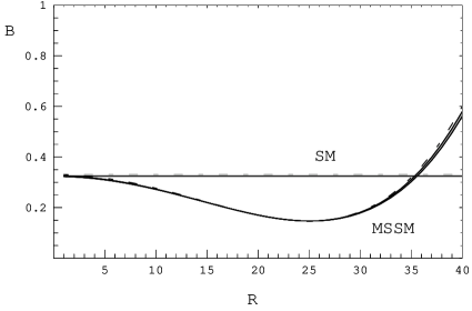
Figure 1: (a) The ratio $B$ as a function of $R$ at $\rho_{1}^{2}=1.33$ in the MSSM and the SM. The lines with shaded region are obtained by using $\Lambda_{\overline{\rm MS}}=0.15\sim 0.25$ GeV and the dashed lines show the predictions without QCD corrections. (b) The ratio of $B$ with and without QCD corrections, $B$(with QCD corrections)/$B$(without QCD corrections), as a function of $R$. The solid and the dashed lines are the ratios with $\Lambda_{\overline{\rm MS}}=0.25$ and $0.15$ GeV.

Fig. 1(a) is the plot of our prediction of the ratio in Eq. (22) as a function of $R$, which is defined by $R\equiv m_{W}\tan\beta/m_{H}$. Here, we do not show the error in the slope parameter $\rho_{1}^{2}$ and we take $\rho_{1}^{2}=1.33$. The dashed lines show the MSSM and SM predictions without QCD corrections. The lines with narrow shaded regions show the predictions including QCD corrections with $\Lambda_{\overline{\rm MS}}$ being varied between 0.15 GeV and 0.25 GeV.

In Fig. 1(b) we show the ratio of $B$ in the MSSM with and without QCD corrections, $B$(with QCD corrections)/$B$(without QCD corrections), as a function of $R$. The solid line is the ratio with $\Lambda_{\overline{\rm MS}}=0.25$ GeV and the dashed line is that with $\Lambda_{\overline{\rm MS}}=0.15$ GeV.

From Fig. 1, we expect that theoretical uncertainties from higher order QCD corrections are at most a few percents in the ratio of decay rates and, as seen later, the theoretical uncertainties from QCD corrections are much smaller than those from the error of $\rho_{1}^{2}$.

Fig. 2(a) shows our prediction of the ratio $B$ with QCD corrections as a function of $R$. Here, we take the error in the slope parameter into account and use $\Lambda_{\overline{\rm MS}}=0.25$ GeV. The shaded regions show the MSSM and SM predictions with the error in the slope parameter $\rho_{1}^{2}$ in Eq. (21). As mentioned before, from Fig. 2(a) and Fig. 1, we see that the theoretical uncertainty from the error in the slope parameter is dominant over that from QCD corrections. As seen in Fig. 1(a), when $R$ is about 35, the ratio $B$ in the MSSM is the same as the one in the SM.

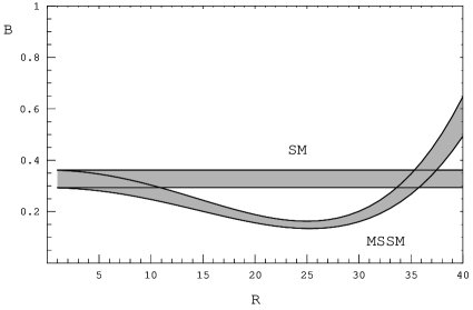
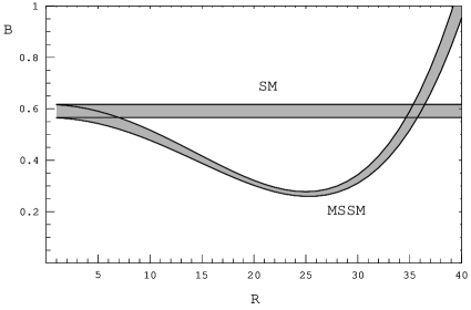
Figure 2: The ratios $B$ and $\tilde{B}$ with QCD corrections as functions of $R$ in the MSSM and the SM. The shaded regions show the predictions with the error in the slope parameter $\rho_{1}^{2}$ in Eq. (21). The flat bands show the SM predictions. (a) $B$: the decay rate normalized to $\Gamma(\bar{B}\rightarrow D\mu\bar{\nu}_{\mu})_{SM}$. (b) $\tilde{B}$: the same as (a) except that the denominator is integrated over $m_{\tau}^{2}\leq q^{2}\leq(m_{B}-m_{D})^{2}$.

In Fig. 2(b), we also show the ratio,

$$\tilde{B}=\frac{\Gamma(\bar{B}\rightarrow D\tau\bar{\nu}_{\tau})}{\tilde{\Gamma}(\bar{B}\rightarrow D\mu\bar{\nu}_{\mu})_{SM}}\;,$$ (23)

with QCD corrections, similar as Fig. 2(a), but its denominator is $\tilde{\Gamma}(\bar{B}\rightarrow D\mu\bar{\nu}_{\mu})_{SM}$, which is integrated over the same $q^{2}$ region as the $\tau$ mode, i.e., $m_{\tau}^{2}\leq q^{2}\leq(m_{B}-m_{D})^{2}$. From Fig. 2(b), we observe that the ratio $\tilde{B}$ has less theoretical uncertainty and we expect a better sensitivity than the ratio $B$ in Fig. 2(a).

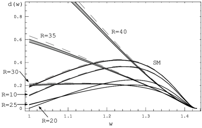
Figure 3: The $w$ distribution $d(w)$ in the SM and the MSSM with different values of $R$. The lines with shaded regions are given by using $\Lambda_{\overline{\rm MS}}=0.15\sim 0.25$ GeV and the dashed lines show the prediction without QCD corrections.

Now, we consider a decay distribution defined by

$$d(w)=(w^{2}-1)\frac{\Gamma(\bar{B}\rightarrow D\tau\bar{\nu}_{\tau})/dw}{\Gamma(\bar{B}\rightarrow D\mu\bar{\nu}_{\mu})_{SM}/dw}\;,$$ (24)

where $w=(m_{B}^{2}+m_{D}^{2}-q^{2})/2m_{B}m_{D}$.

In Fig. 3, we show $d(w)$ in the SM and the MSSM with different values of $R$. The dashed lines show the MSSM and SM predictions without QCD corrections. The lines with shaded regions show the predictions with QCD corrections and the shaded regions are given by using $\Lambda_{\overline{\rm MS}}=0.15\sim 0.25$ GeV. The theoretical uncertainty from the error in the slope parameter is canceled out in this quantity. Thus, QCD corrections become dominant uncertainties in the theoretical calculation. From Fig. 2, the ratio $B$ in the MSSM becomes the same as the one in the SM when $R\sim 35$. But, in Fig. 3, we find that the behavior of $d(w)$ in the MSSM with $R=35$ is considerably different from that in the SM. Therefore, we can distinguish the SM from the MSSM by investigating $w$ distribution even if $R\sim 35$.

5 Conclusion

As seen in our numerical results, the branching ratio of $\bar{B}\rightarrow D\tau\bar{\nu}_{\tau}$ is a sensitive probe of the MSSM-like Higgs sector. So, if $\bar{B}\rightarrow D\tau\bar{\nu}_{\tau}$ is observed at a B factory experiment, a significant region of the parameter space of the MSSM Higgs sector will be proved. This is complementary at the Higgs search at LHC [17].

In the branching ratio, the theoretical uncertainty from QCD correction is much smaller than that from the error in the slope parameter $\rho_{1}^{2}$. However, in $w$ distribution, the theoretical uncertainty from the error in the slope parameter $\rho_{1}^{2}$ is canceled out and, therefore, it is important to consider QCD corrections.

In this work, we have not taken $1/m$ corrections into account. They may be as significant as QCD corrections in the $w$ distribution. However we expect that their effects are smaller than the uncertainty from the error of $\rho_{1}^{2}$ in the branching ratio [10].

Finally, the $\tau$ polarization in $\bar{B}\rightarrow D\tau\bar{\nu}_{\tau}$ is also expected to be a good probe of charged Higgs boson. The theoretical uncertainty from the error in the slope parameter becomes very small in the $\tau$ polarization [3]. QCD and $1/m$ corrections to this quantity will be addressed elsewhere.

Appendix

Functions in Eq. (18) and Eq. (19) are given by

$$r(w) = \frac{1}{\sqrt{w^{2}-1}}\ln(w+\sqrt{w^{2}-1})\;,$$ (A.1)

$$f(w) = wr(w)-2-\frac{w}{2\sqrt{w^{2}-1}}\Big{[}L_{2}(1-w_{-}^{2})-L_{2}(1-w_{+}^{2})\Big{]}\;,$$ (A.2)

$$g_{s}(z,w) = \frac{w}{\sqrt{w^{2}-1}}\Big{[}L_{2}(1-zw_{-})-L_{2}(1-zw_{+})\Big{]}$$ (A.3)

$$-\frac{z}{1-2wz+z^{2}}\Big{[}(w^{2}-1)r(w)+(w-z)\ln z\Big{]}\;,$$

$$a_{L}(w) = \frac{8}{27}\Big{[}wr(w)-1\Big{]}\;,$$ (A.4)

$$Z(w) = -\frac{4}{9}\Big{[}\frac{25}{54}+\frac{\pi^{2}}{12}+\frac{5}{9}+f(w)\Big{]}\Big{[}wr(w)-1\Big{]}-\frac{8}{9}I(w)\;,$$ (A.5)

$$\tilde{Z} = -\frac{7}{225}\pi^{2}-\frac{9403}{7500}\;,$$ (A.6)

where $z=m_{c}/m_{b}$, $w_{\pm}=w\pm\sqrt{w^{2}-1}$,

$$L_{2}(x)=-\int_{0}^{x}dt\frac{\ln(1-t)}{t}\;,$$ (A.7)

is the dilogarithm and,

$$I(w) = \int^{\varphi}_{0}d\psi\Big{[}\psi\coth\psi-1\Big{]}$$ (A.8)

$$\times\Big{\{}\psi\coth^{2}\varphi+\frac{\sinh\varphi\cosh\varphi}{\sinh^{2}\varphi-\sinh^{2}\psi}\ln\frac{\sinh\varphi}{\sinh\psi}\Big{\}}\;,$$

in terms of the hyperbolic angle $\varphi$ defined by $w=\cosh\varphi$.