20+ years of Inflation

Abstract

In this talk I will review the present status of inflationary cosmology and its emergence as the basic paradigm behind the Standard Cosmological Model, with parameters determined today at better than 10% level from CMB and LSS observations. I will also discuss the recent theoretical developments on the process of reheating after inflation and model building based on string theory and D-branes.

1 INTRODUCTION

Until recently, inflation [1] was considered a wild idea, seen with skepticism by many high energy physicists and most astrophysicists. Thanks to the recent observations of the cosmic microwave background (CMB) anisotropies and large scale structure (LSS) galaxy surveys, it has become widely accepted by the community and is now the subject of texbooks [2] and graduate courses. Furthermore, a month ago, the proponents of the idea were awarded the prestigious Dirac Medal for it [3].

In this short review I will outline the reasons why the inflationary paradigm has become the backbone of the present Standard Cosmological Model. It gives a framework in which to pose all the basic cosmological questions: what is the shape and size of the universe, what is the matter and energy content of the universe, where did all this matter come from, what is the fate of the universe, etc. I will describe the basic predictions that inflation makes, most of which have been confirmed only recently, while some are imminent, and then explore the recent theoretical developments on the theory of reheating after inflation and cosmological particle production, which might allow us to answer some of the above questions in the future.

Although the simplest slow-roll inflation model is consistent with the host of high precision cosmological observations of the last few years, we still do not know what the true nature of the inflaton is: although there are many possible realizations, there is no unique particle physics model of inflation. Furthermore, we even ignore the energy scale at which this extraordinary phenomenon occurred in the early universe; it could be associated with a GUT theory or even with the EW theory, at much lower energies.

In the last section, I will describe a recent avenue of proposals for the origin of inflation based on string theory and, in particular, on extended multidimensional objects called D-branes. Whether these ideas will be the seed for the final theory of inflation nobody knows, but it opens up many new possibilities, and even a new language for the early universe, that makes them certainly worthwhile exploring.

2 BASIC PREDICTIONS OF INFLATION

Inflation is an extremely simple idea based on the early universe dominance of a vacuum energy density associated with a hypothetical scalar field called the inflaton. Its nature is not known: whether it is a fundamental scalar field or a composite one, or something else altogether. However, one can always use an effective description in terms of a scalar field with an effective potential driving the quasi-exponential expansion of the universe. This basic scenario gives several detailed fundamental predictions: a flat universe with nearly scale-invariant adiabatic density perturbations with Gaussian initial conditions.

2.1 A flat and homogeneous background

Inflation explains why our local patch of the universe is spatially flat, i.e. Euclidean. Such a (geometrical) property is unstable under the evolution equations of the Big Bang theory in the presence of ordinary matter and radiation [2], making it very unlikely today, unless some new mechanism in the early universe, prior to the radiation era (at least as far back as primordial nucleosynthesis) prepared the universe with such a peculiar initial condition. That is precisely what inflation does, and very efficiently in fact, by providing an approximately constant energy density that induces a tremendous expansion of the universe. Thus, an initially curved three-space will quickly become locally indistinguishable from a “flat” hypersurface. Moreover, this same mechanism explains why we see no ripples, i.e. no large inhomogeneities, in the space-time fabric, e.g. as large anisotropies in the temperature field of the cosmic microwave background when we look in different directions. The expansion during inflation erases any prior inhomogeneities.

These two are very robust predictions of inflation, and constitute the 0-th order, i.e. the space-time background, in a linear expansion in perturbation theory. They have been confirmed to high precision by the detailed observations of the CMB, first by COBE (1992) [4] for the large scale homogeneity, to one part in $10^{5}$, and recently by BOOMERanG [5] and MAXIMA [6], for the spatial flatness, to better than 10%.

2.2 Cosmological perturbations

Inflation also predicts that on top of this homogeneous and flat space-time background, there should be a whole spectrum of cosmological perturbations, both scalar (density perturbations) and tensor (gravitational waves). These arise as quantum fluctuations of the metric and the scalar field during inflation, and are responsible for a scale invariant spectrum of temperature and polarization fluctuations in the CMB, as well as for a stochastic background of gravitational waves. The temperature fluctuations were first discovered by COBE and later confirmed by a host of ground and balloon-borne experiments, while the polarization anisotropies have only recently been discovered by the CMB experiment DASI [7]. Both observations seem to agree with a nearly scale invariant spectrum of perturbations. It is expected that the stochastic background of gravitational waves produced during inflation could be detected with the next generation of gravitational waves interferometers (e.g. LISA), or indirectly by measuring the power spectra of polarization anisotropies in the CMB by the future Planck satellite [8].

Inflation makes very specific predictions as to the nature of the scalar perturbations. In the case of a single field evolving during inflation, the perturbations are predicted to be adiabatic, i.e. all components of the matter and radiation fluid should have equal density contrasts, due to their common origin. As the plasma (mainly baryons) falls in the potential wells of the metric fluctuations, it starts a series of acoustic compressions and rarefactions due to the opposing forces of gravitational collapse and radiation pressure. Adiabatic fluctuations give a very concrete prediction for the position and height of the acoustic peaks induced in the angular power spectrum of temperature and polarization anisotropies. This has been confirmed to better than 1% by the recent observations, and constitutes one of the most important signatures in favor of inflation, ruling out a hypothetically large contribution from active perturbations like those produced by cosmic strings or other topological defects.

Furthermore, the quantum origin of metric fluctuations generated during inflation allows one to make a strong prediction on the statistics of those perturbations: inflation stretches the vacuum state fluctuations to cosmological scales, and gives rise to a Gaussian random field, and thus metric fluctuations are in principle characterized solely by their two-point correlation function. Deviations from Gaussianty would indicate a different origin of fluctuations, e.g. from cosmic defects. Recent observations by BOOMERanG in the CMB and by gravitational lensing of LSS indicate that the non-Gaussian component of the temperature fluctuations and the matter distribution on large scales is strongly constrained, and consistent with foregrounds (in the case of CMB) and with non-linear gravitational collapse (in the case of LSS).

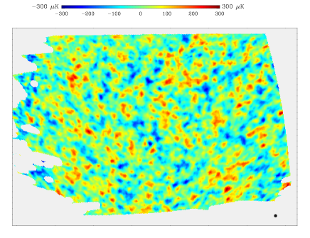
Figure 1: The CMB temperature fluctuations as seen by BOOMERanG. The 1 degree features corresponding to the first acoustic peak are clearly distinguishable. From Ref. [5].

Of course, in order to really confirm the idea of inflation one needs to find cosmological observables that will allow us to correlate the scalar and the tensor metric fluctuations with one another, since they both arise from the same inflaton field fluctuations. This is a daunting task, given that we ignore the absolute scale of inflation, and thus the amplitude of tensor fluctuations (only sensitive to the total energy density). The smoking gun could be the observation of a stochastic background of gravitational waves by the future gravitational wave interferometers and the subsequent confirmation by detection of the curl component of the polarization anisotropies of the CMB. Although the gradient component has recently been detected by DASI, we may have to wait for Planck for the detection of the curl component.

3 RECENT COSMOLOGICAL OBSERVATIONS

Cosmology has become in the last few years a phenomenological science, where the basic theory (based on the hot Big Bang model after inflation) is being confronted with a host of cosmological observations, from the microwave background to the large scale distribution of matter, from the determination of light element abundances to the detection of distant supernovae that reflect the acceleration of the universe, etc. I will briefly review here the recent observations that have been used to define a consistent cosmological standard model.

3.1 Cosmic Microwave Background

The most important cosmological phenomenon from which one can extract essentially all cosmological parameters is the microwave background and, in particular, the last scattering surface temperature and polarization anisotropies, see Fig. 1. Since they were discovered by COBE in 1992, the temperature anisotropies have lived to their promise. They allow us to determine a whole set of both background (0-th order) and perturbation (1st-order) parameters – the geometry, topology and evolution of space-time, its matter and energy content, as well as the amplitude and tilt of the scalar and tensor fluctuation power spectra – in some cases to better than 10% accuracy.

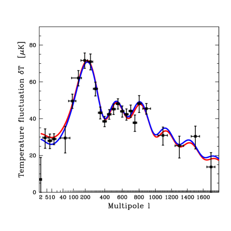
Figure 2: The angular power spectrum of CMB temperature anisotropies. Data includes the recent measurements of BOOMERanG, MAXIMA, DASI, VSA and CBI, as well as a binning of previous measurements, inluding COBE’s. The lines correspond to the theoretical expectation for the $\Lambda$CDM concordance model of [9] (red) and [10] (blue). From Ref. [11].

At present, the forerunners of CMB experiments are two balloons – BOOMERanG [12] and MAXIMA [13] – and three ground based interferometers – DASI [14], VSA [15] and CBI [16]. Together they have allowed cosmologists to determine the angular power spectrum of temperature fluctuations down to multipoles 1000 and 3000, respectively, and therefore provided a measurement of the positions and heigths of at least 3 to 7 acoustic peaks, see Fig. 2. A combined analysis of the different CMB experiments yields convincing evidence that the universe is flat, with $|\Omega_{K}|=|1-\Omega_{\rm tot}|<0.05$ at 95% c.l.; full of dark energy, $\Omega_{\Lambda}=0.66\pm 0.06$, and dark matter, $\Omega_{m}=0.33\pm 0.07$, with about 5% of baryons, $\Omega_{b}=0.05\pm 0.01$; and expanding at a rate $H_{0}=68\pm 7$ km/s/Mpc, all values given with $1\sigma$ errors, see Table 1. The spectrum of primordial perturbations that gave rise to the observed CMB anisotropies is nearly scale-invariant, $n_{s}=1.02\pm 0.06$, adiabatic and Gaussian distributed. This set of parameters already constitutes the basis for a truly Standard Model of Cosmology, based on the Big Bang theory and the inflationary paradigm. Note that both the baryon content and the rate of expansion determinations with CMB data alone are in excellent agreement with direct determinations from BBN light element abundances [17] and HST Cepheids [18], respectively.

Table 1: Estimates of the cosmological parameters that characterize a minimal adiabatic inflation-based model. From Ref. [16].

	Priors	$\Omega_{tot}$	$n_{s}$	$\Omega_{b}\,h^{2}$	$\Omega_{cdm}\,h^{2}$	$\Omega_{\Lambda}$	$\Omega_{m}$	$\Omega_{b}$	$h$	Age	$\tau_{c}$
	CMB	$1.05^{0.05}_{0.05}$	$1.02^{0.06}_{0.07}$	$0.023^{0.003}_{0.003}$	$0.13^{0.03}_{0.02}$	$0.54^{0.12}_{0.13}$	$0.52^{0.15}_{0.15}$	$0.080^{0.023}_{0.023}$	$0.55^{0.09}_{0.09}$	$15.0^{1.1}_{1.1}$	$0.16^{0.18}_{0.13}$
	CMB+LSS	$1.03^{0.03}_{0.04}$	$1.00^{0.06}_{0.06}$	$0.023^{0.003}_{0.003}$	$0.12^{0.02}_{0.02}$	$0.61^{0.09}_{0.10}$	$0.42^{0.12}_{0.12}$	$0.067^{0.018}_{0.018}$	$0.60^{0.09}_{0.09}$	$14.7^{1.2}_{1.2}$	$0.09^{0.12}_{0.07}$
	CMB+LSS+SN	$1.00^{0.03}_{0.02}$	$1.03^{0.06}_{0.06}$	$0.024^{0.003}_{0.003}$	$0.12^{0.02}_{0.02}$	$0.69^{0.04}_{0.06}$	$0.32^{0.06}_{0.06}$	$0.052^{0.011}_{0.011}$	$0.68^{0.06}_{0.06}$	$13.8^{0.9}_{0.9}$	$0.13^{0.14}_{0.10}$
	CMB+LSS+SN+HST	$1.00^{0.02}_{0.02}$	$1.04^{0.05}_{0.06}$	$0.024^{0.002}_{0.003}$	$0.12^{0.01}_{0.01}$	$0.70^{0.02}_{0.03}$	$0.30^{0.02}_{0.02}$	$0.049^{0.004}_{0.004}$	$0.69^{0.02}_{0.02}$	$13.6^{0.2}_{0.2}$	$0.13^{0.13}_{0.10}$

The age of the Universe is in Gyr, and the rate of expansion in units of 100 km/s/Mpc. All values quoted with $1\sigma$ errors.

In the near future, a new satellite experiment, the Microwave Anisotropy Probe (MAP) [19], will provide a full-sky map of temperature (and possibly also polarization) anisotropies and determine the first 2000 multipoles with unprecedented accuracy. When combined with LSS and SN measurements, it promises to allow the determination of most cosmological parameters with errors down to the few% level.

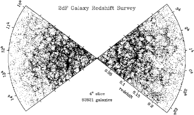
Figure 3: The galaxy distribution of the 2dFGRS, drawn from a total of 221283 galaxies (15 May 2002) in slices $4^{\circ}$ thick, centered at declination $-2.5^{\circ}$ in the NGP and $-27.5^{\circ}$ in the SGP. From Ref. [20].

Moreover, with the recent detection of microwave background polarization anisotropies by DASI [7], confirming the basic paradigm behind the Cosmological Standard Model, a new window opens which will allow yet a better determination of cosmological parameters, thanks to the very sensitive (0.1$\mu$K) and high resolution (4 arcmin) future satellite experiment Planck [8]. In principle, Planck should be able to detect not only the gradient component of the CMB polarization, but also the curl component, if the scale of inflation is high enough. In that case, there might be a chance to really test inflation through cross-checks between the scalar and tensor spectra of fluctuations, which are predicted to arise from the same inflaton potential.

The observed positions of the acoustic peaks of the CMB anisotropies strongly favor purely adiabatic density perturbations, as arise in the simplest single-scalar-field models of inflation. These models also predict a nearly Gaussian spectrum of primordial perturbations. A small degree of non-gaussianity may arise from self-coupling of the inflaton field (although it is expected to be very tiny, given the observed small amplitude of fluctuations), or from two-field models of inflation. Since the CMB temperature fluctuations probe directly primordial density perturbations, non-gaussianity in the density field should lead to a corresponding non-gaussianity in the temperature maps. However, recent searches for non-Gaussian signatures in the CMB have only given stringent upper limits, see Ref. [21].

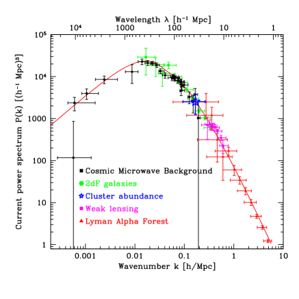
Figure 4: The matter power spectrum. It includes data from the CMB, the matter distribution as seen by 2dFGRS, the cluster abundance, weak gravitational lensing, and Lyman-$\alpha$ forest data. From Ref. [11].

One of the most interesting aspects of the present progress in cosmological observations is that they are beginning to probe the same parameters or the same features at different time scales in the evolution of the universe. We have already mentioned the determination of the baryon content, from BBN (light element abundances) and from the CMB (acoustic peaks), corresponding to totally different physics and yet giving essentially the same value within errors. Another example is the high resolution images of the CMB anisotropies by CBI [16], which constitute the first direct detection of the seeds of clusters of galaxies, the largest gravitationally bound systems in our present universe. In the near future we will be able to identify and put into one-to-one correspondence tiny lumps in the CMB with actual clusters today.

3.2 Large Scale Structure

The last decade has seen a tremendous progress in the determination of the distribution of matter up to very large scales. The present forerunners are the 2dF Galaxy Redshift Survey [22] and the Sloan Digital Sky Survey (SDSS) [23]. These deep surveys aim at $10^{6}$ galaxies and reach redshifts of order 1 for galaxies and order 5 for quasars. They cover a wide fraction of the sky and therefore can be used as excellent statistical probes of large scale structure [20, 24], see Fig. 3.

The main output of these galaxy surveys is the two-point (and higher) spatial correlation functions of the matter distribution or, equivalently, the power spectrum in momentum space. Given a concrete type of matter, e.g. adiabatic vs. isocurvature, cold vs. hot, etc., the theory of linear (and non-linear) gravitational collapse gives a very definite prediction for the measured power spectrum, which can then be compared with observations. This quantity is very sensitive to various cosmological parameters, mainly the dark matter content and the baryonic ratio to dark matter, as well as the universal rate of expansion; on the other hand, it is mostly insensitive to the cosmological constant since the latter has only recently (after redshift $z\sim 1$) started to become important for the evolution of the universe, while galaxies and clusters had already formed by then.

In Fig. 4 we have plotted the measured matter power spectrum with LSS data from the 2dFGRS, plus CMB, weak gravitational lensing and Lyman-$\alpha$ forest data. Together they allow us to determine the power spectrum with better than 10% accuracy for $k>0.02\ h$ Mpc^-1, which is well fitted by a flat CDM model with $\Omega_{m}\,h=0.20\pm 0.03$, and a baryon fraction of $\Omega_{b}/\Omega_{m}=0.15\pm 0.06$, which together with the HST results give values of the parameters that are compatible with those obtained with the CMB.

Figure 5: Likelihood contours for a fit to current CMB data plus the 2dFGRS power spectrum, assuming a flat scalar-dominated model. Note the 10% precision already achieved by cosmological observations. The values of the Hubble parameter and baryon density are in very good agreement with direct estimates. From Ref. [20].

However, the greatest power is attained when combining CMB with LSS, as can be seen in Table 1 and Fig. 5. It is very reassuring to note that present parameter determination is robust as we progress from weak priors to the full cosmological information available, a situation very different from just a decade ago, where the errors were mostly systematic and parameters could only be determined with an order-of-magnitude error. In the very near future such errors will drop again to the 1% level, making Cosmology a mature science, with many independent observations confirming and further constraining previous measurements of the basic parameters.

An example of such progress appears in the analysis of non-Gaussian signatures in the primordial spectrum of density perturbations. The tremendous increase in data due to 2dFGRS and SDSS has allowed cosmologists to probe the statistics of the matter distribution on very large scales and infer from it that of the primordial spectrum. Recently, both groups have reported non-Gaussian signatures (in particular the first two higher moments, skewness and kurtosis), that are consistent with gravitational collapse of structure that was originally Gaussianly distributed [25, 26].

Moreover, weak gravitational lensing also allows an independent determination of the three-point shear correlation function, and there has recently been a claim of detection of non-Gaussian signatures in the VIRMOS-DESCART lensing survey [27], which is also consistent with theoretical expectations of gravitational collapse of Gaussianly distributed initial perturbations.

The recent precise catalogs of the large scale distribution of matter allows us to determine not only the (collapsing) cold dark matter content, but also put constraints on the (diffusing) hot dark matter, since it would erase all structure below a scale that depends on the free streaming length of the hot dark matter particle. In the case of relic neutrinos we have extra information because we know precisely their present energy density, given that neutrinos decoupled when the universe had a temperature around 0.8 MeV and cooled down ever since. Their number density today is around 100 neutrinos/cm³. If neutrinos have a significant mass (above $10^{-3}$ eV, as observations of neutrino oscillations by SuperKamiokande [28] and Sudbury Neutrino Observatory [29] seem to indicate), then the relic background of neutrinos is non-relativistic today and could contribute a large fraction of the critical density, $\Omega_{\nu}=m_{\nu}/92\,h^{2}\!{\rm eV}\geq 0.001$, see Ref. [30]. Using observations of the Lyman-$\alpha$ forest in absorption spectra of quasars, due to a distribution of intervening clouds, a limit on the absolute mass of all species of neutrinos can be obtained [31]. Recently, the 2dFGRS team [32] have derived a bound on the allowed amount of hot dark matter, $\Omega_{\nu}<0.13\,\Omega_{m}<0.05$ (95% c.l.), which translates into an upper limit on the total neutrino mass, $m_{\nu,tot}<1.8$ eV, for values of $\Omega_{m}$ and the Hubble constant in agreement with CMB and SN observations. This bound improves several orders of magnitude on the direct experimental limit on the muon and tau neutrino masses, and is comparable to present experimental bounds on the electron neutrino mass [33].

3.3 Cosmological constant and rate of expansion

Observations of high redshift supernovae by two independent groups, the Supernova Cosmology Project [34], and the High Redshift Supernova Team [35], give strong evidence that the universe is accelerating, instead of decelerating, today. Although a cosmological constant is the natural suspect for such a “crime”, its tiny non-zero value makes theoretical physicists uneasy [36, 37, 38].

A compromise could be found – although to my taste it is rather ugly – by setting the fundamental cosmological constant to zero, by some yet unknown principle possibly related with quantum gravity, and allow a super-weakly-coupled homogeneous scalar field to evolve down an almost flat potential. Such a field would induce an effective cosmological constant that could in principle account for the present observations. The way to distinguish it from a true cosmological constant would be through its equation of state, since such a type of smooth background is a perfect fluid but does not satisfy $p=-\rho$ exactly, and thus $w=p/\rho$ also changes with time. There is a proposal for a satellite called the Supernova / Acceleration Probe (SNAP) [39] that will be able to measure the light curves of type Ia supernovae up to redshift $z\sim 2$, thus determining both $\Omega_{X}$ and $w_{X}$ with reasonable accuracy, where $X$ stands for this hypothetical scalar field. For the moment there are only upper bounds, $w_{X}<-0.6$ (95% c.l.) [40], consistent with a true cosmological constant, but the SNAP project claims it could determine $\Omega_{X}$ and $w_{X}$ with 5% precision.

Fortunately, the SN measurements of the acceleration of the universe give a linear combination of cosmological parameters that is almost orthogonal, in the plane ($\Omega_{m},\ \Omega_{\Lambda}$), to that of the curvature of the universe ($1-\Omega_{K}=\Omega_{m}+\Omega_{\Lambda}$) by CMB measurements and the matter content by LSS data. Therefore, by combining the information from SNe with that of the CMB and LSS, one can significantly reduce the errors in both $\Omega_{m}$ and $\Omega_{\Lambda}$, see Table 1. It also allows an independent determination of the rate of expansion of the universe that is perfectly compatible with the HST data [18]. This is reflected on the fact that adding the latter as prior does not affect significantly the mean value of most cosmological parameters, only the error bars, and can be taken as an indication that we are indeed on the right track: the Standard Cosmological Model is essentially correct, we just have to improve the measurements and reduce the error bars.

4 OTHER PREDICTIONS OF INFLATION

Inflation not only predicts the large scale flatness and homogeneity of the universe and a scale invariant spectrum of metric perturbations. It also implies that all the matter and energy we see in the universe today came from the approximately constant energy density during inflation. The process that converts this energy density into thermal radiation is called reheating of the universe and occurs as the inflaton decay produces particles that rescatter and finally thermalise. In the last decade there has been a tremendous theoretical outburst of activity in this field, thanks to the seminal paper of Kofman, Linde and Starobinsky [41], proposing that reheating could have been preceded by a (short) period of explosive particle production that is extremely non linear, non perturbative and very far from equilibrium. It is this so-called preheating process which is probably responsible for the huge comoving entropy present in our universe. This period is so violent that it may have produced a large stochastic background of gravitational waves [42], which may be detected by future gravitational wave observatories. Such a signature would open up a new window into the very early universe, independently of the late CMB and LSS observations.

4.1 Preheating after inflation

Preheating occurs due to the coherent oscillations of the inflaton at the end of inflation, which induces, through parametric resonance, a short burst of particle production. It is a non-perturbative process very similar to the Schwinger pair production mechanism in quantum electrodynamics. The process of preheating through parametric resonance has been studied in essentially all models of inflation [41], including hybrid inflation [43], and seen to be very generic [44]. Rescattering occurs soon after preheating and thermalization eventually involves all species which are coupled to one another, even if they are not coupled to the inflaton [45]. Nowadays, the full study of this non-perturbative process can only be done with real time numerical lattice simulations [46], performed with a C++ program called LATTICEEASY [47].

Recently, the process of reheating has been studied in the context of theories with spontaneous symmetry breaking [48], and seen to involve strong particle production from the tachyonic growth of the symmetry breaking (Higgs) field [49], and not from the coherent oscillations of the inflaton field. This new process has been denominated as tachyonic preheating [48], and shown to be very efficient in the production of other particles like bosons or fermions that coupled to the Higgs field [50, 51].

4.2 Baryo- and lepto-genesis

This non-perturbative and strongly out of equilibrium stage of the universe could be responsible for one of the remaining mysteries of the universe: the origin of the observed matter-antimatter asymmetry [2], characterised by the conserved ratio of 1 baryon for every $10^{9}$ photons. For the baryon asymmetry of the universe to occur it is necessary (but not sufficient) that the three Sakharov conditions be satisfied: B-violation, C- and CP-violation, and out of equilibrium evolution.

A possible scenario is that of the GUT baryogenesis occurring at the end of inflation through the far from equilibrium stage associated with preheating [52], or even from couplings of the inflaton to R-handed fermions that decay into SM Higgs and leptons, giving rise to a lepton asymmetry [53], which later gets converted into a baryon asymmetry through sphaleron transitions at the electroweak scale, a process known as leptogenesis. Another possibility is that the process of leptogenesis occurs at the end of a hybrid model of inflation, where the couplings of the GUT Higgs field induces strong R-handed fermion production again giving rise to a lepton asymmetry [50].

Moreover, preheating at the electroweak (EW) scale could be sufficiently strongly out of equilibrium to render viable the process of electroweak baryogenesis [54, 55], as long as a new source of CP-violation is assumed at the TeV; see also Ref. [56]. The only assumption needed for preheating to occur at the EW scale is that a short secondary stage of inflation occurs at low energies, as in thermal inflation [57], or through some finetuning of parameters [58]. The CMB anisotropies need not arise from the same stage.

5 MODEL BUILDING

Given the tremendous success that inflationary cosmology is having in explaining the present CMB and LSS observations, it would be desirable that a concrete particle physics model were directly responsible for it. In that case, one could ask many more questions about the model, like couplings to other fields and the decay rate of the inflaton, which would be directly related to the final reheating temperature and the process of preheating. For the moment the CMB observations do not give us much clues, although in the near future, with the MAP satellite, and certainly with Planck, knowledge of the spectral index of density perturbations, and a possible presence of a tensor (gravitational wave) component in the polarization anisotropies, will constraint tremendously the different models already proposed. It is therefore the challenge of theoretical cosmologists to come up now with new proposals for models of inflation that can withstand the expected level of accuracy from future observations.

5.1 hybrid inflation

Perhaps the best motivated model of inflation, from the point of view of particle physics, is hybrid inflation [43]. It is the simplest posible extension of a symmetry breaking (Higgs) field coupled to a singlet scalar that evolves along its slow-roll potential driving inflation with the false vacuum energy of the Higgs field. Inflation ends as the inflaton slow-rolls below a critical value that produces a change of sign of the Higgs’ effective mass squared, from positive to negative, triggering spontaneous symmetry breaking through spinodal instability [44, 59, 51, 49]. In most models the end of inflation occurs in less than one e-fold, and the false vacuum energy decays into radiation through tachyonic preheating [48]. In others there are still a few e-folds after the bifurcation point, and a large peak appears in the power spectrum of density fluctuations [60], which could be responsible for primordial black hole formation [61]. Preheating in hybrid inflation was first studied in Ref. [44], where both types of models were considered and shown to be very different in the process of reheating the universe. This may help distinguish them in the future.

Hybrid inflation has a natural realization in the context of supersymmetric theories, both in D-term and F-term type models [58]. It has the advantage that the values of the fields during inflation are well below the Planck scale, so that supergravity corrections can be safely ignored [62]. Moreover, in susy hybrid inflation it is possible to compute the radiative corrections and show that inflation occurs along the 1-loop Coleman-Weinberg effective potential [63]. Preheating in a concrete susy hybrid inflation model was studied in Ref. [64].

5.2 String theory and D-branes

String theory as a theory of everything and, in particular, as a theory of quantum gravity [65], is a natural framework in which to search for a fundamental theory of inflation. After many years such a search had not been very successful, because the low energy effective theory of strings does not contain any natural candidate for an inflaton field with a sufficiently flat potential to ensure agreement with CMB observations. Only recently, with the advent of D-branes as non-perturbative extended objects in string theory, has there been some progress towards a theory of inflation based on string theory [66]. The most striking characteristic of brane inflation is the geometrical interpretation of the inflaton: it is not a field in the spectrum of strings but the coordinate distance between two D-branes or two orientifold planes in the internal (compactified) space. The scalar potential driving inflation is exactly computable from the 1-loop exchange of open string modes or, equivalently, from the tree level exchange of closed string modes like the graviton, dilaton, etc. In the limit of large distances between the branes (in units of the string length) the potential reduces to the “Newtonian” potential of a supergravity theory due to the exchange of the massless modes of the theory in the compact dimensions,

$$V(y)=V_{0}-\beta/y^{d_{\perp}-2}$$ (1)

where $V_{0}$ is the tree level exchange, the false vacuum energy driving inflation, $y$ is the distance between branes/orientifolds, which plays the role of the inflaton, $d_{\perp}$ is the number of transverse dimensions to the brane in the compactified space, and $\beta$ is a constant that depends on the string coupling, the number of massless fields exchanged and the orientation of the branes. In early models of brane inflation it was necessary to finetune the coupling $\beta$ in order to have enough e-folds of inflation [66]. Last year we proposed a solution [67] by tilting slightly the relative orientation of the branes through a small angle $\theta$ related to supersymmetry breaking in the bulk. In that case, the coupling $\beta$ is naturally small and a successful inflation is ensured. The potential is attractive and the two branes approach eachother. When the branes are close enough, compared with the string scale, there appears a tachyon in the spectrum of the strings, whose effective potential develops a minimum and a true vacuum. Inflation ends when the inflaton changes the sign of the tachyon mass squared and triggers symmetry breaking.

Figure 6: The inflaton field is interpreted as the distance $y$ between the two branes. Quantum fluctuations of this field will give rise upon collision to density perturbations on comoving hypersurfaces. These fluctuations will be later observed as temperature anisotropies in the microwave background. From Ref. [67].

Table 2: Correspondences between ordinary and brane inflation.

Quantum Field Theory	D-Brane/String Theory
Scalar field $\phi$	Distance between branes $\ y$
Potential $V(\phi)$	Tree-level + 1-loop exchange of string modes (1)
Slow-roll parameters	Slow-roll parameters
$\epsilon={\displaystyle{M_{\rm P}^{2}\over 2}\left({V^{\prime}\over V}\right)^{2}}$	$\epsilon={\displaystyle{3v^{2}\over 4}}$                         relative velocity of the branes
$\eta={\displaystyle M_{\rm P}^{2}\,{V^{\prime\prime}\over V}}$	$\eta={\displaystyle-{d_{\perp}-1\over d_{\perp}N}}$                  relative acceleration of the branes
$n=1+2\eta-6\epsilon$	${\displaystyle n=1-{2(d_{\perp}-1)\over d_{\perp}N}}$           fixed by dimensions of compatified space
Number of $e$-folds
$N={\displaystyle{1\over M_{\rm P}}\int{V\,d\phi\over V^{\prime}(\phi)}}$	$N={\displaystyle{H\over v}\int\!dy}$                   integrated distance between branes
Quantum Fluctuations
${\cal R}_{k}={\displaystyle{\delta\rho_{k}\over\dot{\rho}}=H\,{\delta\phi_{k}\over\dot{\phi}}}$	${\cal R}_{k}={\displaystyle\delta N_{k}={H\over v}\,\delta y_{k}}$          spatial fluctuations in the branes

From the point of view of model building this model is very similar to hybrid inflation; in fact, it is probably the first concrete realization of hybrid inflation in the context of string theory [67, 68]. The main difference is that we do not have here a complicated field theory with an a priori undetermined scalar potential; on the contrary, the field content and the string dynamics is automatically determined by the brane configuration in the compactified space. This model predicts that the inflaton is massless while its potential is given by an inverse power law. The usual slow-roll parameters have here very clear geometrical interpretations as the relative velocity and acceleration of the branes, and the number of e-folds is determined by the integrated distance between the branes: the further apart the branes are initially, the bigger the number of e-folds of inflation. See Table 2 for the general dictionary between the usual inflationary parameters and the brane inflation ones. In a sense, the model [67] is very robust with respect to initial conditions and it is not necessary to finetune these in order to have inflation, see Ref. [66].

The geometrical correspondence goes one step further when studying quantum fluctuations and the origin of density perturbations. In ordinary inflation, it is the fluctuations of the inflaton field that determine the metric fluctuations through the Einstein equations. In these brane models, inflation ends when the two branes approach eachother and collide, and the spatial fluctuations of the brane itself (a sheet in some extra dimensional space) implies that inflation ends at different times in different points of the (3+1)-brane, directly giving rise to metric fluctuations.

The amplitude and tilt of CMB anisotropies in brane inflation models determines both the string scale and the compactification scale to be of order $10^{13}$ GeV, slightly lower than usual GUT theories, although the whole idea of GUT unification has to be revised in the context of these brane models. Therefore, the model typically predicts a negligible amplitude for the tensor component in the polarization power spectra that may escape detection even by Planck. On the other hand, the scalar tilt is predicted to be $n=1-2(d_{\perp}-1)/(d_{\perp}N)=0.974$, with $d_{\perp}=4$ and $N=60$ as in Ref. [67]. This is so precise that the next generation of CMB experiments will very easily rule out this model in case observations do not agree with this value.

6 CONCLUSIONS

After 20+ years, inflation is a robust paradigm with a host of cosmological observations confirming many of its basic predictions: large scale spatial flatness and homogeneity, as well as an approximately scale-invariant Gaussian spectrum of adiabatic density perturbations.

It is possible that in the near future the next generation of CMB satellites (MAP and Planck) may detect the tensor or gravitational wave component of the polarization power spectrum, raising the possibility of really testing inflation through the comparison of the scalar and tensor components, as well as determining the energy scale of inflation.

The stage of reheating, and more specifically preheating, after inflation is today one of the most active areas of research in theoretical cosmology, with the expectation that it may contain clues to the actual origin of the matter-antimatter asymmetry and be responsible for signatures, like a stochastic background of gravitational waves, that may open a new window to the early universe beyond that of Big Bang Nucleosynthesis.

Although inflation is a very beautiful and elegant paradigm, there is still no compelling particle physics model for it, while the scale of inflation is still uncertain. Hybrid inflation is a particularly nice realization that comes almost for free with any particle physics model of spontaneous symmetry breaking, be it GUT, intermediate of EW scale, by assuming a light singlet (the inflaton) coupled to the symmetry breaking field.

String theory has recently provided for a concrete realization of inflation in the context of D-brane interactions mediated by open or closed strings. It is in fact an interesting hybrid inflation model, where the string tachyon plays the role of the symmetry breaking field that triggers the end of inflation. This model is robust and gives specific predictions for the amplitude and tilt of the spectrum of metric fluctuations, which will soon be tested against precise observations of the microwave background anisotropies.

References

- [1] A. H. Guth, Phys. Rev. D 23 (1981) 347; A. D. Linde, Phys. Lett. B 108 (1982) 389; A. Albrecht and P. J. Steinhardt, Phys. Rev. Lett. 48 (1982) 1220.
- [2] A. D. Linde, Particle Physics and Inflationary Cosmology, Harwood Academic Press (1990); E. W. Kolb and M. S. Turner, The Early Universe, Addison-Wesley (1990); A. R. Liddle and D. H. Lyth, Cosmological Inflation And Large-Scale Structure, Cambridge Univ. Press (2000); J. A. Peacock, Cosmological Physics, Cambridge Univ. Press (1999).
- [3] http://www.ictp.trieste.it/sci_info/ awards/Dirac/DiracMedallists/ DiracMedal02.html
- [4] G. F. Smoot, Astrophys. J. 396 (1992) L1; C. L. Bennett et al., Astrophys. J. 464 (1996) L1.
- [5] P. de Bernardis et al. (Boomerang Collaboration), Nature 404 (2000) 955 [astro-ph/0004404].
- [6] S. Hanany et al., Astrophys. J. 545 (2000) L5 [astro-ph/0005123].
- [7] J. Kovac et al. (DASI Collaboration), “Detection of Polarization in the Cosmic Microwave Background using DASI,” astro-ph/0209478.
-
[8]
Planck home page:
http://astro.estec.esa.nl/Planck/ - [9] X. m. Wang, M. Tegmark and M. Zaldarriaga, Phys. Rev. D 65 (2002) 123001 [astro-ph/0105091].
- [10] G. Efstathiou et al. (2dFGRS Collaboration), Mon. Not. Roy. Astron. Soc. 330 (2002) L29.
- [11] M. Tegmark and M. Zaldarriaga, “Separating the Early Universe from the Late Universe: cosmological parameter estimation beyond the black box,” astro-ph/0207047.
-
[12]
BOOMERANG home page:
http://oberon.roma1.infn.it/boomerang/ -
[13]
MAXIMA home page:
http://cosmology.berkeley.edu/group/cmb/ -
[14]
DASI home page:
http://astro.uchicago.edu/dasi/ - [15] J. A. Rubino-Martin et al. (VSA Collaboration), “First results from the Very Small Array. IV: Cosmological parameter estimation,” astro-ph/0205367.
- [16] J. L. Sievers et al. (CBI Collaboration), “Cosmological Parameters from Cosmic Background Imager Observations and Comparisons with BOOMERanG, DASI, and MAXIMA,” astro-ph/0205387.
- [17] J. M. O’Meara, D. Tytler, D. Kirkman, N. Suzuki, J. X. Prochaska, D. Lubin and A. M. Wolfe, Astrophys. J. 552 (2001) 718 [astro-ph/0011179]; D. Tytler, J. M. O’Meara, N. Suzuki and D. Lubin, “Review of Big Bang Nucleosynthesis and Primordial Abundances,” astro-ph/0001318.
- [18] W. L. Freedman et al., Astrophys. J. 553 (2001) 47 [astro-ph/0012376].
-
[19]
Microwave Anisotropy Prove home page:
http://map.gsfc.nasa.gov/ - [20] J. A. Peacock, “Studying large-scale structure with the 2dF Galaxy Redshift Survey,” astro-ph/0204239.
- [21] G. Polenta et al., Astrophys. J. 572 (2002) L27 [astro-ph/0201133].
- [22] 2dF Galaxy Redshift Survey home page: http://www.mso.anu.edu.au/2dFGRS/
- [23] Sloan Digital Sky Survey home page: http://www.sdss.org/sdss.html
- [24] W. J. Percival et al. (2dFGRS Collaboration), “Parameter constraints for flat cosmologies from CMB and 2dFGRS power spectra,” astro-ph/02006256.
- [25] L. Verde, R. Jimenez, M. Kamionkowski and S. Matarrese, Mon. Not. Roy. Astron. Soc. 325 (2001) 412 [astro-ph/0011180].
- [26] I. Szapudi et al. (SDSS Collaboration), Astrophys. J. 570 (2002) 75 [astro-ph/0111058].
- [27] F. Bernardeau, Y. Mellier, L. van Waerbeke, Astron. & Astrophys. 389 (2002) L28 [astro-ph/0201032].
- [28] Y. Fukuda et al. (SuperK Collaboration), Phys. Rev. Lett. 82 (1999) 2644 [hep-ex/9812014]; Phys. Rev. Lett. 85 (2000) 3999 [hep-ex/0009001].
- [29] Q. R. Ahmad et al. (SNO Collaboration), Phys. Rev. Lett. 89 (2002) 011301 [nucl-ex/0204008]; Phys. Rev. Lett. 89 (2002) 011302 [nucl-ex/0204009].
- [30] W. Hu, D. J. Eisenstein and M. Tegmark, Phys. Rev. Lett. 80 (1998) 5255 [astro-ph/9712057].
- [31] R. A. Croft, W. Hu and R. Dave, Phys. Rev. Lett. 83 (1999) 1092 [astro-ph/9903335].
- [32] O. Elgaroy et al. (2dFGRS Collaboration), Phys. Rev. Lett. 89 (2002) 061301 [astro-ph/0204152].
- [33] Review of particle properties, Particle Data Group home page: http://pdg.web.cern.ch/pdg/
- [34] S. Perlmutter et al. (Supernova Cosmology Project Collaboration), Astrophys. J. 517 (1999) 565 [astro-ph/9812133].
- [35] A. G. Riess et al. (Supernova Search Team Collaboration), Astron. J. 116 (1998) 1009 [astro-ph/9805201].
- [36] S. Weinberg, Rev. Mod. Phys. 61 (1989) 1.
- [37] S. M. Carroll, Living Rev. Rel. 4 (2001) 1 [astro-ph/0004075].
- [38] P. J. Peebles and B. Ratra, “The cosmological constant and dark energy,” astro-ph/0207347.
-
[39]
Supernova / Acceleration Probe home page:
http://http://snap.lbl.gov/ - [40] S. Perlmutter, M. S. Turner and M. J. White, Phys. Rev. Lett. 83 (1999) 670 [astro-ph/9901052].
- [41] L. Kofman, A. Linde and A. A. Starobinsky, Phys. Rev. Lett. 73 (1994) 3195 [hep-th/9405187]; Phys. Rev. D 56 (1997) 3258 [hep-ph/9704452]; P. B. Greene, L. Kofman, A. Linde and A. A. Starobinsky, Phys. Rev. D 56 (1997) 6175 [hep-ph/9705347].
- [42] S. Y. Khlebnikov and I. I. Tkachev, Phys. Rev. D 56 (1997) 653 [hep-ph/9701423].
- [43] A.D. Linde, Phys. Lett. B259 (1991) 38; Phys. Rev. D 49 (1994) 748 [astro-ph/9307002].
- [44] J. García-Bellido and A. D. Linde, Phys. Rev. D 57 (1998) 6075 [hep-ph/9711360].
- [45] G. Felder and L. Kofman, Phys. Rev. D 63 (2001) 103503 [hep-ph/0011160].
- [46] S. Yu. Khlebnikov and I. I. Tkachev, Phys. Rev. Lett. 77 (1996) 219 [hep-ph/9603378]; Phys. Rev. Lett. 79 (1997) 1607 [hep-ph/9610477];
- [47] G. Felder and I.I Tkachev, “LATTICEEASY: A program for lattice simulations of scalar fields in an expanding Universe”, hep-ph/0011159.
- [48] G. N. Felder, J. García-Bellido, P. B. Greene, L. Kofman, A. D. Linde and I. Tkachev, Phys. Rev. Lett. 87 (2001) 011601 [hep-ph/0012142]; G. N. Felder, L. Kofman and A. D. Linde, Phys. Rev. D 64 (2001) 123517 [hep-th/0106179].
- [49] J. García-Bellido, M. García Pérez and A. González-Arroyo, “Symmetry breaking and false vacuum decay after hybrid inflation,” hep-ph/0208228.
- [50] J. García-Bellido and E. Ruiz Morales, Phys. Lett. B 536 (2002) 193 [hep-ph/0109230].
- [51] E. J. Copeland, S. Pascoli and A. Rajantie, Phys. Rev. D 65 (2002) 103517 [hep-ph/0202031].
- [52] E. W. Kolb, A. D. Linde and A. Riotto, Phys. Rev. Lett. 77 (1996) 4290 [hep-ph/9606260].
- [53] G. F. Giudice, M. Peloso, A. Riotto and I. Tkachev, JHEP 9908 (1999) 014 [hep-ph/9905242].
- [54] J. García-Bellido, D. Y. Grigoriev, A. Kusenko and M. E. Shaposhnikov, Phys. Rev. D 60 (1999) 123504 [hep-ph/9902449]
- [55] L. M. Krauss and M. Trodden, Phys. Rev. Lett. 83 (1999) 1502 [hep-ph/9902420].
- [56] A. Rajantie, P. M. Saffin and E. J. Copeland, Phys. Rev. D 63 (2001) 123512 [hep-ph/0012097]; E. J. Copeland, D. Lyth, A. Rajantie and M. Trodden, Phys. Rev. D 64 (2001) 043506 [hep-ph/0103231].
- [57] D. H. Lyth and E. D. Stewart, Phys. Rev. D 53 (1996) 1784 [hep-ph/9510204].
- [58] D. H. Lyth and A. Riotto, Phys. Rept. 314 (1999) 1 [hep-ph/9807278].
- [59] T. Asaka, W. Buchmuller and L. Covi, Phys. Lett. B 510 (2001) 271 [hep-ph/0104037].
- [60] L. Randall, M. Soljacic and A. H. Guth, Nucl. Phys. B 472 (1996) 377 [hep-ph/9512439].
- [61] J. García-Bellido, A. D. Linde and D. Wands, Phys. Rev. D 54 (1996) 6040 [astro-ph/9605094].
- [62] A. D. Linde and A. Riotto, Phys. Rev. D 56 (1997) 1841 [hep-ph/9703209].
- [63] G. R. Dvali, Q. Shafi and R. Schaefer, Phys. Rev. Lett. 73 (1994) 1886 [hep-ph/9406319].
- [64] M. Bastero-Gil, S. F. King and J. Sanderson, Phys. Rev. D 60 (1999) 103517 [hep-ph/9904315].
- [65] J. Polchinski, “String Theory”, 2 Vols. Cambridge Univ. Press (1998).
-
[66]
G. Dvali, S.-H. Henry Tye,
Phys. Lett. B 450 (1999) 72 [hep-ph/9812483];
C.P. Burgess, M. Majumdar, D. Nolte, F. Quevedo, G. Rajesh, R.-J. Zhang, JHEP 0107 (2001) 047 [hep-th/0105204];
G. R. Dvali, Q. Shafi and S. Solganik, hep-th/0105203.
G. Shiu and S. H. Tye, Phys. Lett. B 516 (2001) 421 [hep-th/0106274];
C. Herdeiro, S. Hirano, R. Kallosh, JHEP 0112 (2001) 027 [hep-th/0110271];
B. s. Kyae and Q. Shafi, Phys. Lett. B 526 (2002) 379 [hep-ph/0111101]. - [67] J. García-Bellido, R. Rabadán and F. Zamora, JHEP 0201 (2002) 036 [hep-th/0112147]; J. García-Bellido and R. Rabadán, JHEP 0205 (2002) 042 [hep-th/0203247].
-
[68]
C.P. Burgess, P. Martineau, F. Quevedo, G. Rajesh, R.-J. Zhang,
JHEP 0203 (2002) 052 [hep-th/0111025];
R. Blumenhagen, B. Kors, D. Lüst, T. Ott, Nucl. Phys. B 641 (2002) 235 [hep-th/0202124];
K. Dasgupta, C. Herdeiro, S. Hirano, R. Kallosh, Phys. Rev. D 65 (2002) 126002 [hep-th/0203019];
N. Jones, H. Stoica, S.-H.Henry Tye, JHEP 0207 (2002) 051 [hep-th/0203163].