RELATIVISTIC INSTANT–FORM APPROACH TO THE STRUCTURE OF TWO-BODY COMPOSITE SYSTEMS. II. NONZERO SPIN

Abstract

The relativistic approach to electroweak properties of two-particle composite systems developed in Ref.[1] is generalized here to the case of nonzero spin. This approach is based on the use of the instant form of relativistic Hamiltonian dynamics. The generalization makes use of a special mathematical technique for the parametrization of matrix elements of electroweak current operators in terms of form factors. In this technique the parametrization is a realization of the Wigner–Eckart theorem on the Poincaré group and form factors are reduced matrix elements. As in the case of zero spin the electroweak current matrix element satisfies the relativistic covariance conditions and in the case of electromagnetic current it also automatically satisfies the conservation law. Physical approximations such as, for example, the relativistic impulse approximation, are formulated in terms of reduced matrix elements. The electromagnetic structure of $\rho$ meson is calculated as an example of realization of the technique proposed.

PACS number(s): 13.40.–f, 11.30.Cp

I Introduction

A new relativistic approach to electroweak properties of composite systems has been proposed in our recent paper [1]. The approach is based on the use of the instant form (IF) of relativistic Hamiltonian dynamics (RHD). The detailed description of RHD can be found in the review [2]. Some other references as well as some basic equations of RHD approach are given in Ref.[1].

In the paper [1] our approach was used to perform a realistic calculation of electroweak properties of pion considered as composite quark–antiquark system. The electromagnetic form factor and the lepton decay constant were calculated for pion using different model wave functions for the relative motion of quarks in pion.

Now our aim is to generalize the approach to more complicated systems, namely, to composite systems of two particles of spin 1/2 with nonzero values of total angular momentum, total orbital momentum and total spin. The main problem is a construction of electromagnetic current operator satisfying standard conditions (Lorentz covariance, conservation law etc., see, e.g., Ref.[1]).

The basic point of our approach [1] to the construction of the electromagnetic current operator is the general method of relativistic invariant parameterization of local operator matrix elements proposed as long ago as in 1963 by Cheshkov and Shirokov [3]. This canonical parametrization of local operators matrix elements was generalized to the case of composite systems of free particles in Refs. [4, 5].

In fact, this parametrization is a realization of the Wigner–Eckart theorem for the Poincaré group and so it enables one for given matrix element of arbitrary tensor dimension to separate the reduced matrix elements (form factors) that are invariant under the Poincaré group. The matrix element of a given operator is represented as a sum of terms, each one of them being a covariant part multiplied by an invariant part. In such a representation a covariant part describes transformation (geometrical) properties of the matrix element, while all the dynamical information on the transition is contained in the invariant part – reduced matrix elements. In the case of composite systems these form factors appearing through the canonical parameterization are to be considered in the sense of distributions, that is they are generalized instead of classical functions. As was demonstrated in Ref.[1] this fact takes place even in nonrelativistic case. It is in terms of form factors that the electroweak properties of composite systems are described in the frame of the approach [1].

In our approach some rather general problems arising in the description of composite quark models have been solved. For example, the description of electromagnetic properties of composite systems in terms of form factors in Ref.[1], in fact, solves the problem of construction of the electromagnetic current satisfying the conditions of translation invariance, Lorentz covariance, conservation law, cluster separability and equality of the composite system charge to the sum of constituents charges (charge nonrenormalizability).

Let us note that the importance of the problem of the construction of the electromagnetic current is actual not only for RHD but for all relativistic approaches to composite systems, including the field theoretical approaches [6, 7, 8, 9, 10, 11, 12, 13].

We will construct the electromagnetic current operator in the frame of IF of RHD. The same problem was considered in Refs. [6, 13] in the point form of RHD and in Refs. [11, 12] in the case of light–front dynamics.

Our approach is a generalization of the method [13] to the case of the instant form dynamics. However, the scenario of the generalization of the Wigner–Eckart theorem is quite different.

Physical approximations that we use in our approach are formulated in terms of reduced matrix elements, for example, the well known relativistic impulse approximation. It means that the electromagnetic current of a composite system is a sum of one–particle currents of the constituents. It is worth emphasizing that in our method this approximation does not violate the standard conditions for the current listed before. To–day a construction of relativistic impulse approximation without breaking of relativistic covariance and current conservation law is a common trend of different approaches [6, 10, 11, 13]. Let us note that in the present paper it is for the first time that such a construction has been realized for the case of nonzero spin in the frame of IF RHD. This is a variant of the relativistic impulse approximation (IA) formulated in terms of reduced matrix elements (see Ref. [1]) – the modified impulse approximation (MIA).

The canonical parameterization of electroweak current matrix element, i.e. the extraction of the reduced matrix elements in the case of zero total spin and zero total angular momentum was performed in Ref. [1] and is rather simple. The case of composite systems with nonzero values of total spin and angular momentum requires the development of a general method for canonical parameterization of local operator matrix elements. Here we develop an adequate mathematics using as a base the paper [3].

In the present paper we propose a general formalism for the operators diagonal in the total angular momentum. The case of non-diagonal operators describing, for example, the radiative transitions between vector and scalar composite particles will be considered elsewhere. We demonstrate the application of the formalism in the case of a system with total spin one and total angular momentum one and with zero orbital momentum. In this connection the $\rho$ – meson electromagnetic structure is calculated as an example. Using different model wave functions of the quark relative motion we calculate the electromagnetic form factors and the static properties of the $\rho$ meson supposing quarks to be in the $S$ state of relative motion. It is interesting to mention that relativistic effects occur to produce a nonzero quadrupole momentum and quadrupole form factor. It is well known that in the nonrelativistic case the non–zero quadrupole form factor is caused by the presence of the $D$- wave and is zero otherwise.

It is worth noticing that our approach guarantees the uniqueness of the solution for the $\rho$ – meson electromagnetic form factors in contrast with the calculations based on the standard light–front dynamics in Refs. [14, 15] where it is shown that the form factors obtained from matrix elements with different total angular momentum projections differ from one another themselves. An analogous ambiguity takes place in the light-front dynamics calculations of the deuteron electromagnetic structure [16]. The next step of generalization of our approach concerns two–particle systems with nonzero orbital momentum giving a possibility to describe this simplest nuclear composite system [17].

The paper is organized as follows. In Sec.II the canonical parametrization of local operator matrix elements between one–particle states of arbitrary nonzero spin is described. This parametrization presents the extraction of the reduced matrix element on the Poincaré group. The electromagnetic current matrix element is derived for the spin 1/2 particle. For this case the relations between the form factors in the canonical parametrization form and commonly used Sachs form factors are given explicitly.

In Sec.III we show how to construct the electromagnetic current operator for composite system of two free particles of spin 1/2. The current matrix element is obtained in the basis where the center–of–mass motion is separated. The electromagnetic properties of the system are defined by reduced matrix elements, or the so called free two–particle form factors, these form factors being generalized functions. This means that, for example, the static properties of the system are given by the weak limits as $Q^{2}\to$ 0 ($Q^{2}=-q^{2}\;,\;q$ is the momentum transfer). A special attention is paid to the case of total spin one and zero total orbital momentum. In this case the electromagnetic properties are defined by four free two–particle form factors – charge, quadrupole, magnetic and the magnetic quadrupole form factor of the second kind (see the review in Ref. [18] and the references therein).

In Sec.IV the electromagnetic current matrix element is constructed for the case of two interacting particles. Each step of the calculation in the developed method remains Lorentz covariant and conserves the current. The composite system form factors are derived as some integral representations in terms of the wave functions obtained in the frame of RHD.

In Sec.V the developed formalism is used in the case of the system with total spin one and total angular momentum one. In terms of reduced matrix elements the so called modified impulse approximation (MIA)  [1] is formulated. In MIA $\rho$ – meson form factors are obtained explicitly.

In Sec.VI the results of calculations of static properties and electromagnetic form factors of $\rho$ meson are discussed.

In Sec.VII the conclusion is given.

II Parametrization of one–particle operator matrix elements

A parametrization of the current operator matrix element is a representation of the matrix element in terms of form factors. Let us remark that it is just form factors – Lorentz invariant functions – are extracted from scattering data. In simple cases, such as particles with spin 0 or 1/2 the parametrization can be obtained through semiempirical approaches. However, in more complicated cases, for example, in the case of nuclei with arbitrary spins one needs a general mathematical method.

Let us describe now a general method for canonical parameterization of local operator matrix elements ( see Ref. [3], too). As we have mentioned before, here we are dealing with the matrix elements diagonal in total angular momentum only. Non-diagonal case will be considered elsewhere.

From the group theory point of view a parameterization is, in fact, a realization of the well known Wigner–Eckart theorem on the Poincaré group. The parameterization extracts the reduced matrix elements that are invariant under the Poincaré group. These reduced matrix elements are just form factors that are measured in experiments.

The main idea of the parametrization can be formulated as follows. Using the variables entering the state vectors which define the matrix elements one has to construct two types of objects.

1. A set of linearly independent matrices which are Lorentz scalars (scalars or pseudoscalars). This set describes transition matrix elements non-diagonal in spin projections in the initial and finite states, as well as the properties defined by the discrete space–time transformations.

2. A set of linearly independent objects with the same tensor dimension as the operator under consideration (for example, four–vector, or four–tensor of some rank). This set describes the matrix element behaviors under the action of Lorentz group transformations. In the case of Lorentz scalar operator the second set coincides with the first one.

The operator matrix element is written as a sum of all possible objects of the first type multiplied by all the possible objects of the second type. The coefficients in this representation as a sum are just the reduced matrix elements – form factors. The obtained representation is then modified with the use of additional conditions for the operator, such as the conservation laws, for example. In order to satisfy these additional conditions in some cases some of the coefficients occur to be zero.

To demonstrate this let us consider the parameterization of the matrix elements taken between the states of a free particle of mass $M$ in different simple cases. Let us normalize the state vectors as follows  [1]:

$$\langle\,\!\vec{p}\,,m\,|\,\vec{p}\,^{\prime}\,,m^{\prime}\,\!\rangle=2p_{0}\,\delta(\vec{p}-\vec{p}\,^{\prime})\,\delta_{mm^{\prime}}\;,$$ (1)

Here $\vec{p}\;,\;\vec{p}\,^{\prime}$ are three–momenta of particle, $p_{0}=\sqrt{M^{2}+\vec{p}\,^{2}}$, $m\;,\;m^{\prime}$ are spin projections.

Let us consider first the parameterization of the matrix element of scalar operator $A(x)$ taken between the states of free particle with zero spin. Because of translation invariance it is sufficient to consider $A(0)$. Using the variables of state vectors in the initial and final states one can construct two linearly independent scalars: $p^{2}={p^{\prime}}\,^{2}=M^{2}\;,\;(p-p^{\prime})^{2}=q^{2}=-Q^{2}$. Only the second one – the momentum transfer square – is nontrivial. Ignoring the trivial dependence on $M$ we can write:

$$\langle\,\vec{p},\,M|A(0)|\,\vec{p}\,^{\prime},\,M\,\rangle=f(Q^{2})\;.$$ (2)

Let us consider now the matrix element of a scalar operator between the states of a particle with spin $j$:

$$\langle\,\vec{p},\,M,\,j,\,m\,|A(0)|\,\vec{p}\,^{\prime},\,M,\,j,\,m^{\prime}\,\rangle$$ (3)

The tensor dimension of the operator is not changed, nevertheless, the matrix element is now a matrix in spin projections in the initial and finite states.

Let us construct the set of Lorentz scalars – linearly independent matrices in spin projections to be used for the construction of the representation of Eq. (3). Let us use the covariant spin operator $\Gamma^{\mu}(p)$ [19]. In the rest frame this operator coincides with the particle spin operator:

$$\Gamma^{0}(0)=0\;,\quad\vec{\Gamma}(0)=M\,\vec{j}\;,\quad[\,j_{i}\,,j_{k}\,]=i\,\varepsilon_{ikl}\,j_{l}\;.$$ (4)

The covariant spin operator can be defined with the use of the Pauli-Lubanski vector $w^{\mu}$ [20]. In terms of matrix elements we have:

$$\Gamma^{\mu}_{mm^{\prime}}(p)=\langle\,\vec{p}\,,m|w^{\mu}|\vec{p}\,,m^{\prime}\rangle$$

$$=\langle\,0\,,m|\hat{U}^{-1}(\Lambda_{p})w^{\mu}\hat{U}(\Lambda_{p})|0\,,m^{\prime}\rangle$$ (5)

$$=\left(\Lambda_{p}\right)^{\mu}_{\nu}\langle\,0\,,m|w^{\nu}|0\,,m^{\prime}\rangle=\left(\Lambda_{p}\right)^{\mu}_{\nu}\,\Gamma^{\nu}_{mm^{\prime}}(0)\;.$$

Here $\Lambda_{p}$ is the boost for the transformation from the rest frame of the particle to the laboratory frame, $\hat{U}(\Lambda_{p})$ is the corresponding representation operator. The matrix $\Lambda_{p}$ can be written explicitly using the matrix for Lorentz transformation of the vector $p^{\prime}$ into the vector $p$:

$$\Lambda^{\mu}_{\;\nu}=\delta^{\mu}_{\nu}+\frac{2}{M^{2}}p^{\mu}\,p^{\prime}_{\nu}-\frac{(p^{\mu}+{p^{\prime}}\,^{\mu})(p_{\nu}+p^{\prime}_{\nu})}{M^{2}+p^{\lambda}\,p^{\prime}_{\lambda}}\;.$$ (6)

In our case $\Lambda_{p}$ is given by Eq. (6) with $p^{\prime}=(M\;,\;0\;,\;0\;,\;0)$.

Now equations (4) can be written as:

$$\Gamma^{0}_{mm^{\prime}}(0)=\langle\,0\,,m|w^{0}|0\,,m^{\prime}\rangle=0\;,$$

$$\vec{\Gamma}_{mm^{\prime}}(0)=\langle\,0\,,m|\vec{w}|0\,,m^{\prime}\rangle=M\,\vec{j}_{mm^{\prime}}\;.$$ (7)

Using the explicit form of $\Lambda_{p}$ we obtain:

$$\Gamma_{0}(p)=(\vec{p}\vec{j})\;,\quad\vec{\Gamma}(p)=M\,\vec{j}+\frac{\vec{p}(\vec{p}\vec{j})}{p_{0}+M}\;,$$

$$\quad\Gamma^{2}=-M^{2}\,j(j+1)\;.$$ (8)

As is known [20], spin transforms under the action of Lorentz group following the so called little group which is isomorphic to the rotation group, that is the corresponding transformations are realized by the matrices of three dimensional rotations. The derivation of the explicit form of these matrices with an arbitrary spin is described in Ref. [21]. For spin 1 and 1/2 the matrices have the form:

$$D^{1/2}(p_{1},p_{2})=\cos\frac{\omega}{2}-2\,i\,(\vec{k}\cdot\vec{j})\,\sin\frac{\omega}{2}\;,$$

$$D^{1}(p_{1},p_{2})=I-i(\vec{k}\cdot\vec{j})\,\sin\omega+(\vec{k}\cdot\vec{j})^{2}\,(\cos\omega-1)\;,$$

$$\omega=2\,\arctan\,\frac{|[\,\vec{p}_{1}\,,\vec{p}_{2}\,]|}{(p_{10}+M_{1})(p_{20}+M_{2})-(\vec{p}_{1}\vec{p}_{2})}\;,$$

$$\vec{k}=\frac{[\,\vec{p}_{1}\,,\vec{p}_{2}\,]}{|[\,\vec{p}_{1}\,,\vec{p}_{2}\,]|}\;.$$ (9)

So, the 4-spin operator is transformed under Lorentz transformations $p^{\mu}=\Lambda^{\mu}_{\;\nu}\,p^{\prime}\,{}^{\nu}$ in the following way:

$$\Gamma^{\mu}(p)=\Lambda^{\mu}_{\;\nu}\,D^{j}(p,\,p^{\prime})\,\Gamma^{\nu}(p^{\prime})\,D^{j}(p^{\prime},\,p)\;.$$ (10)

Using Eq. (10) one can show directly that the matrix elements of the operators $D^{j}(p,\,p^{\prime})\Gamma^{\mu}(p^{\prime})$ and $\Gamma^{\mu}(p)D^{j}(p,\,p^{\prime})$ transform as 4–pseudovectors, the matrix elements of the operators $D^{j}(p,\,p^{\prime})p_{\mu}\Gamma^{\mu}(p^{\prime})$ and $p^{\prime}_{\mu}\Gamma^{\mu}(p)D^{j}(p,\,p^{\prime})$ – as 4-pseudoscalars.

We construct the set of linearly independent Lorentz–scalar matrices using the vectors $p^{\mu},\;{p^{\prime}}^{\mu}$ and the pseudovector $D^{j}(p,\,p^{\prime})\Gamma^{\mu}(p^{\prime})$. Note, that the pseudovector $\Gamma^{\mu}(p)D^{j}(p,\,p^{\prime})$ does not enter the decomposition, being linearly dependent. One can show this fact using the relation (10) and the explicit form Eq. (6) of $\Lambda^{\mu}_{\;\nu}$ transforming $p^{\prime}$ into $p$ . It is easy to obtain:

$$\Gamma^{\mu}(p)D^{j}(p,\,p^{\prime})=D^{j}(p,\,p^{\prime})\left[\Gamma^{\mu}(p^{\prime})\right.$$

$$\left.-\frac{p^{\mu}+{p^{\prime}}^{\mu}}{M^{2}+p_{\mu}{p^{\prime}}^{\mu}}\,\left[p_{\nu}\Gamma^{\nu}(p^{\prime})\right]\right]\;.$$ (11)

As ${p^{\prime}}_{\mu}\Gamma^{\mu}(p^{\prime})=0$, the set in question of linearly independent matrices in spin projections of the initial and the final states giving the set of independent Lorentz scalars is presented by $2j+1$ quantities

$$D^{j}(p,\,p^{\prime})\,(p_{\mu}\Gamma^{\mu}(p^{\prime}))^{n}\;,\quad n=0,1,\ldots,2j\;.$$ (12)

The number of linearly independent scalars in Eq. (12) is limited by the fact that the product of more than $2j$ elements $\Gamma^{\mu}(p^{\prime})$ reduces as it is linearly dependent. If $n$ is even, then the obtained quantities are scalars, if $n$ is odd then they are pseudoscalars. The current matrix element (3) is represented by the linear combination of these linearly independent Lorenrz scalars. The coefficients in this combination $f_{n}(Q^{2})$ are just form factors. These form factors are invariant under rotations and so they do not depend on spin projections. So, they depend upon only one scalar combination of variables – the momentum–transfer squared.

For self–adjoint operator $A(0)$ a minor modification of the set (12) is necessary: in the scalar product in Eq. (12) the factor $i$ appears. So, now the current matrix element (3) can be written in the form:

$$\langle\,\vec{p},\,M,\,j,\,m\,|A(0)|\,\vec{p}\,^{\prime},\,M,\,j,\,m^{\prime}\,\rangle$$

$$=\sum_{n=0}^{2j}\sum_{m^{\prime\prime}=-j}^{j}\,\langle\,m|D^{j}(p,\,p^{\prime})|m^{\prime\prime}\rangle$$

$$\times\langle\,m^{\prime\prime}\,|\{ip_{\mu}\Gamma^{\mu}(p^{\prime})\}^{n}|\,m^{\prime}\,\rangle\,f_{n}(Q^{2})$$ (13)

The obtained operator is self–adjoint. This can be easily shown using the following relation

$$p^{\prime}_{\mu}\Gamma^{\mu}(p)D^{j}(p,\,p^{\prime})=-D^{j}(p,\,p^{\prime})p_{\mu}\Gamma^{\mu}(p^{\prime})$$ (14)

which is a consequence of Eq. (11).

In the case of a scalar operator the values $n$ will be even and for a pseudoscalar they will be odd.

Let us consider now the 4-vector operator $j_{\mu}(0)$. To parametrize the matrix element one needs a set of quantities of the appropriate tensor dimension. Using the variables entering the particle state vectors one can construct one pseudovector $\Gamma^{\mu}(p^{\prime})$ and three independent vectors:

$$K_{\mu}=(p-p^{\prime})_{\mu}=q_{\mu}\,,\quad K^{\prime}_{\mu}=(p+p^{\prime})_{\mu}\,,$$

$$R_{\mu}=\epsilon_{\mu\,\nu\,\lambda\,\rho}\,p^{\nu}\,p^{\prime}\,{}^{\lambda}\,\Gamma^{\rho}(p^{\prime})\;.$$ (15)

Here $\epsilon_{\mu\,\nu\,\lambda\,\rho}$ is a completely anti-symmetric pseudo-tensor in four dimensional space-time with $\epsilon_{0\,1\,2\,3}=-1$.

The operator matrix element contains the matrix elements of the listed quantities multiplied by $D^{j}(p,\,p^{\prime})$ from the left. Each of such products is to be multiplied by the sum of linearly independent scalars constructed while obtaining the parameterization (13):

$$\langle\,\vec{p},\,M,\,j,\,m\,|j_{\mu}(0)|\,\vec{p}\,^{\prime},\,M,\,j,\,m^{\prime}\,\rangle$$

$$=\sum_{m^{\prime\prime}}\,\langle\,m|D^{j}(p,\,p^{\prime})|m^{\prime\prime}\rangle\langle\,m^{\prime\prime}|\,F_{1}\,K^{\prime}_{\mu}+F_{2}\,\Gamma^{\mu}(p^{\prime})$$

$$+F_{3}\,R_{\mu}+F_{4}\,K_{\mu}|m^{\prime}\rangle\;,$$ (16)

where

$$F_{i}=\sum_{n=0}^{2j}\,f_{in}(Q^{2})(ip_{\mu}\Gamma^{\mu}(p^{\prime}))^{n}\;.$$ (17)

Let us impose some additional conditions on the operator.

1. Let us require the operator to be self–adjoint. One can check this condition by use of Eq. (14). In the right–hand side (r.h.s.) of Eq. (16) we need to modify slightly the vector multiplied by $F_{2}$. The new vector is a linear combination of the 4–vectors entering Eq. (16) and has the following form:

$$\Gamma^{\mu}(p^{\prime})\;\to\;\Gamma^{\mu}(p^{\prime})-\frac{{K^{\prime}}\,^{\mu}}{{K^{\prime}}^{2}}\,\left(p_{\mu}\Gamma^{\mu}(p^{\prime})\right)\;.$$ (18)

The terms containing $F_{2}$ and $F_{3}$ are modified in the following way:

$$F_{i}\,A^{\mu}\;\to\;\frac{1}{2}\left(F_{i}\,A^{\mu}+A^{\mu}\,F_{i}\right)=\left\{F_{i}\,A^{\mu}\right\}_{+}\;,\quad i=2,3\;.$$ (19)

Here $A^{\mu}$ are the vectors entering Eq. (16) and changed following Eq. (18). The terms containing $F_{3}$ and $F_{4}$ have to be multiplied by $i$.

2. It is useful to modify the parametrization so as to make the vectors – multipliers of $F_{i}$ – orthogonal to each other. This results in the following form of the vector multiplied by $F_{2}$ (18):

$$\Gamma^{\mu}(p^{\prime})-\left(\frac{{K^{\prime}}\,^{\mu}}{{K^{\prime}}^{2}}+\frac{{K}\,^{\mu}}{{K}^{2}}\right)\left(p_{\mu}\Gamma^{\mu}(p^{\prime})\right)\;.$$ (20)

3. Let us impose the condition of parity conservation. This condition is satisfied if all the terms in the sum (17) contain an even number of pseudovector factors $\Gamma^{\mu}$. So, the sums in $F_{1}$ and $F_{4}$ are over even $n:\;2j\;\geq n\;\geq\;0$, in $F_{3}$ over even $n:\;2j-1\;\geq\;n\;\geq\;0$, and in $F_{2}$ over odd $n:\;2j-1\;\geq\;n\;>\;0$.

4. Let us impose the conservation condition $j_{\mu}K^{\mu}=j_{\mu}q^{\mu}=0$. It is easy to see that this condition is satisfied only if $F_{4}=0$.

So, finally we have

$$\langle\,\vec{p},\,M,\,j,\,m\,|j_{\mu}(0)|\,\vec{p}\,^{\prime},\,M,\,j,\,m^{\prime}\,\rangle$$

$$=\sum_{m^{\prime\prime}}\,\langle\,m|D^{j}(p,\,p^{\prime})|m^{\prime\prime}\rangle\langle\,m^{\prime\prime}|\,F_{1}K^{\prime}_{\mu}+\left\{F_{2}\left[\Gamma^{\mu}(p^{\prime})\right.\right.$$

$$\left.\left.-(p_{\mu}\Gamma^{\mu}(p^{\prime}))\left(\frac{K^{\prime}_{\mu}}{{K^{\prime}}^{2}}+\frac{K_{\mu}}{{K}^{2}}\right)\right]\right\}_{+}+i\left\{F_{3}\,R_{\mu}\right\}_{+}|m^{\prime}\rangle,$$ (21)

This construction can be used, for example, to obtain the electromagnetic current matrix element in the case of particle with spin 1/2.

Now let us list the conditions for the electromagnetic current operator to be fulfilled in relativistic case (see Ref. [1] and the references therein).

(i).Lorentz covariance:

$$\hat{U}^{-1}(\Lambda)\hat{j}^{\mu}(x)\hat{U}(\Lambda)=\Lambda^{\mu}_{\>\nu}\hat{j}^{\nu}(\Lambda^{-1}x)\;.$$ (22)

Here $\Lambda$ is a Lorentz–transformation matrix, $\hat{U}(\Lambda)$ is an operator of the unitary representation of the Lorentz group.
(ii).Invariance under translation:

$$\hat{U}^{-1}(a)\hat{j}^{\mu}(x)\hat{U}(a)=\hat{j}^{\mu}(x-a)\;.$$ (23)

Here $\hat{U}(a)$ is an operator of the unitary representation of the translation group.
(iii).Current conservation law:

$$[\,\hat{P}_{\nu}\,\hat{j}^{\nu}(0)\,]=0\;.$$ (24)

In terms of matrix elements $\langle\,\hat{j}^{\mu}(0)\,\rangle$ the conservation law can be written in the following form:

$$q_{\mu}\,\langle\,\hat{j}^{\mu}(0)\,\rangle=0\;.$$ (25)

Here $q_{\mu}$ is four-vector of the momentum transfer.
(iv).Current–operator transformations under space–time reflections:

$$\hat{U}_{P}\left(\,\hat{j}^{0}(x^{0}\,,\vec{x})\,,\hat{\vec{j}}(x^{0}\,,\vec{x})\right)\hat{U}^{-1}_{P}$$

$$=\left(\,\hat{j}^{0}(x^{0}\,,-\,\vec{x})\,,-\,\hat{\vec{j}}(x^{0}\,,-\,\vec{x})\right)\;,$$

$$\hat{U}_{R}\,\hat{j}^{\mu}(x)\,\hat{U}^{-1}_{R}=\hat{j}^{\mu}(-\,x)\;.$$ (26)

In Eq. (26) $\hat{U}_{P}$ is the unitary operator for the representation of space reflections and $\hat{U}_{R}$ is the anti-unitary operator of the representation of space-time reflections $R=P\,T$.

Our parametrization satisfies all the conditions listed above. The parametrization (21) for the electromagnetic current in the case of particle with spin 1/2 has the following form:

$$\langle\,\vec{p},\,M,\,\frac{1}{2},\,m\,|\,j_{\mu}(0)\,|\,\vec{p}\,^{\prime},\,M,\,\frac{1}{2},\,m^{\prime}\,\rangle$$

$$=\sum_{m^{\prime\prime}}\,\langle\,m|D^{1/2}(p,\,p^{\prime})|m^{\prime\prime}\rangle$$

$$\times\langle\,m^{\prime\prime}|\,f_{10}(Q^{2})\,K^{\prime}_{\mu}+if_{30}(Q^{2})\,R_{\mu}|m^{\prime}\rangle\;,$$ (27)

The form factors $f_{10}(Q^{2})=f_{1}(Q^{2})$ and $f_{30}(Q^{2})=f_{2}(Q^{2})$ are the electric and the magnetic form factors of the particle, respectively. These form factors can be rewritten in terms of standard Sachs form factors $G_{E}(Q^{2})$ (electric) and $G_{M}(Q^{2})$ (magnetic) [22]:

$$f_{1}(Q^{2})=\frac{2M}{\sqrt{4M^{2}+Q^{2}}}\,G_{E}(Q^{2})\;,$$

$$f_{2}(Q^{2})=-\frac{4}{M\sqrt{4M^{2}+Q^{2}}}\,G_{M}(Q^{2})\;.$$ (28)

In analogous way (although a little more cumbersome) one can obtain the matrix elements of the operators of higher tensor dimension. This interesting problem, however, is out of scope of the present paper.

III Parametrization of matrix elements of the two–particle electromagnetic current operator

To describe the properties of the system of interacting constituents in our approach it is necessary to have the reduced matrix elements on Poincaré group (the form factors) which describe the properties of the composite system of free constituents. In this section we generalize the method of parametrization of the previous section to the case of such free systems (see Refs. [4, 5], too).

Let us consider a system of two free particles with spins 1/2 and let us parametrize the matrix element describing the transitions in this system. Let us construct, for example, the electromagnetic current operator matrix element. The matrix element can be taken between the following two–particle state vectors:

$$|\,\vec{p}_{1}\,,m_{1};\,\vec{p}_{2}\,,m_{2}\,\!\rangle=|\,\vec{p}_{1}\,,m_{1}\,\!\rangle\otimes|\,\vec{p}_{1}\,,m_{2}\,\rangle\;.$$ (29)

Here $\vec{p}_{1}\;,\;\vec{p}_{2}$ are three–momenta of particles, $m_{1}\;,\;m_{2}$ are spin projections on the $z$ axis. The one–particle state vectors are normalized by Eq. (1).

As well as the basis (29) one can choose another set of two-particle state vectors where the motion of the two-particle center of mass is separated:

$$|\,\vec{P},\;\sqrt{s},\;J,\;l,\;S,\;m_{J}\,\rangle\;,$$

$$\langle\,\vec{P},\;\sqrt{s},\;J,\;l,\;S,\;m_{J}|\,\vec{P}\,^{\prime},\;\sqrt{s^{\prime}},\;J^{\prime},\;l^{\prime},\;S^{\prime},\;m_{J^{\prime}}\,\rangle$$

$$=N_{CG}\,\delta^{(3)}(\vec{P}-\vec{P}\,^{\prime})\delta(\sqrt{s}-\sqrt{s^{\prime}})\delta_{JJ^{\prime}}\delta_{ll^{\prime}}\delta_{SS^{\prime}}\delta_{m_{J}m_{J^{\prime}}}\;,$$ (30)

$$N_{CG}=\frac{(2P_{0})^{2}}{8\,k\,\sqrt{s}}\;,\quad k=\frac{\sqrt{\lambda(s\,,\,M_{1}^{2}\,,\,M_{2}^{2})}}{2\,\sqrt{s}}\;,$$

Here $P_{\mu}=(p_{1}+p_{2})_{\mu}$, $P^{2}_{\mu}=s$, $\sqrt{s}$ is the invariant mass of the two-particle system, $l$ is the orbital angular momentum in the center–of–mass frame (c.m.), $S$ is the total spin in the c.m., $J$ is the total angular momentum with the projection $m_{J}$; $M_{1}\;,\;M_{2}$ are the constituent masses, and $\lambda(a,b,c)=a^{2}+b^{2}+c^{2}-2(ab+bc+ac)$.

The basis (30) is connected with the basis (29) through the Clebsh–Gordan decomposition for the Poincaré group. Here we write the decomposition in a little more general form than in Ref. [1]:

$$|\,\vec{P},\;\sqrt{s},\;J,\;l,\;S,\;m_{J}\,\rangle$$

$$=\sum_{m_{1}\;m_{2}}\,\int\,\frac{d\vec{p}_{1}}{2p_{10}}\,\frac{d\vec{p}_{2}}{2p_{20}}\,|\,\vec{p}_{1}\,,m_{1};\,\vec{p}_{2}\,,m_{2}\,\rangle$$

$$\times\langle\,\vec{p}_{1}\,,m_{1};\,\vec{p}_{2}\,,m_{2}\,|\,\vec{P},\;\sqrt{s},\;J,\;l,\;S,\;m_{J}\,\rangle\;,$$ (31)

where

$$\langle\,\vec{p}_{1}\,,m_{1};\,\vec{p}_{2}\,,m_{2}\,|\,\vec{P},\;\sqrt{s},\;J,\;l,\;S,\;m_{J}\,\rangle$$

$$=\sqrt{2s}[\lambda(s,\,M_{1}^{2},\,M_{2}^{2})]^{-1/2}\,2P_{0}\,\delta(P-p_{1}-p_{2})$$

$$\times\sum\langle\,m_{1}|\,D^{1/2}(p_{1}\,,P)\,|\tilde{m}_{1}\,\rangle\langle\,m_{2}|\,D^{1/2}(p_{2}\,,P)\,|\tilde{m}_{2}\,\rangle$$

$$\times\langle\frac{1}{2}\,\frac{1}{2}\,\tilde{m}_{1}\,\tilde{m}_{2}\,|S\,m_{S}\,\rangle\,Y_{lm_{l}}(\vartheta\,,\varphi)\,\langle S\,l\,m_{s}\,m_{l}\,|Jm_{J}\rangle\;.$$

Here $\vartheta\;,\;\varphi$ are the spherical angles of the vector $\vec{p}=(\vec{p}_{1}-\vec{p}_{2})/2$ in the c.m., $Y_{lm_{l}}(\vartheta,\varphi)$ are spherical harmonics, $\langle 1/2\,1/2\,\tilde{m}_{1}\,\tilde{m}_{2}\,|S\,m_{S}\,\rangle\;,\;\langle S\,l\,m_{s}\,m_{l}\,|Jm_{J}\rangle$ are Clebsh–Gordan coefficients for the group $SU(2)$, $D^{j}$ are the known rotation matrices to be used for correct relativistic invariant spin addition [5], the summation is over ${\tilde{m}_{1},\tilde{m}_{2},m_{l},m_{S}}$.

The decomposition in spherical harmonics and angular momenta summation in Eq. (31) are performed in the c.m. and the result is shifted to an arbitrary frame by use of $D$–functions [5].

The electromagnetic current matrix element for the system of two free particles taken in the basis (29) can be written as a sum of the one–particle current matrix elements:

$$\langle\vec{p}_{1},m_{1};\vec{p}_{2},m_{2}|j_{\mu}^{(0)}(0)|\vec{p}\,^{\prime}_{1},m^{\prime}_{1};\vec{p}\,^{\prime}_{2},m^{\prime}_{2}\rangle$$

$$=\langle\vec{p}_{2},m_{2}|\vec{p}\,^{\prime}_{2},m^{\prime}_{2}\rangle\langle\vec{p}_{1},m_{1}|j_{1\mu}(0)|\vec{p}\,^{\prime}_{1},m^{\prime}_{1}\rangle+(1\leftrightarrow 2)\;.$$ (32)

Each of the one–particle current matrix elements in Eq. (32) can be written in terms of form factors as in Section II. In the case of the particles with spin 1/2 we make use of Eq.(27). So, in this case the electromagnetic properties of the system are defined by the form factors $f_{1}\;,\;f_{2}$, given by Eqs. (27), (28).

Now let us construct the electromagnetic current matrix element for the system of two free particles in the basis (30) following the previous Section. Let us consider first a simple case $J=J^{\prime}=S=S^{\prime}=l=l^{\prime}=0$. (We omit these variables in the state vectors.) This set of quantum numbers appears, for example, in the case of pion. Now there is no pseudovector $\Gamma^{\mu}$, but along with the scalar $(P-P^{\prime})^{2}=-\,Q^{2}$ two additional nontrivial scalars do appear $s^{\prime}=P^{\prime}\,{}^{2}$ and $s=P^{2}$ – the invariant mass squares for the free two–particle system in the initial and in the final states. So, the form factors entering the parametrization are functions of the variables $Q^{2}\;,\;s\;,\;s^{\prime}$. The current matrix element is presented by the linear combination of the four–vectors $P_{\mu}$ and $P^{\prime}_{\mu}$:

$$\langle\vec{P},\sqrt{s}\mid j_{\mu}^{(0)}(0)\mid\vec{P}^{\prime},\sqrt{s^{\prime}}\rangle$$

$$=(P_{\mu}+P^{\prime}_{\mu})\,g_{1}(s,Q^{2},s^{\prime})+(P_{\mu}-P^{\prime}_{\mu})\,g_{2}(s,Q^{2},s^{\prime})\;.$$ (33)

Making use of the conservation condition (25)

$$j_{\mu}^{(0)}(0)(P-P^{\prime})^{\mu}=0\;.$$ (34)

we can write the parametrization in the form:

$$\langle\vec{P},\sqrt{s}\mid j_{\mu}^{(0)}(0)\mid\vec{P}^{\prime},\sqrt{s^{\prime}}\rangle$$

$$=A_{\mu}(s,Q^{2},s^{\prime})\;g_{0}(s,Q^{2},s^{\prime})\;.$$ (35)

Here $g_{0}(s,Q^{2},s^{\prime})$ is the reduced matrix element. We will refer to this invariant as to the free two–particle form factor. The vector $A_{\mu}(s,Q^{2},s^{\prime})$ is defined by the current transformation properties (the Lorentz covariance and the conservation law):

$$A_{\mu}(s,Q^{2},s^{\prime})$$

$$=(1/Q^{2})[(s-s^{\prime}+Q^{2})P_{\mu}+(s^{\prime}-s+Q^{2})P\,^{\prime}_{\mu}]\;.$$ (36)

The free two–particle form factor can be expressed in terms of the one–particle form factors (27) (see Ref. [1] for details). To do this one has to perform in Eq. (35) the Clebsh–Gordan decomposition of the irreducible representation (30) into the direct product of two irreducible representations (29), (31) and to take into account Eqs. (27), (32). As the form factors are invariants one can perform the integration in Eq. (35) in the coordinate frame with $\vec{P}\,^{\prime}=0\,$, $\vec{P}=(0,\,0,\,P)$. The explicit form of $g_{0}(s,Q^{2},s^{\prime})$ in the case of two particles with spin 1/2 and mass $M$ can be found in Ref. [1].

Let us perform the analogous parameterization for the set of quantum numbers in the basis (30) in the case $J\;,\;J^{\prime}\neq$ 0 (see Ref. [5], too). Finally we will take $J=J^{\prime}$.

The Lorentz covariant properties of the matrix element are defined (in analogy with Eq. (15)) by three 4–vectors and one pseudovector:

$$K^{\prime}_{\mu}=(P+P^{\prime})_{\mu}\;,\quad K_{\mu}=(P-P^{\prime})_{\mu}\;,$$

$$R_{\mu}=\epsilon_{\mu\nu\lambda\rho}P^{\nu}P^{\prime\lambda}\Gamma^{\rho}(P^{\prime})\;,\quad\Gamma_{\mu}(P^{\prime})\;.$$ (37)

The pseudovector $\Gamma_{\mu}(P)$ does not enter the parametrization because it can be expressed through $\Gamma_{\mu}(P^{\prime})$ by the equation analogous to Eq. (11):

$$\frac{1}{\sqrt{s}}\,\Gamma(P)_{\mu}\,D^{j}(P,P^{\prime})=D^{j}(P,P^{\prime})\left\{\frac{1}{\sqrt{s^{\prime}}}\Gamma_{\mu}(P^{\prime})\right.$$

$$\left.-\,\frac{1}{\sqrt{ss^{\prime}}}\cdot\frac{\sqrt{s^{\prime}}\,P_{\mu}+\sqrt{s}\,P_{\mu}^{\prime}}{P_{\nu}P^{\prime}\,{}^{\nu}+\sqrt{ss^{\prime}}}\left[P_{\nu}\Gamma^{\nu}(P^{\prime})\right]\right\}\;.$$

The set of linearly independent matrices to be used for the decomposition of the current matrix element is obtained from the vectors $P_{\mu}$ and $\Gamma_{\mu}(P^{\prime})$ following Eq. (12):

$$D^{J}(P,\,P^{\prime})\,(\,P_{\mu}\Gamma^{\mu}(P^{\prime}))^{n}\;,\quad n=0,1,\ldots,2J\;.$$ (38)

Using the conditions of self–adjointness, current conservation (34), parity conservation and orthogonality of the parametrization vectors to one another (as in Eq. (21)) we obtain (see Eq. (19), too):

$$\langle\vec{P},\sqrt{s},J,l,S,m_{J}|j_{\mu}^{(0)}|\vec{P}^{\prime},\sqrt{s^{\prime}},J,l^{\prime},S^{\prime},{m^{\prime}_{J}}\rangle$$

$$=\sum_{m^{\prime\prime}_{J}}\,\langle m_{J}|D^{J}(P\,,P^{\prime})|m^{\prime\prime}_{J}\,\rangle$$

$$\times\langle\,m^{\prime\prime}_{J}|\,\sum^{3}_{i=1}\,\left\{F^{ll^{\prime}SS^{\prime}}_{i}\,A^{i}_{\mu}(s,Q^{2},s^{\prime})\right\}_{+}\,|m^{\prime}_{J}\,\rangle\;,$$ (39)

$$A^{1}_{\mu}=\frac{1}{Q^{2}}\left[(s-s^{\prime}+Q^{2})P_{\mu}+(s^{\prime}-s+Q^{2})P\,^{\prime}_{\mu}\right]\;,$$

$$A^{2}_{\mu}=\frac{1}{\sqrt{s^{\prime}}}\left\{\,\Gamma_{\mu}(P^{\prime})-\frac{1}{2\sqrt{s}}\left[-(\sqrt{s}+\sqrt{s^{\prime}})\frac{K_{\mu}}{Q^{2}}\right.\right.$$

$$+\frac{\sqrt{s^{\prime}}P_{\mu}+\sqrt{s}P^{\prime}_{\mu}}{PP^{\prime}+\sqrt{ss^{\prime}}}$$

$$\left.\left.+\frac{\sqrt{s}-\sqrt{s^{\prime}}}{\lambda(s,-Q^{2},s^{\prime})}\left[(\sqrt{s}+\sqrt{s^{\prime}})^{2}+Q^{2}\right]\,A^{1}_{\mu}\right]\left[P_{\lambda}\Gamma^{\lambda}(P^{\prime})\right]\right\}\,,$$

$$A^{3}_{\mu}=\frac{i}{\sqrt{s^{\prime}}}\,R_{\mu}\;.$$ (40)

The quantities $F^{ll^{\prime}SS^{\prime}}_{i}$ in Eq. (39) are defined by the relations analogous to Eq. (17):

$$F^{ll^{\prime}SS^{\prime}}_{i}=\sum_{n=0}^{2J}\,f^{ll^{\prime}SS^{\prime}}_{in}(s\,,\,Q^{2}\,,\,s^{\prime})(iP_{\mu}\Gamma^{\mu}(P^{\prime}))^{n}\;.$$ (41)

The sum in Eq. (41) is taken using the parity conservation condition as in Eq. (21).

Let us remark that the reduced matrix elements – the invariant form factors — now (in contrast with the form factor (35)) depend on the additional invariant quantities $l,\,l^{\prime},\,S,\,S^{\prime}$ that are invariant degeneration parameters in the basis (30).

The self–adjointness condition is fulfilled in Eq. (39) if

$${f^{ll^{\prime}SS^{\prime}}}^{*}_{in}(s,Q^{2},s^{\prime})=f^{l^{\prime}lS^{\prime}S}_{in}(s^{\prime},Q^{2},s)\;.$$ (42)

Here the star means the complex conjugation.

Let us consider especially the case $M_{1}=M_{2}=M\,,\,J=J^{\prime}=S=S^{\prime}=$1$\,,\,l=l^{\prime}=$0. We will use the reduced matrix elements for this case to calculate $\rho$ – meson properties in MIA neglecting the $D$ – state contribution (see, e.g. Ref. [15]). In this case the functions $F^{ll^{\prime}SS^{\prime}}_{i}$ in Eq. (41) have the following form (compare to Eqs. (17), (21)):

$$F_{1}=f_{10}(s,Q^{2},s^{\prime})+f_{12}(s,Q^{2},s^{\prime})(iP_{\nu}\Gamma^{\nu}(P^{\prime}))^{2}\;,$$

$$F_{2}=f_{21}(s,Q^{2},s^{\prime})\,(i\,P_{\nu}\Gamma^{\nu}(P^{\prime}))\;,\quad F_{3}=f_{30}(s,Q^{2},s^{\prime})\;.$$ (43)

In equations (43) the fixed variables $l,l^{\prime},S,S^{\prime}$ are omitted. Time reflection invariance imposes the following conditions:

$$f^{*}_{in}=f_{in}\;,\quad i=1,3\;;\quad f^{*}_{21}=-\,f_{21}\;.$$ (44)

With Eqs. (42) and (44) we obtain

$$f_{in}(s,Q^{2},s^{\prime})=f_{in}(s^{\prime},Q^{2},s)\;,\quad i=1,3\;;$$

$$f_{21}(s,Q^{2},s^{\prime})=-\,f_{21}(s^{\prime},Q^{2},s)\;.$$ (45)

The relation (45) demonstrates that the form factor $f_{21}$ appears in the parametrization as a consequence of the fact that the invariant masses in the initial and the final states are different. This form factor gives no contribution to elastic processes, for example, to the electron scattering by the composite particle, however, it does contribute to radiative transitions.

Let us rewrite Eq. (43) in terms of standard form factors instead of $f_{in}$:

$$F_{1}=g_{0C}(s,Q^{2},s^{\prime})+g_{0Q}(s,Q^{2},s^{\prime})\left\{(iP_{\nu}\Gamma^{\nu}(P^{\prime}))^{2}\right.-$$

$$\left.-(1/3)\,\hbox{Sp}(iP_{\nu}\Gamma^{\nu}(P^{\prime}))^{2}\right\}\frac{2}{\hbox{Sp}(P_{\nu}\Gamma^{\nu}(P^{\prime}))^{2}}\;,$$

$$F_{2}=g_{0MQ}(s,Q^{2},s^{\prime})\,(i\,P_{\nu}\Gamma^{\nu}(P^{\prime}))\;,$$

$$F_{3}=g_{0M}(s,Q^{2},s^{\prime})\;.$$ (46)

The scalar factor in the term with $g_{0Q}$ is chosen in such a way as to make it possible to interpret $g_{0Q}$ as a quadrupole form factor of the system of two free particles. In other terms $g_{0C}$ is the charge form factor, $g_{0MQ}=f_{21}$ is the magnetic quadrupole form factor of the second kind, its classical analog being the so called toroidal magnetic moment [18], $g_{0M}=f_{30}$ is the magnetic form factor of the free two– particle system.

In the same way as in the case of Eq. (35) (see Ref. [1] for the details) the free two–particle form factors in Eq. (46) can be written in terms of the constituent form factors. The corresponding equations are rather complicated, so we present here only the equations that we will use for the $\rho$–meson electromagnetic structure, that is for the case when the constituents are the $u$– and $\bar{d}$– quarks (see Appendix 1).

The free two–particle form factors in Eqs. (35), (39), (43), and (46) are to be considered in the sense of distributions [1]. For example, $g_{0}(s\,,Q^{2}\,,s^{\prime})$ in Eq. (35) has to be interpreted as a Lorentz invariant regular generalized function on the space of test functions ${\cal S}$(R²) [23].

Let us define the functional giving the regular generalized function as

$$\langle\,g_{0}(s,Q^{2},s^{\prime})\,,\varphi(s,s^{\prime})\rangle$$

$$=\int\,d\mu(s,s^{\prime})\,g_{0}(s,Q^{2},s^{\prime})\,\varphi(s,s^{\prime})\;.$$ (47)

Here

$$d\mu(s,s^{\prime})=16\,\theta(s-4M^{2})\,\theta(s^{\prime}-4M^{2})$$

$$\times\sqrt[4]{ss^{\prime}}\,d\mu(s)\,d\mu(s^{\prime})\;,\quad d\mu(s)=\frac{1}{4}k\,d\sqrt{s}\;.$$ (48)

The quantity $Q^{2}$ is a parameter of the generalized function, $M_{1}=M_{2}=M$. The function $\theta(x)$ is the step function.

$\varphi(s\,,s^{\prime})$ is a function from the space of test functions. So, for example, the limit as $Q^{2}\;\to\;$0 (the static limit) in $g_{0}(s\,,Q^{2}\,,s^{\prime})$ (35) exists only in the weak sense as the limit of the functional:

$$\lim_{Q^{2}\to 0}\langle\,g_{0},\varphi\,\rangle=\langle(\hbox{e}_{q}+\hbox{e}_{\bar{q}})\delta(\mu(s^{\prime})-\mu(s)),\varphi\,\rangle\;.$$ (49)

$\hbox{e}_{q}$ and $\hbox{e}_{\bar{q}}$ are the constituent charges, $\delta$ is the Dirac delta–function.

It is just the limit in the sense (49) that gives the electric charge of the free two–particle system. The ordinary point–wise limit of the form factor $g_{0}$ as $Q^{2}\to$0 is zero. The equations analogous to Eq. (49) are valid for the static limits of the free two–particle form factors in Eqs. (46), (A1), (A2) (A3), too.

Let us note that the conditions imposed on the free two–particle form factors that follow from the conditions for the electromagnetic current operator (42), and (45) have to be considered in the weak sense, too.

IV Parameterization of the current operator matrix elements for systems of two interacting particles

In this Section we generalize the parameterization method of the previous sections to the case of composite system with the structure defined by the interaction of its constituents.

Let us consider the operator $j_{\mu}(0)$ that describes a transition between two states of a composite two– constituent system, $j_{\mu}(0)$ being diagonal in the total angular momentum. Let us neglect temporarily the additional conditions of self–adjointness, parity conservation etc. in the same way as when constructing the matrix elements (16) in Section II. The Wigner–Eckart decomposition of the matrix element has the form (16), (17). To emphasize the fact that the particle is composite, let us rewrite Eqs. (16), (17) using new notations:

$$\langle\,\vec{p}_{c},\,m_{Jc}\,|j_{\mu}(0)|\,\vec{p}_{c}\,^{\prime},m^{\prime}_{Jc}\,\rangle$$

$$=\langle\,m_{Jc}|D^{J_{c}}(p_{c},\,p_{c}^{\prime})\,\left[\,F^{c}_{1}\,K^{\prime}_{\mu}+F^{c}_{2}\,\Gamma^{\mu}(p_{c}^{\prime})\right.$$

$$\left.+F^{c}_{3}\,R_{\mu}+F^{c}_{4}\,K_{\mu}\right]|m^{\prime}_{Jc}\rangle\;,$$ (50)

Here

$$F^{c}_{i}=\sum_{n=0}^{2J_{c}}\,f^{c}_{in}(Q^{2})(ip_{c\mu}\Gamma^{\mu}(p_{c}^{\prime}))^{n}\;.$$ (51)

In Eqs. (50), and (51) $(p_{c}-p_{c}^{\prime})^{2}=-\,Q^{2}\;,\;p_{c}^{2}=p^{\prime}_{c}\,{}^{2}=M_{c}^{2}\;,\;M_{c}$ is the mass of the composite particle. In the state vector variables spins and masses are omitted.

In the frame of RHD the form factors of composite systems $f^{c}_{in}$ are to be expressed in terms of RHD wave functions and constituents form factors.

In RHD a state of two particle interacting system is described by a vector in the direct product of two one–particle Hilbert spaces (see, e.g., Ref. [1]). So, the matrix element in RHD can be decomposed in the basis (30):

$$\langle\vec{p}_{c}\,,m_{J}|j_{\mu}(0)|\vec{p}_{c}\,^{\prime}\,,m^{\prime}_{J}\rangle=\sum\,\int\,\frac{d\vec{P}\,d\vec{P}\,^{\prime}}{N_{CG}\,N_{CG}^{\prime}}\,d\sqrt{s}\,d\sqrt{s^{\prime}}\,$$

$$\times\langle\,\vec{p}_{c}\,,m_{Jc}|\vec{P}\,,\sqrt{s}\,,J\,,l\,,S\,,m_{J}\rangle$$

$$\times\langle\vec{P}\,,\sqrt{s}\,,J\,,l\,,S\,,m_{J}|j_{\mu}(0)|\vec{P}\,^{\prime}\,,\sqrt{s^{\prime}}\,,J^{\prime}\,,l^{\prime}\,,S^{\prime}\,,m_{J^{\prime}}\rangle$$

$$\times\langle\vec{P}\,^{\prime}\,,\sqrt{s^{\prime}},\,J^{\prime}\,,l^{\prime}\,,S^{\prime}\,,m_{J^{\prime}}|\vec{p}_{c}\,^{\prime}\,,m^{\prime}_{Jc}\rangle\;.$$ (52)

Here the sum is over variables $J$,$J^{\prime}$,$l$,$l^{\prime}$,$S$,$S^{\prime}$,$m_{J}$,$m_{J^{\prime}}$, and $\langle\vec{P}\,^{\prime}\,,\sqrt{s^{\prime}}\,,J^{\prime}\,,l^{\prime}\,,S^{\prime}\,,m_{J^{\prime}}|\vec{p}_{\,}^{\prime}\,,m^{\prime}_{Jc}\rangle$ is the wave function in the sense of IF RHD.

Let us write the IF RHD wave function in the form slightly more general than in Ref. [1]:

$$\langle\vec{P}\,\,,\sqrt{s}\,,J\,,l\,,S\,,m_{J}|\,\vec{p}_{c}\,,m_{J_{c}}\rangle$$

$$=N_{C}\,\delta(\vec{P}\,-\vec{p}_{c})\delta_{J_{c}J}\delta_{m_{J_{c}}m_{J}}\,\varphi^{J_{c}}_{lS}(k)\;.$$ (53)

$$N_{C}=\sqrt{2p_{c0}}\sqrt{\frac{N_{CG}}{4\,k}}\;,$$

The RHD wave function of constituents relative motion with fixed total angular momentum is defined as

$$\varphi^{J_{c}}_{lS}(k(s))=\sqrt{\sqrt{s}(1-\eta^{2}/s^{2})}\,u_{lS}(k)\,k\;,$$ (54)

and is normalized by the condition

$$\sum_{lS}\int\,u_{lS}^{2}(k)\,k^{2}\,dk=1\;.$$ (55)

Here $\eta=M_{1}^{2}-M_{2}^{2}\;$,$u_{lS}(k)$ is a model wave function.

To calculate the form factors in Eqs. (50), and (51) let us write the Wigner–Eckart decomposition on the Poincaré group for the current matrix element in the r.h.s. of Eq. (52) should be written. However, now there are some difficulties.

In the previous sections we were dealing with the parametrization of local operator matrix elements in the case when the transformations of the state vectors and of the operators were defined by one and the same representation of the quantum mechanical Poincaré group. While describing the composite systems in RHD a different situation can arise when the state vectors and the operator under consideration are transformed following different representations of this group.

It is just such a situation takes place in the case of the matrix element in the r.h.s. of Eq. (52). The operator describes the system of two interacting particles and transforms following the representation with Lorentz boosts generators depending on the interaction [1]. The state vectors physically describe the system of two free particles and present the basis of a representation with interaction–independent generators. So, the Wigner–Eckart decomposition in the form used in Section II can not be applied directly to the matrix element in the integrand in the r.h.s. of Eq. (52). This is caused by the fact that it is impossible to construct 4–vectors describing the matrix element transformation properties under the action of Lorentz boosts from the variables entering the state vectors (contrary to the case of, e.g., Eq. (50)). In fact, the possibility of matrix element representation in the form (50) is based on the following fact. Let us act by Lorentz transformation on the operator

$$\hat{U}^{-1}(\Lambda)j^{\mu}(0)\hat{U}(\Lambda)=\tilde{j}^{\mu}(0)\;.$$ (56)

We obtain the following chain of equalities:

$$\langle\vec{p}_{c}\,,m_{Jc}|\tilde{j}^{\mu}(0)|\vec{p}_{c}\,^{\prime}\,,m^{\prime}_{Jc}\rangle$$

$$=\langle\vec{p}_{c}\,,m_{Jc}|\hat{U}^{-1}(\Lambda)j^{\mu}(0)\hat{U}(\Lambda)|\vec{p}_{c}\,^{\prime}\,,m^{\prime}_{Jc}\rangle$$

$$=\sum_{\tilde{m}_{Jc},\tilde{m}^{\prime}_{Jc}}\langle\,m_{Jc}|[D^{J_{c}}(R_{\Lambda})]^{-1}|\,\tilde{m}_{Jc}\rangle$$

$$\times\langle\Lambda\vec{p}_{c}\,,\tilde{m}_{Jc}|j^{\mu}(0)|\Lambda\vec{p}_{c}\,^{\prime}\,,\tilde{m}^{\prime}_{Jc}\rangle\langle\,\tilde{m}^{\prime}_{Jc}|D^{J_{c}}(R_{\Lambda})|\,m^{\prime}_{Jc}\rangle.$$ (57)

Here $D^{J_{c}}(R_{\Lambda})$ is rotation matrix realizing the angular momentum transformation under the action of Lorentz transformations. The equalities (57) show that the transformation properties of the current as a 4–vector (22) can be described using the 4–vectors of the initial and the final states. This means that the canonical parameterization is the realization of the Wigner–Eckart theorem on the Poincaré group.

In the case of the current matrix element in the r.h.s. of Eq. (52) the relations (57) are not valid and direct application of the Wigner–Eckart theorem is impossible.

However, it can be shown that for the matrix element in Eq. (52) considered as a generalized function (that is considered as an object having sense only under integrals and sums in Eq. (52)), the equality (57) is valid in the weak sense.

Let us consider the matrix element in question as a regular Lorentz covariant generalized function (see, e.g., Ref. [23]). Using Eq. (53) let us rewrite Eq. (52) in the following form:

$$\langle\vec{p}_{c}\,,m_{Jc}|j_{\mu}(0)|\vec{p}_{c}\,^{\prime}\,,m^{\prime}_{Jc}\rangle=$$

$$=\sum_{l,l^{\prime},S,S^{\prime}}\int\,\frac{N_{c}\,N^{\prime}_{c}}{N_{CG}\,N_{CG}^{\prime}}\,d\sqrt{s}\,d\sqrt{s^{\prime}}\,\varphi^{Jc}_{lS}(s)\varphi^{Jc}_{l^{\prime}S^{\prime}}(s^{\prime})$$

$$\times\langle\vec{p}_{c}\,,\sqrt{s}\,,J_{c}\,,l\,,S\,,m_{Jc}|j_{\mu}(0)|\vec{p}_{c}\,^{\prime}\,,\sqrt{s^{\prime}}\,,J_{c}\,,l^{\prime}\,,S^{\prime}\,,m^{\prime}_{Jc}\rangle\;.$$ (58)

Here it is taken into account that the current operator $j_{\mu}(0)$ is diagonal in total angular momentum of the composite system.

Let us make use of the fact that the set of the states (30) is complete:

$$\hat{I}=\sum\int\,\frac{d\vec{P}}{N_{CG}}\,d\sqrt{s}\,$$

$$\times|\vec{P}\,,\sqrt{s}\,,J\,,l\,,S\,,m_{J}\rangle\langle\vec{P}\,,\sqrt{s}\,,J\,,l\,,S\,,m_{J}|\;.$$ (59)

Here the sum is over all the discrete variables of the basis (30).

Under the integral the matrix element of the transformed current satisfies the following chain of equalities ( (53) and (59) are taken into account):

$$\sum\int\,\frac{N_{c}\,N_{c}^{\prime}}{N_{CG}\,N_{CG}^{\prime}}\,d\sqrt{s}\,d\sqrt{s^{\prime}}\,\varphi^{Jc}_{lS}(s)\varphi^{Jc}_{l^{\prime}S^{\prime}}(s^{\prime})$$

$$\times\langle\vec{p}_{c}\,,\sqrt{s}\,,J_{c}\,,l\,,S\,,m_{Jc}|\hat{U}^{-1}(\Lambda)j_{\mu}(0)\hat{U}(\Lambda)$$

$$\times|\vec{p}_{c}\,^{\prime}\,,\sqrt{s^{\prime}}\,,J_{c}\,,l^{\prime}\,,S^{\prime}\,,m^{\prime}_{Jc}\rangle$$

$$=\langle\,\vec{p}_{c}\,,m_{Jc}|\hat{U}^{-1}(\Lambda)\,\hat{I}\,j_{\mu}(0)\,\hat{I}\,\hat{U}(\Lambda)|\,\vec{p}_{c}\,^{\prime}\,,m^{\prime}_{Jc}\rangle$$

$$=\sum_{\tilde{m}_{Jc},\tilde{m}^{\prime}_{Jc}}\langle\,m_{Jc}|[D^{J_{c}}(R_{\Lambda})]^{-1}|\,\tilde{m}_{Jc}\rangle$$

$$\times\langle\Lambda\vec{p}_{c}\,,\tilde{m}_{Jc}|\hat{I}\,j^{\mu}(0)\hat{I}\,|\Lambda\vec{p}_{c}\,^{\prime}\,,\tilde{m}^{\prime}_{Jc}\rangle\langle\,\tilde{m}^{\prime}_{Jc}|D^{J_{c}}(R_{\Lambda})|\,m^{\prime}_{Jc}\rangle$$

$$=\sum\int\,\frac{N_{c}\,N_{c}^{\prime}}{N_{CG}\,N_{CG}^{\prime}}\,d\sqrt{s}\,d\sqrt{s^{\prime}}\,\varphi^{Jc}_{lS}(s)\varphi^{Jc}_{l^{\prime}S^{\prime}}(s^{\prime})$$

$$\times\sum_{\tilde{m}_{Jc},\tilde{m}^{\prime}_{Jc}}\langle\,m_{Jc}|[D^{J_{c}}(R_{\Lambda})]^{-1}|\,\tilde{m}_{Jc}\rangle$$

$$\times\langle\Lambda\vec{p}_{c}\,,\sqrt{s}\,,J_{c}\,,l\,,S\,,\tilde{m}_{Jc}|j_{\mu}(0)|\Lambda\vec{p}_{c}\,^{\prime}\,,\sqrt{s^{\prime}}\,,J_{c}\,,l^{\prime}\,,S^{\prime}\,,\tilde{m}^{\prime}_{Jc}\rangle$$

$$\times\langle\,\tilde{m}^{\prime}_{Jc}|D^{J_{c}}(R_{\Lambda})|\,m^{\prime}_{Jc}\rangle\;.$$ (60)

It is easy to see that under the integral the current matrix element satisfies the equalities analogous to Eq. (57), so now it is possible to use the parameterization method of the previous sections under the integral, that is to use the Wigner–Eckart theorem in the weak sense.

The next step is a parameterization of the matrix element in the r.h.s. of Eq. (58). The r.h.s. can be written as a functional on the space of test functions of the form (see Eq. (54, too)):

$$\psi^{ll^{\prime}SS^{\prime}}(s\,,\,s^{\prime})=u_{lS}(k(s))\,u_{l^{\prime}S^{\prime}}(k(s^{\prime}))\;.$$ (61)

and Eq. (58) can be rewritten as a functional in R² with variables $(s,s^{\prime})$ (see Eqs. (47)–(48), too):

$$\langle\vec{p}_{c}\,,m_{Jc}|j_{\mu}(0)|\vec{p}_{c}\,^{\prime}\,,m^{\prime}_{Jc}\rangle$$

$$=\sum_{l,l^{\prime},S,S^{\prime}}\int\,d\mu(s,s^{\prime})\frac{N_{c}\,N^{\prime}_{c}}{N_{CG}\,N_{CG}^{\prime}}\,\psi^{ll^{\prime}SS^{\prime}}(s,s^{\prime})$$

$$\times\langle\vec{p}_{c}\,,\sqrt{s}\,,J_{c}\,,l\,,S\,,m_{Jc}|j_{\mu}(0)|\vec{p}_{c}\,^{\prime}\,,\sqrt{s^{\prime}}\,,J_{c}\,,l^{\prime}\,,S^{\prime}\,,m^{\prime}_{Jc}\rangle\;.$$ (62)

The measure in the integral (62) is chosen with the account of the relativistic density of states, subject to the normalization (54), (55) (see Eq. (48, too)):

$$d\mu(s,s^{\prime})=16\,\theta(s-(M_{1}+M_{2})^{2})\,\theta(s^{\prime}-(M_{1}+M_{2})^{2})\,$$

$$\times\sqrt{\sqrt{s}(1-\eta^{2}/s^{2})\sqrt{s^{\prime}}(1-\eta^{2}/{s^{\prime}\,}^{2})}\,d\mu(s)\,d\mu(s^{\prime})\;.$$ (63)

$d\mu(s)$ is given by Eq. (48)).

The sums over discrete invariant variables can be transformed into integrals by introducing the adequate delta–functions. Then the obtained expressions are functionals in R⁶.

The functional in the r.h.s. of Eq. (62) defines a Lorentz covariant generalized function, generated by the current operator matrix element. The integral in Eq. (62) converges uniformly due to the definition (61).

Taking into account Eq. (60) we decompose the matrix element in the r.h.s. of Eq. (62) into the set of linearly independent scalars entering the r.h.s. of Eq.(50):

$$\frac{N_{c}\,N^{\prime}_{c}}{N_{CG}\,N_{CG}^{\prime}}\,$$

$$\times\langle\vec{p}_{c}\,,\sqrt{s},J_{c},l,S,m_{Jc}|j_{\mu}(0)|\vec{p}_{c}\,^{\prime}\,,\sqrt{s^{\prime}},J_{c},l^{\prime},S^{\prime},m^{\prime}_{Jc}\rangle$$

$$=\langle\,m_{Jc}|D^{J_{c}}(p_{c},\,p_{c}^{\prime})\sum_{n=0}^{2J_{c}}(ip_{c\mu}\Gamma^{\mu}(p_{c}^{\prime}))^{n}\,$$

$$\times{\cal A}^{ll^{\prime}SS^{\prime}}_{n\mu}(s,Q^{2},s^{\prime})|m^{\prime}_{Jc}\rangle,$$ (64)

Here ${\cal A}^{ll^{\prime}SS^{\prime}}_{n\mu}(s,Q^{2},s^{\prime})$ is a Lorentz covariant generalized function.

Taking into account Eq. (64) and comparing the r.h.s. of Eq. (50) with Eq. (62) we obtain:

$$\sum_{l,l^{\prime},S,S^{\prime}}\int\,d\mu(s,s^{\prime})\,\psi^{ll^{\prime}SS^{\prime}}(s,s^{\prime})$$

$$\times\langle\,m_{Jc}|{\cal A}^{ll^{\prime}SS^{\prime}}_{n\mu}(s,Q^{2},s^{\prime})\,|m^{\prime}_{Jc}\rangle$$

$$=\langle\,m_{Jc}|\left[\,f^{c}_{1n}\,K^{\prime}_{\mu}+f^{c}_{2n}\,\Gamma^{\mu}(p^{\prime}_{c})\right.$$

$$\left.+f^{c}_{3n}\,R_{\mu}+f^{c}_{4n}\,K_{\mu}\right]|m^{\prime}_{Jc}\rangle\;.$$ (65)

All the form factors in the r.h.s. of Eq. (65) are nonzero if the generalized function ${\cal A}$ contains parts that are diagonal (${\cal A}_{1}$) and non-diagonal (${\cal A}_{2}$) in $m_{Jc}\,,\,m^{\prime}_{Jc}$:

$${\cal A}^{ll^{\prime}SS^{\prime}}_{n\mu}(s,Q^{2},s^{\prime})={\cal A}^{ll^{\prime}SS^{\prime}}_{1n\mu}(s,Q^{2},s^{\prime})+{\cal A}^{ll^{\prime}SS^{\prime}}_{2n\mu}(s,Q^{2},s^{\prime})\;.$$ (66)

For the diagonal part we have from Eq. (65):

$$\sum_{l,l^{\prime}S,S^{\prime}}\int\,d\mu(s,s^{\prime})\,\psi^{ll^{\prime}SS^{\prime}}(s,s^{\prime})$$

$$\times\langle\,m_{Jc}|{\cal A}^{ll^{\prime}SS^{\prime}}_{1n\mu}(s,Q^{2},s^{\prime})\,|m_{Jc}\rangle$$

$$=\langle\,m_{Jc}|\left[\,f^{c}_{1n}[\psi]\,K^{\prime}_{\mu}+f^{c}_{4n}[\psi]\,K_{\mu}\right]|m_{Jc}\rangle\;.$$ (67)

The notation $f^{c}_{in}[\psi]$ in the r.h.s. emphasizes the fact that form factors of composite systems are functionals on the wave functions of the intrinsic motion and so, due to Eq. (61), on the test functions.

Let the equality (67) be valid for any test function $\psi^{ll^{\prime}SS^{\prime}}(s,s^{\prime})$. When the test functions (the intrinsic motion wave functions) are changed the vectors in the r.h.s. are not changed because according to the essence of the parametrization (50) they do not depend on the model for the particle intrinsic structure. So, when the test functions are varied the vector of the r.h.s. of Eq. (67) remains in the hyperplace defined by the vectors $K_{\mu}\,,\,K^{\prime}_{\mu}$.

When test functions are varied arbitrarily the vector in the left–hand side (l.h.s.) of Eq. (67) can take, in general, an arbitrary direction. So, the requirement of the validity of Eq. (67) in the whole space of our test functions is that the l.h.s. generalized function should have the form:

$${\cal A}^{ll^{\prime}SS^{\prime}}_{1n\mu}(s,Q^{2},s^{\prime})=K^{\prime}_{\mu}\,G^{ll^{\prime}SS^{\prime}}_{1n}(s,Q^{2},s^{\prime})$$

$$+K_{\mu}\,G^{ll^{\prime}SS^{\prime}}_{4n}(s,Q^{2},s^{\prime})\;.$$ (68)

Here $G^{ll^{\prime}SS^{\prime}}_{in}(s,Q^{2},s^{\prime})\;,\;i=1,4$ are Lorentz invariant generalized functions. Substituting Eq. (68) in Eq. (67) and taking into account Eqs. (54) and (63) we obtain the following integral representations:

$$f^{c}_{in}(Q^{2})=\sum_{l,l^{\prime},S,S^{\prime}}\int_{M_{1}+M_{2}}^{\infty}\,d\sqrt{s}\,d\sqrt{s^{\prime}}\,$$

$$\times\varphi^{Jc}_{lS}(s)\,G^{ll^{\prime}SS^{\prime}}_{in}(s,Q^{2},s^{\prime})\varphi^{Jc}_{l^{\prime}S^{\prime}}(s^{\prime})\;.$$ (69)

for $i=1,4$. In the case of matrix element in Eq. (65) non-diagonal in $m_{Jc}\,,\,m^{\prime}_{Jc}$ we can proceed in an analogous way and obtain an analogous integral representations for $f^{c}_{in}(Q^{2})\;,\;i=2,3$.

So, the matrix element in the r.h.s. of Eq. (62) considered as Lorentz covariant generalized function can be written as the following decomposition of the type of Wigner–Eckart decomposition:

$$\langle\vec{p}_{c}\,,\sqrt{s}\,,J_{c}\,,l\,,S\,,m_{Jc}|j_{\mu}(0)|\vec{p}_{c}\,^{\prime}\,,\sqrt{s^{\prime}}\,,J_{c}\,,l^{\prime}\,,S^{\prime}\,,m^{\prime}_{Jc}\rangle$$

$$=\frac{N_{CG}\,N_{CG}^{\prime}}{N_{c}\,N^{\prime}_{c}}\,\langle\,m_{Jc}|D^{J_{c}}(p_{c},\,p_{c}^{\prime})\left[\,{\cal F}_{1}\,K^{\prime}_{\mu}+{\cal F}_{2}\,\Gamma^{\mu}(p^{\prime}_{c})\right.$$

$$\left.+{\cal F}_{3}\,R_{\mu}+{\cal F}_{4}\,K_{\mu}\right]|m^{\prime}_{Jc}\rangle\;.$$ (70)

$${\cal F}_{i}=\sum_{n=0}^{2J_{c}}\,G^{ll^{\prime}SS^{\prime}}_{in}(s,Q^{2},s^{\prime})(ip_{c\mu}\Gamma^{\mu}(p_{c}^{\prime}))^{n}\;,$$ (71)

with the constraint (69).

In Eqs. (70), and (71) the form factors contain all the information about the physics of the transition described by the operator $j_{\mu}(0)$. They are connected with the composite particle form factors (50), and (51) through Eq. (69). In particular, physical approximations are formulated in our approach in terms of form factors $G^{ll^{\prime}SS^{\prime}}_{in}(s,Q^{2},s^{\prime})$ (see Ref. [1] for details). The matrix element transformation properties are given by the 4–vectors in the r.h.s. of Eq. (70).

It is worth to emphasize that it is necessary to consider the composite system form factors as the functionals generated by the Lorentz invariant generalized functions $G^{ll^{\prime}SS^{\prime}}_{in}(s,Q^{2},s^{\prime})$.

Now let us impose the additional conditions on the matrix elements in Eqs. (50), and (70) in the same way as we did in Sec.II in Eqs. (18)–(21) and in Sec.III in Eqs. (42), (44), and (45). The r.h.s. of equalities (50) and (70) contain the same 4–vectors and the same sets of Lorentz scalars (51) and (71), so, to take into account the additional conditions it is necessary to redefine these 4–vectors according to Eqs. (18)–(21). For example, the conservation law gives ${\cal F}_{4}$=0. It is easy to see that for the redefined form factors the equality (69) remains valid.

Let us write the parameterization (70), (71) for the particular case of composite particle electromagnetic current with quantum numbers $J=J^{\prime}=S=S^{\prime}=1$, which is realized, for example, in the case of deuteron. Separating the quadrupole form factor in analogy with Eq. (46) and using Eqs. (70), and (71) we obtain the following form:

$$\langle\vec{p}_{c}\,,\sqrt{s}\,,J_{c}\,,l\,,S\,,m_{Jc}|j_{\mu}(0)|\vec{p}_{c}\,^{\prime}\,,\sqrt{s^{\prime}}\,,J_{c}\,,l^{\prime}\,,S^{\prime}\,,m^{\prime}_{Jc}\rangle$$

$$=\frac{N_{CG}\,N_{CG}^{\prime}}{N_{c}\,N^{\prime}_{c}}\,\langle\,m_{Jc}|\,D^{1}(p_{c}\,,p^{\prime}_{c})\,\left[\tilde{\cal F}_{1}\,K^{\prime}_{\mu}+\frac{i}{M_{c}}\tilde{\cal F}_{3}\,R_{\mu}\right]|m^{\prime}_{Jc}\rangle\;.$$ (72)

$$\tilde{\cal F}_{1}=\tilde{G}^{ll^{\prime}}_{10}(s,Q^{2},s^{\prime})+\tilde{G}^{ll^{\prime}}_{12}(s,Q^{2},s^{\prime})\left\{[i{p_{c}}_{\nu}\,\Gamma^{\nu}(p^{\prime}_{c})]^{2}\right.$$

$$\left.-\frac{1}{3}\,\hbox{Sp}[i{p_{c}}_{\nu}\,\Gamma^{\nu}(p^{\prime}_{c})]^{2}\right\}\frac{2}{\hbox{Sp}[{p_{c}}_{\nu}\,\Gamma^{\nu}(p^{\prime}_{c})]^{2}}\;,$$

$$\tilde{\cal F}_{3}=\tilde{G}^{ll^{\prime}}_{30}(s,Q^{2},s^{\prime})\;.$$ (73)

We have taken into account that the equation $\tilde{G}^{ll^{\prime}}_{21}(s,Q^{2},s^{\prime})=$ 0 is valid in weak sense. The calculation of the form factors in Eqs. (72), (73) in MIA will be discussed in the following Section.

V Electromagnetic current matrix element for composite systems with
$J$ =1

In this section we make use of the formalism developed in the previous sections to describe composite systems with $J=J^{\prime}=S=S^{\prime}=$1. The case of zero total angular momentum and zero total spin was considered in detail in Ref. [1].

If we use the form (50) and impose the additional conditions in analogy with Eqs. (72), and (73), then the parameterization (50) takes the following form:

$$\langle\vec{p}_{c}\,,m_{Jc}|j_{\mu}(0)|\vec{p}_{c}\,^{\prime}\,,m^{\prime}_{Jc}\rangle$$

$$=\langle\,m_{Jc}|\,D^{1}(p_{c}\,,p^{\prime}_{c})\,\sum_{i=1,3}\,\tilde{F}\,^{c}_{i}\,\tilde{A}^{i}_{\mu}\,|m^{\prime}_{Jc}\rangle\;.$$ (74)

Here

$$\tilde{F}\,^{c}_{1}=\tilde{f}^{c}_{10}(Q^{2})+\tilde{f}^{c}_{12}(Q^{2})\left\{[i{p_{c}}_{\nu}\,\Gamma^{\nu}(p^{\prime}_{c})]^{2}\right.$$

$$\left.-\frac{1}{3}\,\hbox{Sp}[i{p_{c}}_{\nu}\,\Gamma^{\nu}(p^{\prime}_{c})]^{2}\right\}\frac{2}{\hbox{Sp}[{p_{c}}_{\nu}\,\Gamma^{\nu}(p^{\prime}_{c})]^{2}}\;,$$

$$\tilde{F}\,^{c}_{3}=\tilde{f}^{c}_{30}(Q^{2})\;.$$ (75)

$$\tilde{A}^{1}_{\mu}=(p_{c}+p^{\prime}_{c})_{\mu}\;,\quad\tilde{A}^{3}_{\mu}=\frac{i}{M_{c}}\varepsilon_{\mu\nu\lambda\sigma}\,p_{c}^{\nu}\,p^{\prime}_{c}\,{}^{\lambda}\,\Gamma^{\sigma}(p^{\prime}_{c})\;.$$

The form factors are redefined here (compare to Eq. (51)) so as to have the meaning of the charge, quadrupole and magnetic form factors (see Eq. (46), too).

It should be mentioned that formally Eqs. (74), and (75) can be obtained from Eqs. (39) – (46) for the current matrix element of the free system if $P_{\mu}=p_{c\mu}$,$\;P_{\mu}^{\prime}=p^{\prime}_{c\mu}$.

The representation (74), and (75) of the matrix element satisfies all the conditions on the composite system electromagnetic current [1] (see Sec.II).

Our form factors in Eq. (75) can be written in terms of standard Sachs form factors for the system with the total angular momentum one. To do this let us write the parameterization of the electromagnetic current matrix element in the Breit frame (see, e.g., Ref. [24]):

$$\langle\vec{p}_{c}\,,m_{Jc}|j_{\mu}(0)|\vec{p}_{c}\,^{\prime}\,,m^{\prime}_{Jc}\rangle=G^{\mu}(Q^{2})\;,$$

$$G^{0}(Q^{2})=2p_{c0}\left\{(\vec{\xi}\,^{\prime}\vec{\xi}\,^{*})\,G_{C}(Q^{2})\right.$$

$$\left.+\left[(\vec{\xi}\,^{*}\vec{Q})(\vec{\xi}\,^{\prime}\vec{Q})-\frac{1}{3}Q^{2}(\vec{\xi}\,^{\prime}\vec{\xi}\,^{*})\right]\,G_{Q}(Q^{2})\frac{1}{2M_{c}^{2}}\right\}\;,$$ (76)

$$\vec{G}(Q^{2})=\frac{p_{c0}}{M_{c}}\left[\vec{\xi}^{\prime}\,(\vec{\xi}\,^{*}\vec{Q})-\vec{\xi}\,^{*}(\vec{\xi}\,^{\prime}\vec{Q})\right]\,G_{M}(Q^{2})\;.$$

Here $G_{C}\;,\;G_{Q}\;,\;G_{M}$ are the charge, quadrupole and magnetic form factors, respectively.

The polarization vector in the Breit frame has the following form:

$$\xi^{\mu}(\pm 1)=\frac{1}{\sqrt{2}}(0\;,\;\mp 1\;,\;-\,i\;,\;0)\;,$$

$$\xi^{\mu}(0)=(0\;,\;0\;,\;0\;,\;1)\;.$$ (77)

The variables in $\xi$ are total angular momentum projections.

In the Breit frame:

$$q^{\mu}=(p_{c}-p^{\prime}_{c})^{\mu}=(0\;,\;\vec{Q})\;,$$

$$p_{c}^{\mu}=(p_{c0}\;,\;\frac{1}{2}\vec{Q})\;,\quad p^{\prime}_{c}\,{}^{\mu}=(p_{c0}\;,\;-\frac{1}{2}\vec{Q})\;,$$ (78)

$$p_{c0}=\sqrt{M_{c}^{2}+\frac{1}{4}Q^{2}}\;,\quad\vec{Q}=(0\;,\;0\;,\;Q)\;.$$

Comparing Eq. (74) with Eq. (76) and taking into account the fact that in the Breit system $D^{1}_{m_{J}\,m^{\prime\prime}_{J}}(p_{c}\,,p_{c}^{\prime})=\delta_{m_{J}\,m^{\prime\prime}_{J}}\;.$ we have:

$$G_{C}(Q^{2})=\tilde{f}^{c}_{10}(Q^{2})\;,\quad G_{Q}(Q^{2})=\frac{2\,M_{c}^{2}}{Q^{2}}\,\tilde{f}^{c}_{12}(Q^{2})\;,$$

$$G_{M}(Q^{2})=-\,M_{c}\,\tilde{f}^{c}_{30}(Q^{2})\;.$$ (79)

The integral representations for the composite system form factors in Eq. (74) are obtained in analogy with Eq. (69) from Eqs. (58), (72)–(75):

$$\tilde{f}^{c}_{in}(Q^{2})=\sum_{l,l^{\prime}}\int\,d\sqrt{s}\,d\sqrt{s^{\prime}}\,\varphi^{l}(s)\,\tilde{G}^{ll^{\prime}}_{in}(s,Q^{2},s^{\prime})\varphi^{l^{\prime}}(s^{\prime})\;.$$ (80)

In Eq. (80) the variables $S=S^{\prime}=$1 are omitted

Let us pay a special attention to the following points.

1. The chain of equalities (74)–(80) guarantees that the general conditions (22)–(26) for the electromagnetic current operator are fulfilled on each step of the calculation.

2. The result for the form factors (80) does not depend on the actual values of $m_{J}\;,\;m_{J}^{\prime}$ entering the l.h.s. of Eq. (74). In the standard light–front dynamics approach such an ambiguity does exist [14, 15].

3. As compared with light front dynamics [8, 25] we have not used any particular (”good”) current components in the calculation of form factors.

Using the equality (79) we obtain three scalar equalities for the standard Sachs form factors of composite system with total angular momentum one and total spin one:

$$G_{c}(Q^{2})=\sum_{l,l^{\prime}}\int\,d\sqrt{s}\,d\sqrt{s^{\prime}}\,\varphi^{l}(s)\,\tilde{G}^{ll^{\prime}}_{10}(s\,,Q^{2}\,,s^{\prime})\,\varphi^{l^{\prime}}(s^{\prime})\;.$$

$$G_{Q}(Q^{2})$$

$$=\frac{2\,M_{c}^{2}}{Q^{2}}\,\sum_{l,l^{\prime}}\int\,d\sqrt{s}\,d\sqrt{s^{\prime}}\,\varphi^{l}(s)\,\tilde{G}^{ll^{\prime}}_{12}(s\,,Q^{2}\,,s^{\prime})\,\varphi^{l^{\prime}}(s^{\prime})\;.$$ (81)

$$G_{M}(Q^{2})$$

$$=-\,M_{c}\,\sum_{l,l^{\prime}}\int\,d\sqrt{s}\,d\sqrt{s^{\prime}}\,\varphi^{l}(s)\,\tilde{G}^{ll^{\prime}}_{30}(s\,,Q^{2}\,,s^{\prime})\,\varphi^{l^{\prime}}(s^{\prime})\;.$$

The next case of our consideration is the case of $\rho$ meson. In our composite quark model the $u$- and $\bar{d}$– quarks are in the $S$ state of the relative motion, that is $l=l^{\prime}=$ 0. So there is no summation in Eq. (81).

Let us use for (81) the modified impulse approximation formulated in terms of form factors $\tilde{G}^{ll^{\prime}}_{iq}(s,Q^{2},s^{\prime})$. The physical meaning of this approximation is considered in detail in Ref. [1]. In the frame of MIA the invariant form factors $\tilde{G}^{ll^{\prime}}_{iq}(s,Q^{2},s^{\prime})$ in (81) are changed by the free two–particle invariant form factors given by Eqs. (39), (46), and (A1)–(A3) and describing the electromagnetic properties of the system of two free particles. So, the equations to be used for the calculation of the $\rho$–meson properties in MIA are the following:

$$G_{c}(Q^{2})=\int\,d\sqrt{s}\,d\sqrt{s^{\prime}}\,\varphi(s)\,g_{0C}(s\,,Q^{2}\,,s^{\prime})\,\varphi(s^{\prime})\;,$$

$$G_{Q}(Q^{2})=\frac{2\,M_{c}^{2}}{Q^{2}}\,\int\,d\sqrt{s}\,d\sqrt{s^{\prime}}\,\varphi(s)\,g_{0Q}(s\,,Q^{2}\,,s^{\prime})\,\varphi(s^{\prime})\;,$$ (82)

$$G_{M}(Q^{2})=-\,M_{c}\,\int\,d\sqrt{s}\,d\sqrt{s^{\prime}}\,\varphi(s)\,g_{0M}(s\,,Q^{2}\,,s^{\prime})\,\varphi(s^{\prime})\;.$$

It should be noted that Eq. (82) can be obtained formally by changing in the r.h.s of Eq. (52) the current matrix element with interaction into the current of the free two–particle system (39), (40), (46) along with the following change in the covariant part (39):

$$D^{J}(P,P^{\prime})\;,\;A^{i}_{\mu}\;\to\;D^{J}(P,P^{\prime})\;,\;A^{i}_{\mu}\left|{}_{P=p_{c}\;,P^{\prime}=p^{\prime}_{c}}\right.\;,$$

$$i=1,2,3$$ (83)

So, in our approach the current for the interacting system (to be precise, its matrix element) is obtained from the free two–particle current by including the interaction in the covariant part of $D^{J}\;,\;A^{i}_{\mu}$ in Eq. (39). In Eq. (83) the components of vectors $p_{\;},\;p^{\prime}$ differ from vectors $P\;,\;P^{\prime}$ of the free two–particle system in Eqs. (39), and (40) as to take the interaction into account. So, our approach does not contradict to the general statement [8] saying that the current of an interacting system should be interaction dependent for the conditions of Lorentz covariance and the current conservation law be fulfilled.

The detailed discussion of Lorentz–covariance condition, conservation laws, cluster separability and of the charge nonrenormalizability, as well as of the dynamical content of MIA, can be found in Ref. [1].

VI $\rho$ – meson electromagnetic structure

Electroweak properties of composite hadron systems were described in the RHD approach in a number of papers. The most popular approach in the frame of RHD is the light–front dynamics [8, 14, 15, 16, 25, 26, 27]. Recently some calculations in the frame of instant form [28, 29] and point form dynamics [30] have appeared. The $\rho$ – meson electromagnetic structure was calculated in Refs. [14, 15] in the light–front dynamics approach.

In this section we make use of the results obtained in the previous sections to calculation the $\rho$ – meson electromagnetic properties.

The $\rho$ – meson electromagnetic form factors are calculated using Eqs. (82) in MIA. The wave functions are taken according to Eqs. (54), and (55). We suppose that quarks are in the $S$ state of relative motion.

For the description of the relative motion of quarks (as in Ref. [1] in the case of pion) in Eq. (54) the following phenomenological wave functions are used:

1. A Gaussian or harmonic oscillator (HO) wave function (see, e.g., Ref. [25])

$$u(k)=N_{HO}\,\hbox{exp}\left(-{k^{2}}/{2\,b^{2}}\right),$$ (84)

2. A power-law (PL) wave function [27]:

$$u(k)=N_{PL}\,{(k^{2}/b^{2}+1)^{-n}}\;,\quad n=2\;,3\;.$$ (85)

3. The wave function with linear confinement from Ref. [31]:

$$u(r)=N_{T}\,\exp(-\alpha r^{3/2}-\beta r)\;,$$ (86)

$$\alpha=\frac{2}{3}\sqrt{2\,M_{r}\,a}\;,\quad\beta={M_{r}}\,b\;.$$

Here $a\;,b$ are the parameters of linear and Coulomb parts of potential respectively, $M_{r}$ is the reduced mass of the two–particle system.

For Sachs form factors of quarks (see (A1)–(A3)) we have [32]:

$$G^{q}_{E}(Q^{2})=e_{q}\,f(Q^{2})\;,\quad G^{q}_{M}(Q^{2})=(e_{q}+\kappa_{q})\,f_{q}(Q^{2})\;,$$ (87)

where $e_{q}$ is the quark charge and $\kappa_{q}$ is the quark anomalous magnetic moment. However, for $f_{q}(Q^{2})$ the form of Ref. [33, 34] is used instead of Ref. [32]:

$$f_{q}(Q^{2})=\frac{1}{1+\ln(1+\langle r^{2}_{q}\rangle Q^{2}/6)}\;.$$ (88)

Here $\langle r^{2}_{q}\rangle$ is the mean square radius (MSR) of constituent quark.

The details describing the cause of the choice (88) for the function $f_{q}(Q^{2})$ can be found in Ref. [33] (see also Ref. [1]) and are based on the fact that this form gives the asymptotics of the pion form factor as $Q^{2}\to\infty$ that coincides with the QCD asymptotics [35].

So, for the calculations we use a standard set of parameters of CQM. The structure of the constituent quark is described by the following parameters: $M_{u}=M_{\bar{d}}=M$ is the constituent quark mass, $\kappa_{u}\;,\;\kappa_{\bar{d}}$ is the constituent quarks anomalous magnetic moments, $\langle\,r^{2}_{u}\rangle=\langle\,r^{2}_{\bar{d}}\rangle=\langle\,r^{2}_{q}\rangle$ is the quark MSR. The interaction of quarks in $\rho$ meson is characterized by wave functions (84) – (86) with the parameters $b\;,\;\alpha\;,\;\beta$.

The parameters were fixed in our calculation as follows. We use $M$=0.25 GeV [36] for the quark mass. The quark anomalous magnetic moments enter the equations through the sum ($\kappa_{u}+\kappa_{\bar{d}}$) and we take $\kappa_{u}+\kappa_{\bar{d}}$ = 0.09 in natural units following [37].

For the quark MSR we use the relation $\langle r^{2}_{q}\rangle\simeq 0.3/M^{2}$ [32, 38].

The parameter $b$ in the Coulomb part of the potential in Eq. (86) is $b$ = 0.7867. This gives the value $\alpha_{S}$ = 0.59 for systems of light quarks [39].

We choose the parameters $b$ in Eqs. (84) and (85) and $a$ in Eq. (86) so as to fit the MSR of $\rho$ meson. The $\rho$ – meson MSR is given by the equation $\langle r^{2}_{\rho}\rangle-\langle r^{2}_{\pi}\rangle$ = 0.11$\pm$0.06 fm² [32, 38]. For the pion MSR the experimental data [40] is taken: $\langle r^{2}_{\pi}\rangle^{1/2}$ = 0.657$\pm$0.012 fm. We use the following relation:

$$\langle\,r^{2}_{\rho}\rangle=-6\,G^{\prime}_{C}(0)\;.$$ (89)

The $\rho$ – meson mass in Eq. (82) is taken from Ref. [41]: $M_{\rho}$ = 763.0$\pm$1.3 MeV .

The magnetic $\mu_{\rho}$ and the quadrupole $Q_{\rho}$ moments of $\rho$ meson were calculated using the relations [24]:

$$G_{M}(0)=\frac{M_{\rho}}{M}\,\mu_{\rho}\;,\quad G_{Q}(0)=M_{\rho}^{2}\,Q_{\rho}\;.$$ (90)

The static limit in Eqs. (82) gives the following relativistic expressions for moments:

$$\mu_{\rho}=\frac{1}{2}\,\int_{2M}^{\infty}\,d\sqrt{s}\,\frac{\varphi^{2}(s)}{\sqrt{s-4\,M^{2}}}\,\left\{1-L(s)\right.$$

$$\left.+(\kappa_{u}+\kappa_{\bar{d}})\left[1-\frac{1}{2}\,L(s)\right]\right\}\;,$$ (91)

$$Q_{\rho}=-\,\frac{1}{4\,M}\,\int_{2M}^{\infty}\,d\sqrt{s}\,\frac{\varphi^{2}(s)}{\sqrt{s(s-4\,M^{2})}}\,\left[\frac{M}{\sqrt{s}+2\,M}\right.$$

$$\left.+\kappa_{u}+\kappa_{\bar{d}}\right]\,{L(s)}\;,$$ (92)

$$L(s)=\frac{2\,M^{2}}{\sqrt{s-4\,M^{2}}\,(\sqrt{s}+2\,M)}\,\left[\frac{1}{2\,M^{2}}\sqrt{s\,(s-4\,M^{2})}\right.$$

$$\left.+\ln\,\frac{\sqrt{s}-\sqrt{s-4\,M^{2}}}{\sqrt{s}+\sqrt{s-4\,M^{2}}}\right]\;.$$

Let us note that the nonzero $\rho$ – meson quadrupole moment appears due to the relativistic effect of Wigner spin rotation of quarks only (see (A2)). So, measuring of the quadrupole moment can be a test of the relativistic invariance in the confinement region.

The Wigner rotation contributes to the magnetic moment, too. Without spin rotation ($\omega_{1}=\omega_{2}$ = 0 in (A3)) we have for the magnetic moment:

$$\tilde{\mu}_{\rho}=\frac{1}{2}(1+\kappa_{u}+\kappa_{\bar{d}})\,$$

$$\times\int_{2M}^{\infty}\,d\sqrt{s}\,\frac{\varphi^{2}(s)}{\sqrt{s-4\,M^{2}}}\,\left\{1-\frac{1}{2}\,L(s)\right\}\;,$$ (93)

To estimate the contribution of the relativistic effects to the $\rho$ – meson electromagnetic structure the non-relativistic calculation of electromagnetic form factors and static moments was performed. The non-relativistic limit of equations (82) gives the following forms of the form factors:

$$G_{C}(Q^{2})=\left(G^{u}_{E}(Q^{2})+G^{\bar{d}}_{E}(Q^{2})\right)\,I(Q^{2})\;,\quad G_{Q}(Q^{2})=0\;,$$

$$G_{M}(Q^{2})=\frac{M_{\rho}}{M}\left(G^{u}_{M}(Q^{2})+G^{\bar{d}}_{M}(Q^{2})\right)\,I(Q^{2})\;,$$ (94)

$$I(Q^{2})=\int\,k^{2}\,dk\,k^{\prime}\,{}^{2}\,dk^{\prime}\,u(k)\,g_{NR}(k,Q^{2},k^{\prime})u(k^{\prime})\;.$$

$$g_{NR}(k,Q^{2},k^{\prime})=\frac{1}{k\,k^{\prime}\,Q}\,$$

$$\times\left[\theta\left(k^{\prime}-\left|k-\frac{Q}{2}\right|\right)-\theta\left(k^{\prime}-k-\frac{Q}{2}\right)\right]\;.$$

Let us note that the obtained result (94) coincides with the one derived in standard non-relativistic calculations for composite system form factors in the impulse approximation [42]. So, Eq. (82) can be considered as a relativistic generalization of the equations of Ref. [42].

TABLE I.: The $\rho$ – meson statical moments obtained with the different model wave functions (84) – (86). $\langle\,r^{2}_{NR}\rangle$ is nonrelativistic MSR, $\langle\,\tilde{r}^{2}\rangle$ is relativistic MSR without spin rotation contribution, $\mu_{\rho}$ is relativistic magnetic moment (91), $\tilde{\mu}_{\rho}$ is relativistic magnetic moment without spin rotation (93), $Q_{\rho}$ is quadrupole moment (92). The wave functions parameters are obtained from the fitting of $\rho$ – meson MSR obtained through the relativistic calculation with spin rotation, $\langle r^{2}_{\rho}\rangle-\langle r^{2}_{\pi}\rangle$ = 0.11$\pm$0.06 fm² [32, 38]. The pion MSR was taken from the experimental data [40]: $\langle r^{2}_{\pi}\rangle^{1/2}$ = 0.657$\pm$0.012 fm. The magnetic moments are in natural units, the quadrupole moments and MSR are in fm². The parameters $b$ in (84) and (85) – are in GeV and $a$ in (86) – in GeV². The values of other parameters are given in the text. The number of the significant digits is chosen so as to demonstrate the extent of model dependence of calculations.

Wave
functions	$b\;,a$	$\langle\,r^{2}_{NR}\rangle$	$\langle\,\tilde{r}^{2}\rangle$	$\mu_{\rho}$	$\tilde{\mu}_{\rho}$	$Q_{\rho}$
(84)	0.231	0.275	0.731	0.852	0.966	-0.0065
(85) n=2	0.302	0.319	0.711	0.864	0.972	-0.0059
(85) n=3	0.430	0.305	0.710	0.866	0.973	-0.0061
(86)	0.028	0.301	0.711	0.865	0.973	-0.0061

The calculation of the non-relativistic magnetic moments using Eq. (90) gives the following result which does not depend on the model wave functions:

$$\mu_{\rho\,NR}=1+\kappa_{u}+\kappa_{\bar{d}}\;.$$ (95)

The values of parameters being fixed before we obtain $\mu_{\rho\,NR}$ = 1.09.

The results of the calculation of the $\rho$ – meson statical moments are given in the Table I. The relativistic results for the same parameters but without Wigner spin rotation ($\omega_{1}=\omega_{2}$ = 0 in (A1)–(A3)), as well as of non-relativistic calculation are given, too. The number of significant digits is chosen so as to demonstrate the extent of the model dependence of the calculations.

As one can see from the table the contributions of the spin rotation to the magnetic moment and to MSR depend weakly on the model for the quarks interaction in $\rho$ meson. This contribution to the MSR is 24%–26% and is negative. This result differs from that of the paper [14] where the contribution of spin rotation (Melosh rotation) to MSR calculated in the frame of light–front dynamics is positive.

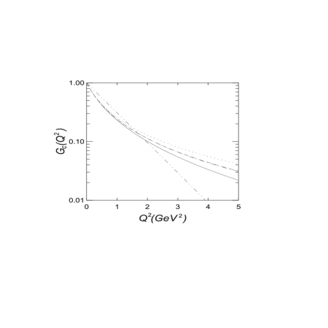
FIG. 1.: The results of the calculations of the $\rho$-meson charge form factor with different model wave functions. The values of the parameters are given in the Table I. The solid line represents the relativistic calculation with the wave function (84), the dashed line – with (85) for $n=$ 3, dash–dot–line – with (86), dotted line – with (85) for $n=$ 2, dot–dot–dash-line – the non-relativistic calculation with (84)

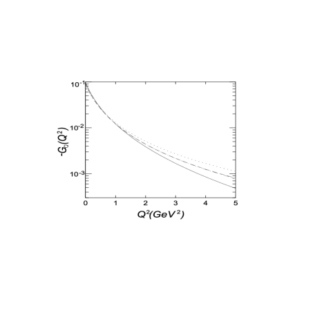
FIG. 2.: The results of the calculations of the $\rho$-meson quadrupole form factor with different model wave functions, legend as in Fig.1

FIG. 3.: The results of the calculations of the $\rho$-meson magnetic form factor with different model wave functions, legend as in Fig.1

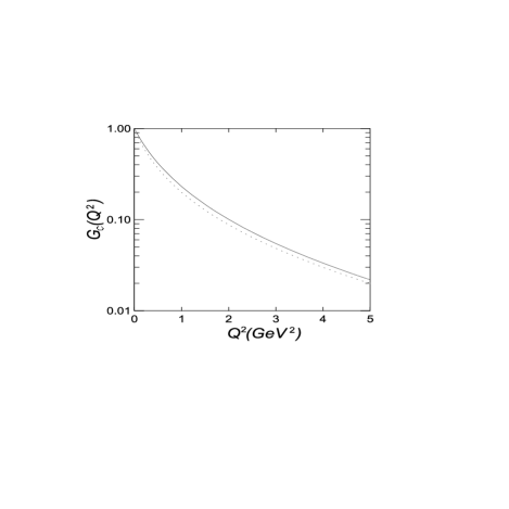
FIG. 4.: The contribution of the relativistic spin rotation effect. The results of the relativistic calculation of the $\rho$-meson charge form factor with the wave function (84) using the same parameters as in Fig.1. Solid line represents the relativistic calculation with spin rotation, dotted line – the relativistic calculation without spin rotation.

The spin rotation contribution to the magnetic moment in our calculations is 11%–12% and is negative, too. The total relativistic corrections to MSR in our approach are positive and enlarge the non-relativistic value essentially – almost twice in the case of the model (84) and for 70% – 80% for the models (85), (86).

The total relativistic corrections for the magnetic moment as compared to the non-relativistic result (see Eq. (95)) are negative and have the value of 21%–22%. Let us note, that in the light–front dynamics approach [15] a different result was obtained: the positive relativistic correction of the value of 10% to the magnetic moment.

Let us note especially that in our calculation of the $\rho$ – meson quadrupole moment no ambiguities connected with rotation symmetry arises – in contrast with the light–front dynamic calculations [14, 15].

The results of calculations for the $\rho$ – meson electromagnetic form factors are represented in Fig.1–3.

Let us note that our charge form factor has no dip in contrast with the results of the papers [14, 15]. This principal difference is probably due to the effects of rotation symmetry breaking in Refs. [14, 15]. The relativistic corrections in our approach diminish essentially the rate of the decreasing of the charge and magnetic form factors at large values of momentum transfer. We demonstrate in the figures the case of the model (84) with the exponential decreasing of the nonrelativistic form factors with the increasing $Q^{2}$. The nonrelativistic quadrupole form factor is zero in the absence of the $D$–state in the two–particle system.

In Fig.4 the contribution of Wigner rotation of quark spins to the $\rho$ – meson charge form factor is shown. This contribution depends weakly on the momentum transfer in the range from 1 to 5 GeV² and its value is approximately 10%. In our calculation the sign of this contribution differs from that obtained in the light–front dynamics approach [14]. Let us note that similar difference takes place in the case of pion electromagnetic structure, too (see calculations in Ref. [25] and Ref. [34]).

VII Conclusion

The method of construction of the electromagnetic current matrix elements for the relativistic two–particle composite systems with nonzero total angular momentum is developed in the frame of the instant form of RHD.

The method makes use of the Wigner–Eckart theorem on the Poincaré group. It enables one to extract from the matrix elements the reduced matrix elements – invariant form factors – which in the case of composite systems are generalized functions.

The obtained current operator matrix elements satisfy the Lorentz–covariance condition and the conservation law.

The modified impulse approximation — with the physical content of the relativistic impulse approximation — is formulated in terms of reduced matrix elements. MIA conserves Lorentz covariance of electromagnetic current and the current conservation law.

The developed formalism is used to obtain a reasonable description of the static moments and the electromagnetic form factors of $\rho$ meson. A number of relativistic effects are obtained, for example, the nonzero quadrupole moment (in the case of $S$ state) due to the relativistic Wigner spin rotation.

So, in conclusion, it is shown that the instant form of RHD can be used to obtain an adequate description of the electroweak properties of composite systems with nonzero total angular momentum.

REFERENCES

• [1] A.F. Krutov and V.E. Troitsky, Phys.Rev.C 65, 045501 (2002).
• [2] B.D. Keister and W. Polyzou, Adv. Nucl. Phys. 20, 225 (1991).
• [3] A.A. Cheshkov and Yu.M. Shirokov, Zh. Eksp. Teor. Fiz. 44, 1982 (1963).
• [4] V.E. Troitsky and Yu.M Shirokov, Teor.Math.Fiz. 1, 213 (1969).
• [5] V.P. Kozhevnikov, V.E. Troitsky, S.V. Trubnikov, and Yu.M. Shirokov, Teor. Mat. Fiz. 10, 47 (1972).
• [6] F.M. Lev, Ann. Phys. (N.Y.) 237, 355 (1995).
• [7] F. Gross and D.O. Riska, Phys. Rev. C 36, 1928 (1987); H. Ito, W.W. Buck, and F. Gross, ibid. 43, 2483 (1991); F. Gross and H. Henning, Nucl. Phys. A537, 344 (1992); F. Coester and D.O. Riska, Ann. Phys. (N.Y.) 234, 141 (1994).
• [8] P.L. Chung, F. Coester, B.D. Keister, and W.N. Polyzou, Phys. Rev. C 37, 2000 (1988).
• [9] V.A. Karmanov and A.V. Smirnov, Nucl.Phys. A546, 691 (1992); J. Carbonell, B. Desplanques, V.A. Karmanov, and J.–F. Mathjiot, Phys. Rep. 300, 215 (1998).
• [10] J.W. Van Orden, N. Devine, and F. Gross, Phys. Rev. Lett. 75, 4369 (1995).
• [11] F.M. Lev, E. Pace, and G. Salmé, Nucl. Phys. A641, 229 (1998).
• [12] J.P.B.C. de Melo, J.H.O. Sales, T. Frederico, and P.U. Sauer, Nucl. Phys. A631, 574 (1998).
• [13] W.H. Klink, Phys. Rev. C 58, 3587 (1998).
• [14] B.D. Keister, Phys. Rev.D 49, 1500 (1994).
• [15] F. Cardarelli, I.L. Grach, I.M. Narodetskii, G. Salmé , and S. Simula, Phys. Lett. B 349, 393 (1995).
• [16] I.L. Grach and L.A. Kondratyuk, Yad. Fiz. 39, 316 (1984)[Sov. J. Nucl. Phys. 39, 198 (1984)].
• [17] A.F. Krutov and V.E. Troitsky (to be published).
• [18] V.M. Dubovik and V.V. Tugushev, Phys. Rep. 187, 145 (1990).
• [19] Yu.M. Shirokov, Zh. Eksp. Teor. Fiz. 21, 748 (1951).
• [20] Yu.V. Novozhilov, Introduction to Elementary Particle Theory (Oxford University Press, New York, 1975).
• [21] A.A. Cheshkov, Zh. Eksp. Teor. Fiz. 50, 144 (1966).
• [22] E.V. Balandina and N.P. Yudin, Vestn. Mosk. Univ., Ser. 3: Fiz., Astron. 36, 14 (1995).
• [23] N.N. Bogoliubov, A.A. Logunov, A.I. Oksak, and I.T. Todorov, General Principles of Quantum Field Theory (Kluwer Academic, Dodrecht, 1990).
• [24] R.G. Arnold, C.E. Carlson, and F. Gross, Phys. Rev. C 21, 1426 (1980).
• [25] P.L. Chung, F. Coester, and W.N. Polyzou, Phys. Lett. B 205, 545 (1988).
• [26] M.V. Terentyev, Yad. Fiz. 24, 207 (1976); I.G. Aznauryan and N.L. Ter-Isaakyan, Yad. Fiz 31, 1680 (1980); W. Jaus, Phys. Rev. D 44, 2851 (1991); J. Carbonell and V.A. Karmanov, Eur. Phys. J. A 6, 9 (1999); F.M. Lev, E. Pace, and G. Salmé, Phys. Rev. C 62, 064004 (2000).
• [27] F. Schlumpf, Phys.Rev. D 50, 6895 (1994).
• [28] A.F. Krutov and V.E. Troitsky, J. Phys. G 19, L127 (1993), E.V. Balandina, A.F. Krutov, and V.E. Troitsky, J. Phys. G 22, 1585 (1996); A.F. Krutov, Yad. Fiz. 60, 1442 (1997)[Phys. At. Nucl. 60, 1305 (1997)]; E.V. Balandina, A.F. Krutov, V.E. Troitsky, and O.I. Shro, Yad. Fiz. 63, 301 (2000)[Phys. At. Nucl. 63, 244 (2000)].
• [29] J. Charles, A. Le Yaouanc, L. Oliver, O. Pène, and J.-C. Raynal, Phys. Lett. B 451, 187 (1999).
• [30] T.W. Allen and W.H. Klink, Phys. Rev. C 58, 3670 (1998); V.V. Andreev, Vestsi Nats. Akad. Navuk Belarusi, Ser. Fiz.-Mat. Navuk 2, 93 (2000); T.W. Allen, W.H. Klink, and W.N. Polyzou, Phys. Rev. C 63, 034002 (2001).
• [31] H. Tezuka, J. Phys. A 24, 5267 (1991).
• [32] F. Cardarelli, I.L. Grach, I.M. Narodetskii, E. Pace, G. Salmé, and S. Simula, Phys. Rev. D 53, 6682 (1996).
• [33] A.F. Krutov and V.E. Troitsky, Teor. Mat. Fiz. 116, 215 (1998)[Theor. Math. Phys. 116, 907 (1998)].
• [34] A.F. Krutov and V.E. Troitsky, J. High Energy Phys. 10, 028 (1999).
• [35] V.A. Matveev, R.M. Muradyan, and A.N. Tavkhelidze, Lett. Nuovo Cim. 7, 719 (1973), 15, 907 (1973); S. Brodsky and G. Farrar, Phys. Rev. Lett. 31, 1153 (1973).
• [36] A.F. Krutov and V.E. Troitsky, Eur. Phys. J. C 20, 71 (2001).
• [37] S.B. Gerasimov, JINR Report No. E2–89–837, Dubna, 1989; Phys.Lett. B 357, 666 (1995).
• [38] U. Vogl, M. Lutz, S. Klimt, and W. Weise, Nucl. Phys. A516, 469 (1990); B. Povh and J. Hüfner, Phys. Lett. B 245, 653 (1990); S.M. Troshin and N.E. Tyurin, Phys. Rev. D 49, 4427 (1994).
• [39] W. Lucha, F.F. Schöberl, and D. Gromes, Phys. Rep., 200, 127 (1991).
• [40] S.R. Amendolia et al., Phys. Lett. B 146, 116 (1984).
• [41] A. Abele et al., Phys. Lett. B 469, 270 (1999).
• [42] G.E. Brown and A.D. Jackson, The Nucleon–Nucleon Interaction (North–Holland, Amsterdam, 1976).
Appendix 1
The charge form factor for free two–particle system:
$$g_{0C}(s,Q^{2},s^{\prime})=\frac{1}{3}\,R(s,Q^{2},s^{\prime})\,Q^{2}\,$$
$$\times\left\{(s+s^{\prime}+Q^{2})\left[G^{u}_{E}(Q^{2})+G^{\bar{d}}_{E}(Q^{2})\right]\,\right.$$
$$\times\left[2\,\cos(\omega_{1}-\omega_{2})+\cos(\omega_{1}+\omega_{2})\right]$$
$$-\,\frac{1}{M}\xi(s,Q^{2},s^{\prime})\left[G^{u}_{M}(Q^{2})+G^{\bar{d}}_{M}(Q^{2})\right]\,$$
$$\left.\times\left[2\,\sin(\omega_{1}-\omega_{2})-\sin(\omega_{1}+\omega_{2})\right]\right\}\;,$$ (A1)𝐴1
The quadrupole form factor for free two–particle system:
$$g_{0Q}(s,Q^{2},s^{\prime})=\frac{1}{2}\,R(s,Q^{2},s^{\prime})\,Q^{2}\,$$
$$\times\left\{(s+s^{\prime}+Q^{2})\left[G^{u}_{E}(Q^{2})+G^{\bar{d}}_{E}(Q^{2})\right]\,\right.$$
$$\times\left[\cos(\omega_{1}-\omega_{2})-\cos(\omega_{1}+\omega_{2})\right]$$
$$-\,\frac{1}{M}\xi(s,Q^{2},s^{\prime})\left[G^{u}_{M}(Q^{2})+G^{\bar{d}}_{M}(Q^{2})\right]\,$$
$$\left.\times\left[\sin(\omega_{1}-\omega_{2})+\sin(\omega_{1}+\omega_{2})\right]\right\}\;,$$ (A2)𝐴2
The magnetic form factor for free two–particle system:
$$g_{0M}(s,Q^{2},s^{\prime})=-\,{2}\,R(s,Q^{2},s^{\prime})\,$$
$$\times\left\{\xi(s,Q^{2},s^{\prime})\left[G^{u}_{E}(Q^{2})+G^{\bar{d}}_{E}(Q^{2})\right]\,\sin(\omega_{1}-\omega_{2})\right.$$
$$+\frac{1}{4\,M}\left[G^{u}_{M}(Q^{2})+G^{\bar{d}}_{M}(Q^{2})\right]\,\left[(s+s^{\prime}+Q^{2})\,Q^{2}\,\right.$$
$$\times\left(\frac{3}{2}\,\cos(\omega_{1}-\omega_{2})+\frac{1}{2}\cos(\omega_{1}+\omega_{2})\right)$$
$$-\frac{1}{4}\xi(s,Q^{2},s^{\prime})$$
$$\times\left[\frac{(\sqrt{s^{\prime}}+2\,M)(s-s^{\prime}+Q^{2})+(s^{\prime}-s+Q^{2})\sqrt{s^{\prime}}}{\sqrt{s^{\prime}}(\sqrt{s^{\prime}}+2\,M)}\right.$$
$$\left.+\frac{(\sqrt{s}+2\,M)(s^{\prime}-s+Q^{2})+(s-s^{\prime}+Q^{2})\sqrt{s}}{\sqrt{s}(\sqrt{s}+2\,M)}\right]$$
$$\times\left[\sin(\omega_{1}-\omega_{2})-\sin(\omega_{1}+\omega_{2})\right]$$
$$-\frac{1}{2}\xi^{2}(s,Q^{2},s^{\prime})\left[\frac{1}{\sqrt{s^{\prime}}(\sqrt{s^{\prime}}+2\,M)}+\frac{1}{\sqrt{s}(\sqrt{s}+2\,M)}\right]$$
$$\left.\left.\times\left[\cos(\omega_{1}-\omega_{2})+\cos(\omega_{1}+\omega_{2})\right]\right]\right\}\;.$$ (A3)𝐴3
Here
$$R(s,Q^{2},s^{\prime})=\frac{(s+s^{\prime}+Q^{2})}{2\sqrt{(s-4M^{2})(s^{\prime}-4M^{2})}}\,$$
$$\times\frac{\vartheta(s,Q^{2},s^{\prime})}{{[\lambda(s,-Q^{2},s^{\prime})]}^{3/2}}\frac{1}{\sqrt{1+Q^{2}/4M^{2}}}\;,$$
$$\xi(s,Q^{2},s^{\prime})=\sqrt{ss^{\prime}Q^{2}-M^{2}\lambda(s,-Q^{2},s^{\prime})}\;,$$
$\omega_{1}$ $\omega_{2}$ – the Wigner rotation parameters:
$$\omega_{1}=\arctan\frac{\xi(s,Q^{2},s^{\prime})}{M\left[(\sqrt{s}+\sqrt{s^{\prime}})^{2}+Q^{2}\right]+\sqrt{ss^{\prime}}(\sqrt{s}+\sqrt{s^{\prime}})}\;,$$
$$\omega_{2}=\arctan\frac{\alpha(s,s^{\prime})\xi(s,Q^{2},s^{\prime})}{M(s+s^{\prime}+Q^{2})\alpha(s,s^{\prime})+\sqrt{ss^{\prime}}(4M^{2}+Q^{2})}\;,$$
here $\alpha(s,s^{\prime})=2M+\sqrt{s}+\sqrt{s^{\prime}}$, $\vartheta(s,Q^{2},s^{\prime})=\theta(s^{\prime}-s_{1})-\theta(s^{\prime}-s_{2})$, $\theta$ - the step–function.
$$s_{1,2}=2M^{2}+\frac{1}{2M^{2}}(2M^{2}+Q^{2})(s-2M^{2})$$
$$\mp\frac{1}{2M^{2}}\sqrt{Q^{2}(Q^{2}+4M^{2})s(s-4M^{2})}\;.$$
$M$ – the mass of $u$– and $\bar{d}$ quarks. The functions $s_{1,2}(s,Q^{2})$ give the kinematically available region in the plane $(s,s^{\prime})$. $G^{u,\bar{d}}_{E,M}(Q^{2})$– Sachs form factors of $u$– and $\bar{d}$ quarks.