The two-gluon components of the $\eta$ and $\eta^{\prime}$ mesons to leading-twist accuracy

Abstract

We critically reexamine the formalism for treating the leading-twist contributions from the two-gluon Fock components occurring in hard processes that involve $\eta$ and $\eta^{\prime}$ mesons and establish a consistent set of conventions for the definition of the gluon distribution amplitude, the anomalous dimensions as well as the projector of a two-gluon state onto an $\eta$ or $\eta^{\prime}$ state. We calculate the $\eta$, $\eta^{\prime}$–photon transition form factor to order $\alpha_{s}$ and show the cancellation of the collinear and UV singularities explicitly. An estimate of the lowest Gegenbauer coefficients of the gluon and quark distribution amplitudes is obtained from a fit to the $\eta$, $\eta^{\prime}$–photon transition form factor data. In order to elucidate the role of the two-gluon Fock component further, we analyze electroproduction of $\eta,\eta^{\prime}$ mesons and the $g^{*}g^{*}\eta(\eta^{\prime})$ vertex.

I Introduction

The description of hard exclusive processes involving light mesons is based on the factorization of the short- and long-distance dynamics sHSA ; LepageB80 . The former is represented by process-dependent, perturbatively calculable parton-level subprocess amplitudes, in which the mesons are replaced by their valence Fock components, while the latter is described by process-independent meson distribution amplitudes. This work is focused on hard reactions involving $\eta$ and $\eta^{\prime}$ mesons. These particles as other flavor neutral mesons possess SU(3)_F singlet and octet valence Fock components and, additionally, two-gluon ones; to all three of them correspond distribution amplitudes. This feature leads, on the one hand, to the well-known flavor mixing which, for the $\eta-\eta^{\prime}$ system, has been extensively studied (for a recent review, see Feldmann99 ) and, on the other hand, as a further complication, to mixing of the singlet and gluon distribution amplitudes under evolution. On the strength of more and better experimental data, the interest in hard reactions involving $\eta$ and $\eta^{\prime}$ mesons and, consequently, in the role of the two-gluon Fock component, has been renewed. Examples of such reactions are the meson-photon transition form factors, photo- and electroproduction of mesons or charmonium and $B$-meson decays.

Mixing of the singlet and gluon distribution amplitudes has been investigated in a number of papers Terentev81 –BelitskyM98 . Apart from differences in the notation and occasional misprints, different prefactors appear in the evolution kernels and in the expressions for the anomalous dimensions. Often the full set of conventions for kernels, anomalous dimensions, the gluon distribution amplitude and the gluon-meson projector is not provided and/or it is not easy to extract. This makes the comparison of the various theoretical results and their applications difficult. We therefore reexamine the treatment of the gluon distribution amplitude and its mixing with the singlet one. This analysis is performed in the context of the $\eta\gamma$ and $\eta^{\prime}\gamma$ transition form factors. Applying the methods proposed in MelicNP01 , we calculate them to leading-twist accuracy and include next-to-leading order (NLO) perturbative QCD corrections. Our investigation enables us to introduce and to test the conventions for the ingredients of a leading-twist calculation for any hard process that involves $\eta$ or $\eta^{\prime}$ mesons. The most crucial test of the consistency of our set of conventions is the cancellation of the collinear singularities present in the parton-subprocess amplitude with the ultraviolet (UV) singularities appearing in the unrenormalized distribution amplitudes. Our analysis permits a critical appraisal of the relevant literature Terentev81 –BelitskyM98 .

In analogy with the analysis of the $\pi\gamma$ transition form factor DiehlKV01 , we use our leading-twist NLO results for the transition form factors to extract information on the $\eta$ and $\eta^{\prime}$ distribution amplitudes from fits to the experimental data CLEO97 ; L398 . In order to make contact with experiment we have to adopt an appropriate $\eta-\eta^{\prime}$ mixing scheme. We assume particle independence of the distribution amplitudes reducing so their number to three. Consequently, flavor mixing is solely encoded in the decay constants for which we use the values determined in FeldmannKS98 .

Our set of conventions, as abstracted from the calculation of the transition form factor, is then appropriate for general use in leading-twist calculations of hard exclusive reactions involving $\eta$ and $\eta^{\prime}$ mesons. We briefly discuss a few of them, namely, electroproduction of the $\eta$ and $\eta^{\prime}$ mesons and the vertex $g^{*}g^{*}\eta(\eta^{\prime})$, in order to learn more about the importance of the gluon distribution amplitudes. In contrast to the transition form factors, the two-gluon Fock components contribute in these reactions to the same order of the strong coupling constant, $\alpha_{s}$, as the quark-antiquark ones. The two-gluon components also contribute to the decays $\chi_{cJ}\to\eta\eta,\eta^{\prime}\eta^{\prime}$. The analysis of these decays is however intricate since the next higher Fock state of the $\chi_{cJ}$, ${c}\overline{c}g$ contributes to the same inverse power of the relevant hard scale, the charm quark mass, as the ${c}\overline{c}$ state and has to be taken into account in a consistent analysis BolzKS96 . We therefore refrain from analysing these decays here.

The plan of the paper is the following: The calculation of the meson-photon transition form factors is presented in Sec. II. In Sec. III we discuss $\eta-\eta^{\prime}$ flavor mixing while Sec. IV is devoted to a comparison with experiment and the extraction of the size of the lowest Gegenbauer coefficients of the quark and gluon distribution amplitudes. In Sec. V we investigate the role of the gluon distribution amplitude in other hard reactions. The summary is presented in Sec. VI. The paper ends with three appendices in which we compile the definitions of quark and gluon distribution amplitudes (App. A), calculational details for the transition form factors (App. B) and some properties of the evolution kernels (App. C).

II The $P\gamma$ transition form-factor

II.1 The flavor-singlet case

As the valence Fock components of the pseudoscalar mesons $P=\eta,\eta^{\prime}$, we choose SU(3)_F singlet and octet combinations of quark-antiquark states

$$|q\overline{q}_{1}\rangle = |({u}\overline{u}+{d}\overline{d}+{s}\overline{s})/\sqrt{3}\rangle\,,$$

$$|q\overline{q}_{8}\rangle = |({u}\overline{u}+{d}\overline{d}-2{s}\overline{s})/\sqrt{6}\rangle\,,$$ (1)

and the two-gluon state $|gg\rangle$ which also possess flavor-singlet quantum numbers and contributes to leading twist. The corresponding distribution amplitudes are denoted by $\phi_{P1,8,g}$; their formal definitions are given in App. A. We emphasize that here, in this section, we do not make use of a flavor mixing scheme since the theoretical treatment of the transition form factors is independent of it. As usual the decay constants, defined by the vacuum-meson matrix elements of flavor-singlet or octet weak axial vector currents ($i=1,8$)

$$\langle 0|J^{i}_{\mu 5}(0)|P(p)\rangle=if_{P}^{i}\,p_{\mu}\,,$$ (2)

or rather the factors $f_{P}^{i}/(2\sqrt{2N_{c}})$, are pulled out of the distribution amplitudes ($N_{c}$ being the number of colors). Hence, the quark distribution amplitudes are normalized to unity at any scale $\mu^{2}$

$$\int_{0}^{1}du\,\phi_{Pi}(u,\mu^{2})=1\,,$$ (3)

as follows from (2) and (89). From (LABEL:eq:melemg1u) one has

$$\int_{0}^{1}du\,\phi_{Pg}(u,\mu^{2})=0\,.$$ (4)

There is no natural way to normalize the gluon distribution amplitude. Since the flavor-singlet quark and gluon distribution amplitudes mix under evolution while the flavor-octet one evolves independently with the hard scale, it is convenient to pull out of the gluon distribution amplitude the same factor as for the flavor-singlet quark one.

As usual we parameterize the $\gamma^{*}(q_{1},\mu)\,\gamma(q_{2},\nu)\rightarrow P(p)$ vertex as

$$\Gamma^{\mu}=i\,e^{2}\;F_{P\gamma}(Q^{2})\;\varepsilon^{\mu\nu\alpha\beta}\;\epsilon_{\nu}(q_{2})\;q_{1\alpha}q_{2\beta}\,,$$ (5)

where $Q^{2}=-q_{1}^{2}\geq 0$ is the momentum transfer, and $F_{P\gamma}(Q^{2})$ denotes the $P\gamma$ transition form factor. It can be represented as a sum of the flavor-octet and the flavor-singlet contributions

$$F_{P\gamma}(Q^{2})=F_{P\gamma}^{\,8}(Q^{2})+F_{P\gamma}^{\,1}(Q^{2})\,,$$ (6)

where the latter one includes the quark and the gluon part. The leading-twist singlet contribution to order $\alpha_{s}$ is unknown, while the octet contribution is well-known to this order, one only has to adapt the result for the $\pi\gamma$ transitions piontff suitably. We therefore perform a detailed analysis of the singlet contribution along the lines of the flavor-octet analysis presented in MelicNP01 .

For large momentum transfer $Q^{2}$, the flavor-singlet contribution to the transition form factor can be represented as a convolution (see Fig. 1 for a lowest order Feynman diagram)

$$F_{P\gamma}^{\,1}(Q^{2})=\frac{f_{P}^{1}}{2\sqrt{2N_{c}}}\;T^{\dagger}(u,Q^{2})\,\otimes\,\phi_{P}^{ur}(u)\,,$$ (7)

where the symbol $\otimes$ represents the usual convolution $A(z)\otimes B(z)=\int_{0}^{1}dzA(z)B(z)\,.$ We employ a two-component vector notation

$$\phi_{P}^{ur}(u)\equiv\left(\begin{array}[c]{c}\phi^{ur}_{Pq}(u)\\[1.99997pt] \phi^{ur}_{Pg}(u)\end{array}\right)\,,\qquad T(u,Q^{2})\equiv\left(\begin{array}[c]{c}T_{q\overline{q}}(u,Q^{2})\\[1.99997pt] T_{gg}(u,Q^{2})\end{array}\right)\,,$$ (8)

and switch to the more generic notation $\phi_{Pq}\equiv\phi_{P1}$. The unrenormalized quark and gluon distribution amplitudes $\phi^{ur}_{Pq}$ and $\phi^{ur}_{Pg}$ are defined in Eqs. (84) and (85). The parton-level subprocesses amplitudes for $\gamma^{*}\gamma\rightarrow q\overline{q}$, and $\gamma^{*}\gamma\rightarrow gg$ are denoted by $T_{q\overline{q}}$ and $T_{gg}$, respectively; the Lorentz structure is factorized out as in (5).

Figure 1: Lowest order Feynman diagram for the $\gamma^{*}\gamma\to P$ transition. A second diagram is obtained by interchanging the photon vertices.

The distribution amplitudes $\phi^{ur}_{Pq}$ and $\phi^{ur}_{Pg}$ require renormalization which introduces mixing of the composite operators $\bar{\Psi}(-z)\,\gamma^{+}\gamma_{5}\,\Omega\,\Psi(z)$ and $G^{+\alpha}(-z)\,\Omega\,\widetilde{G}^{\>\>\>+}_{\alpha}(z)$. The unrenormalized distribution amplitude $\phi^{ur}_{P}$ is related to the renormalized one, $\phi_{P}$, by

$$\phi^{ur}_{P}(u)=Z(u,x,\mu^{2}_{F})\otimes\phi_{P}(x,\mu^{2}_{F})\,,$$ (9)

where the UV-divergent renormalization matrix takes the form

$$Z\equiv\left(\begin{array}[]{cc}Z_{qq}&Z_{qg}\\[1.99997pt] Z_{gq}&Z_{gg}\end{array}\right)\,.$$ (10)

Here, $\mu^{2}_{F}$ represents the scale at which the singularities and, hence, soft and hard physics, are factorized. Owing to the fact that quarks and gluons are taken to be massless and onshell, $T_{q\overline{q}}$ and $T_{gg}$, calculated beyond leading order, contain collinear singularities. The validity of factorization into hard and soft physics, as expressed in (7), requires the cancellation of these singularities with the UV ones from the renormalization of the distribution amplitudes. Hence, the hard scattering amplitude defined by

$$T_{H}^{\dagger}(x,Q^{2},\mu^{2}_{F})=T^{\dagger}(u,Q^{2})\otimes Z(u,x,\mu^{2}_{F})\,,$$ (11)

must be finite. Below we explicitly show this cancellation to NLO. Provided the cancellation of the singularities holds, the transition form factor can be expressed in terms of finite hard scattering and distribution amplitudes

$$F_{P\gamma}^{\,1}(Q^{2})=\frac{f^{1}_{P}}{2\sqrt{2N_{c}}}\;T_{H}(x,Q^{2},\mu^{2}_{F})^{\dagger}\,\otimes\phi_{P}(x,\mu^{2}_{F})\,.$$ (12)

II.2 The NLO hard-scattering amplitude

We now proceed to the NLO calculation. The renormalization matrix $Z$, can be shown to have the following form

$$Z=\mathbf{1}+\frac{\alpha_{s}(\mu^{2}_{F})}{4\pi}\,\frac{1}{\epsilon}\,V^{(1)}+{\cal O}(\alpha_{s}^{2})\,,$$ (13)

if dimensional regularization ($D=4-2\epsilon$) is employed. Here $\mathbf{1}$ denotes the unit $2\times 2$ matrix (with diagonal elements $\delta(x-u)$), and the coefficient $V^{(1)}=V^{(1)}(x,u)$ is a matrix

$$V^{(1)}\equiv\left(\begin{array}[]{cc}V_{qq}&V_{qg}\\[5.69046pt] V_{gq}&V_{gg}\end{array}\right)\,.$$ (14)

The amplitudes $T_{q\bar{q}}$ and $T_{gg}$ have well-defined expansions in $\alpha_{s}$, and after coupling-constant renormalization, which introduces the renormalization scale $\mu^{2}_{R}$, they read

$$T_{q\bar{q}}(u) = \frac{N_{q\bar{q}}}{Q^{2}}\left[T_{q\bar{q}}^{(0)}(u)\right.$$

$$\left.+\frac{\alpha_{s}(\mu^{2}_{R})}{4\pi}\,C_{F}\,\left(\frac{\mu^{2}_{R}}{Q^{2}}\right)^{\epsilon}T_{q\bar{q}}^{(1)}(u)+{\cal O}(\alpha_{s}^{2})\right]\,,$$

$$T_{gg}(u) = \frac{N_{gg}}{Q^{2}}\left[\frac{\alpha_{s}(\mu^{2}_{R})}{4\pi}\left(\frac{\mu^{2}_{R}}{Q^{2}}\right)^{\epsilon}T_{gg}^{(1)}(u)+{\cal O}(\alpha_{s}^{2})\right]\,.$$

The normalization factors $N_{q\overline{q}}$ and $N_{gg}$ in (LABEL:eq:expT) are given by

$$N_{q\bar{q}}=2\;\sqrt{2N_{c}}\;C_{1}\,,\qquad N_{gg}=\sqrt{n_{f}\,C_{F}}\,N_{q\overline{q}}\,,$$ (16)

where the flavor factor $C_{1}$ takes into account the quark content of the $q\overline{q}_{1}$ combination. It reads (see (81))

$${}C_{1}=\frac{e_{u}^{2}+e_{d}^{2}+e_{s}^{2}}{\sqrt{n_{f}}}\,.$$ (17)

The number of flavors in the $q\overline{q}_{1}$ is denoted by $n_{f}$ and $C_{F}=(N_{c}^{2}-1)/(2N_{c})$ is the usual color factor. $e_{a}$ is the charge of quark $a$ in units of the positron charge $e$.

Inserting (13) and (LABEL:eq:expT) into (11) and using (98), we obtain

$$T_{H,q\bar{q}} = \frac{N_{q\bar{q}}}{Q^{2}}\left\{T_{q\bar{q}}^{(0)}+\frac{\alpha_{s}(\mu^{2}_{R})}{4\pi}\left[C_{F}\,T_{q\bar{q}}^{(1)}\left(\frac{\mu^{2}_{R}}{Q^{2}}\right)^{\epsilon}\right.\right.$$

$$\left.\left.+\frac{1}{\epsilon}T_{q\bar{q}}^{(0)}\otimes V_{qq}\left(\frac{\mu^{2}_{R}}{\mu^{2}_{F}}\right)^{\epsilon}\,\right]+{\cal O}(\alpha_{s}^{2})\right\}\,,\;$$

$$T_{H,gg} = \frac{N_{gg}}{Q^{2}}\left\{\frac{\alpha_{s}(\mu^{2}_{R})}{4\pi}\left[T_{gg}^{(1)}\left(\frac{\mu^{2}_{R}}{Q^{2}}\right)^{\epsilon}\right.\right.$$

$$\left.\left.+\frac{N_{q\bar{q}}}{N_{gg}}\,\frac{1}{\epsilon}T_{q\bar{q}}^{(0)}\otimes V_{qg}\left(\frac{\mu^{2}_{R}}{\mu^{2}_{F}}\right)^{\epsilon}\,\right]+{\cal O}(\alpha_{s}^{2})\right\}.$$

Results for $T_{q\overline{q}}^{(0)}$, $T_{q\overline{q}}^{(1)}$, $T_{gg}^{(1)}$, and $V_{ij}$ and some details of their calculation are given in App. B. Using the results for $T^{(0)}_{q\overline{q}}$ and $V_{qq}$, it is easy to verify that

$$T^{(0)}_{q\overline{q}}(u)\,\otimes\,V_{qq}(u,x)=C_{F}\;{\cal A}_{col,q\bar{q}}^{(1)}(x)\,,$$ (19)

with ${\cal A}_{col,q\bar{q}}^{(1)}$ being given in (102). On the other hand, ${\cal A}_{col,q\bar{q}}^{(1)}$ is the residue of the $1/\epsilon$ pole in $T^{(1)}_{q\overline{q}}$, see (101). Hence, the collinear singularity present in $T_{q\overline{q}}^{(1)}$ is canceled by the UV singularity in $Z_{qq}$ and we arrive at a finite hard-scattering amplitude for the $\gamma^{*}\gamma\to q\overline{q}$ subprocess

$$T_{H,q\overline{q}}(x,Q^{2},\mu^{2}_{F})$$ (20)

$$= \frac{N_{q\overline{q}}}{Q^{2}}\left\{T_{H,q\overline{q}}^{(0)}(x)+\frac{\alpha_{s}(\mu^{2}_{R})}{4\pi}\,C_{F}\;T_{H,q\overline{q}}^{(1)}(x,Q^{2},\mu^{2}_{F})\right.$$

$$+{\cal O}(\alpha_{s}^{2})\Big{\}}\,,$$

where

$$T_{H,q\overline{q}}^{(0)}(x) = T_{q\overline{q}}^{(0)}(x)\,,$$

$$T_{H,q\bar{q}}^{(1)}(x,Q^{2},\mu^{2}_{F}) = -{\cal A}_{col,q\bar{q}}^{(1)}(x)\ln\frac{\mu^{2}_{F}}{Q^{2}}+{\cal A}_{q\bar{q}}^{(1)}(x)\,.$$

The quantities $T_{q\overline{q}}^{(0)}$, ${\cal A}_{col,q\bar{q}}^{(1)}$, and ${\cal A}_{q\bar{q}}^{(1)}$ are given in (101, 102).

Next, from (101) and (117), we obtain

$$T^{(0)}_{q\overline{q}}(u)\,\otimes\,V_{qg}(u,x)=\frac{N_{gg}}{N_{q\overline{q}}}\,{\cal A}_{col,gg}^{(1)}(x)\,,$$ (22)

with ${\cal A}_{col,gg}^{(1)}$ defined in (LABEL:eq:agg). Inserting this result into (LABEL:eq:expTH) and taking into account (104), we observe the cancellation of the collinear singularity present in $T_{gg}^{(1)}$ with the UV singularity of $Z_{qg}$, and we get the finite hard-scattering amplitude for the $\gamma^{*}\gamma\to gg$ subprocess

$$T_{H,gg}(x,Q^{2})=\frac{N_{gg}}{Q^{2}}\left[\frac{\alpha_{s}(\mu^{2}_{R})}{4\pi}T_{H,gg}^{(1)}(x,Q^{2},\mu^{2}_{F})+{\cal O}(\alpha_{s}^{2})\right]\,,$$ (23)

where $T_{H,gg}^{(1)}$ reads

$$T_{H,gg}^{(1)}(x,Q^{2},\mu^{2}_{F})=-{\cal A}_{col,gg}^{(1)}(x)\ln\frac{\mu^{2}_{F}}{Q^{2}}+{\cal A}_{gg}^{(1)}(x)\,.$$ (24)

The functions ${\cal A}_{col,gg}^{(1)}$ and ${\cal A}_{gg}^{(1)}$ are supplied in (LABEL:eq:agg).

II.3 Evolution of the flavor-singlet quark and gluon distribution amplitudes

We now turn to the discussion of the distribution amplitude $\phi_{P}$ and its evolution. The matrix $Z$ is related to the evolution of the distribution amplitude, and $V^{(1)}$ in (13) represents the kernel which governs the leading-order (LO) evolution of the flavor-singlet distribution amplitude. By differentiating (9) with respect to $\mu^{2}_{F}$ one obtains the evolution equation Terentev81 ; BaierG81

$$\mu^{2}_{F}\frac{\partial}{\partial\mu^{2}_{F}}\phi_{P}(x,\mu^{2}_{F})=V(x,u,\alpha_{s}(\mu^{2}_{F}))\,\otimes\,\phi_{P}(u,\mu^{2}_{F})\,,$$ (25)

where the evolution kernel $V$ reads

$$V=-Z^{-1}\,\otimes\,\left(\mu^{2}_{F}\frac{\partial}{\partial\mu^{2}_{F}}Z\right)\,.$$ (26)

We note in passing that the evolution equation would have a more complicated form if the factor $f_{P1}/(2\sqrt{2N_{c}})$ was not pulled out of the gluon distribution amplitude. Inserting (13) into (26), and using (99), one easily sees that

$$V=\frac{\alpha_{s}(\mu^{2}_{F})}{4\pi}\,V^{(1)}+{\cal O}(\alpha_{s}^{2})\,.$$ (27)

The results for the LO kernel $V^{(1)}$ are given in (109) and (117-124). The anomalous dimensions that control the evolution of the distribution amplitudes can be read off from the relations (127):

$$\gamma^{\,qq}_{n} = C_{F}\left[3+\frac{2}{(n+1)(n+2)}-4\sum_{i=1}^{n+1}\frac{1}{i}\right]\,,$$

$$\gamma^{\,qg}_{n} = \sqrt{n_{f}C_{F}}\;\ \frac{n(n+3)}{3(n+1)(n+2)}\qquad n\geq 2\,,$$

$$\gamma^{\,gq}_{n} = \sqrt{n_{f}C_{F}}\;\frac{12}{\phantom{3}(n+1)(n+2)}\qquad n\geq 2\,,$$

$$\gamma^{\,gg}_{n} = \beta_{0}+N_{c}\left[\frac{8}{(n+1)(n+2)}-4\sum_{i=1}^{n+1}\frac{1}{i}\right]\qquad n\geq 2\,.$$

To leading order in $\alpha_{s}$ the evolution equation (25) can be solved by diagonalizing the kernel $V$ or rather the matrix of the anomalous dimensions. The eigenfunctions can be expanded upon the Gegenbauer polynomials $C_{n}^{m/2}$ with coefficients $B_{Pn}^{(\pm)}$ which evolve with the eigenvalues $\gamma_{n}^{(\pm)}$ of the matrix of the anomalous dimensions

$$\gamma^{\,(\pm)}_{n}=\frac{1}{2}\left[\gamma^{qq}_{n}+\gamma^{gg}_{n}\pm\sqrt{\left(\gamma^{qq}_{n}-\gamma^{gg}_{n}\right)^{2}+4\gamma^{qg}_{n}\gamma^{gq}_{n}}\right]\,.$$ (29)

The two components of the distribution amplitude $\phi_{P}$ possess the expansion

$$\phi_{Pq}(x,\mu^{2}_{F}) = 6x\,(1-x)\,\Big{[}1$$

$$+\sum_{n=2,4,\ldots}{\ B_{Pn}^{\,q}(\mu^{2}_{F})}\>C_{n}^{\,3/2}(2x-1)\Big{]}\,,$$

$$\phi_{Pg}(x,\mu^{2}_{F}) = x^{2}(1-x)^{2}$$

$$\times\sum_{n=2,4,\ldots}{B_{Pn}^{\,g}(\mu^{2}_{F})}\>C_{n-1}^{\,5/2}(2x-1)\,,$$

where only the terms for even $n$ occur as a consequence of (88). The expansion coefficients in (LABEL:eq:solphi) are related to those of the eigenfunctions by

$${B_{Pn}^{\,q}\,(\mu^{2}_{F})} = B_{Pn}^{(+)}(\mu_{0}^{2})\left(\frac{\alpha_{s}(\mu_{0}^{2})}{\alpha_{s}(\mu^{2}_{F})}\right)^{{\gamma^{\,(+)}_{n}}/{\beta_{0}}}$$

$$+\,{\rho_{n}^{\,(-)}}\,B_{Pn}^{(-)}\,(\mu_{0}^{2})\left(\frac{\alpha_{s}(\mu_{0}^{2})}{\alpha_{s}(\mu^{2}_{F})}\right)^{{\gamma^{\,(-)}_{n}}/{\beta_{0}}},$$

$${B_{Pn}^{\,g}\,(\mu^{2}_{F})} = {\rho_{n}^{\,(+)}}\,B_{Pn}^{(+)}\,(\mu_{0}^{2})\left(\frac{\alpha_{s}(\mu_{0}^{2})}{\alpha_{s}(\mu^{2}_{F})}\right)^{{\gamma^{\,(+)}_{n}}/{\beta_{0}}}$$ (31)

$$+\,B_{Pn}^{(-)}\,(\mu_{0}^{2})\left(\frac{\alpha_{s}(\mu_{0}^{2})}{\alpha_{s}(\mu^{2}_{F})}\right)^{{\gamma^{\,(-)}_{n}}/{\beta_{0}}}.$$

The coefficients $B_{Pn}^{(\pm)}\,(\mu_{0}^{2})$ respective $B_{Pn}^{\,q,g}\,(\mu_{0}^{2})$, where $\mu_{0}^{2}$ is the initial scale of the evolution, represent the non-perturbative input to a calculation of the transition form factors and are, at present, not calculable with a sufficient degree of accuracy. The parameters $\rho_{n}^{\,(\pm)}$ read

$$\rho_{n}^{\,(+)}=6\;\frac{\gamma^{\,gq}_{n}}{\gamma^{\,(+)}_{n}-\gamma^{\,gg}_{n}}\,,\qquad\rho_{n}^{\,(-)}=\frac{1}{6}\;\frac{\gamma^{\,qg}_{n}}{\gamma^{\,(-)}_{n}-\gamma^{\,qq}_{n}}\,.$$ (32)

We note that the anomalous dimensions satisfy the relation

$$\frac{\gamma^{\,qg}_{n}}{\gamma^{\,(\pm)}_{n}-\gamma^{\,qq}_{n}}=\frac{\gamma^{\,(\pm)}_{n}-\gamma^{\,gg}_{n}}{\gamma^{\,gq}_{n}}\,.$$ (33)

Comparison of (LABEL:eq:andim) and (29) reveals that $\gamma_{n}^{(+)}\approx\gamma^{qq}_{n}$ for all $n$ and $\gamma_{n}^{(+)}\to\gamma^{qq}_{n}$ for $n\to\infty$.

It is important to realize that any change of the definition of the gluon distribution amplitude (85) is accompanied by a corresponding change in the hard scattering amplitude. Suppose we change $\phi_{Pg}$ by a factor $\sigma$

$$\phi^{\,\sigma}_{Pg}=\sigma\,\phi_{Pg}\,.$$ (34)

Since any physical quantity, as for instance the transition form factor, must be independent of the choice of the convention, the projection (94) of $gg$ state onto a pseudoscalar meson state is to be modified by a factor $1/\sigma$, i.e.,

$${\cal P}^{g\,\sigma}_{\,\mu\nu}=\frac{1}{\sigma}\,{\cal P}^{g}_{\,\mu\nu}\,,$$ (35)

and the hard-scattering amplitude becomes altered accordingly. As an inspection of Eqs. (LABEL:eq:solphi)-(32) reveals, the change of the definition of the gluon distribution amplitude (34) has to be converted into a change of the off-diagonal anomalous dimensions and the Gegenbauer coefficients $B_{Pn}^{(\pm)}$ in order to leave the quark distribution amplitude as it is:

$$\gamma^{\,qg,\sigma}_{n}=\frac{1}{\sigma}\,\gamma^{\,qg}_{n}\,,\qquad\gamma^{\,gq,\sigma}_{n}=\sigma\,\gamma^{\,gq}_{n}\,,$$ (36)

and

$${B}^{(-)\,\sigma}_{Pn}\,(\mu_{0}^{2})=\sigma B^{(-)}_{Pn}\,(\mu_{0}^{2})\,,\qquad B^{(+)\,\sigma}_{Pn}\,(\mu_{0}^{2})=B^{(+)}_{Pn}\,(\mu_{0}^{2})\,,$$ (37)

implying

$$B^{\,g\,\sigma}_{Pn}\,(\mu^{2}_{F})=\sigma\,B^{\,g}_{Pn}\,(\mu^{2}_{F})\,,\qquad B^{\,q\,\sigma}_{Pn}\,(\mu^{2}_{F})=B^{\,q}_{Pn}\,(\mu^{2}_{F})\,.$$ (38)

We finally mention that, as can be easily seen from Eq. (34) and the evolution equation (25), along with the change of the anomalous dimensions (36) the kernels $V_{qg}$ and $V_{gq}$ become modified.

The results for the anomalous dimensions can also be understood in the operator language, i.e., by considering the impact of a change of the definition of the gluonic composite operator on the anomalous dimensions (for comments on the use of the operator product expansion, see, for instance, Refs. ShifmanV81 ; BaierG81 ). One finds that only the anomalous dimensions $\gamma^{\,qg}_{n}$ and $\gamma^{\,gq}_{n}$ become modified, while the diagonal ones and the product $\gamma^{\,qg}_{n}\,\gamma^{\,gq}_{n}$, and consequently the eigenvalues $\gamma_{n}^{(\pm)}$, remain unchanged. Redefinition of the gluonic composite operator implies a corresponding change of the gluon distribution amplitude.

We are now in the position to compare the results presented in this work with other calculations to be found in the literature. The entire set of conventions is not always easy to extract from the literature since often only certain aspects of the flavor-singlet system are discussed. For instance, in Ref. BlumleinGR97 only the evolution kernels are investigated, or in Ref. ShifmanV81 only the anomalous dimensions. Using results from such work in a calculation of a hard process necessitates the use of corresponding conventions for the other quantities. Care is also required if elsewhere determined numerical results for the Gegenbauer coefficients $B_{Pn}^{(-)}$ or $B_{Pn}^{g}$ are employed since, according to (37) and (38), they are convention dependent. For future reference, we systematize in Tab. 1 the important ingredients for the three conventions encountered in the literature. Our expressions for the kernels and the anomalous dimensions correspond to the ones obtained in Terentev81 (up to a typo in $V_{gg}$). In Refs. BelitskyM98etc ; BelitskyM98 the anomalous dimensions controlling the evolution of the forward and non-forward parton distribution were studied to NLO. Since the non-diagonal anomalous dimension for the odd parity case coincides with our ones MikhailovR , we observe that the convention $\sigma=\sqrt{C_{F}/n_{f}}$ is used in BelitskyM98etc ; BelitskyM98 . The only result we do not understand is the one presented in Ref. Ohrndorf81 : There is an extra factor of $1/2$ in $V_{gq}$ which changes the product of prefactors. Moreover, there are factors $1/3$ and $3$ apparently missing in $\gamma_{qg}$ and $\gamma_{gq}$. We note that occasionally the factor $[x(1-x)]^{-1}$ appearing in our projector (94) is absorbed into the gluon distribution amplitude Ohrndorf81 ; BaierG81 . This arrangement is accompanied by corresponding changes of the evolution kernels, see (125).

Table 1: List of common conventions for the anomalous dimensions and the $gg$ projector. Quoted are the prefactors of the non-diagonal anomalous dimensions (LABEL:eq:andim) and of the $gg$ projector (94) for various choices of $\sigma$ in (35, 36). We also list references where these conventions for the anomalous dimensions are used.

$\sigma$	$\gamma^{\,qg,\sigma}_{n}$	$\gamma^{\,gq,\sigma}_{n}$	${\cal P}^{g\sigma}_{\mu\nu}$	references
$1$	$\sqrt{n_{f}\,C_{F}}$	$\sqrt{n_{f}\,C_{F}}$	$1$	Terentev81
$\displaystyle\sqrt{\frac{n_{f}}{C_{F}}}$	$C_{F}$	$n_{f}$	$\displaystyle\sqrt{\frac{C_{F}}{n_{f}}}$	ShifmanV81 ; BaierG81
$\displaystyle\sqrt{\frac{C_{F}}{n_{f}}}$	$n_{f}$	$C_{F}$	$\displaystyle\sqrt{\frac{n_{f}}{C_{F}}}$	BlumleinGR97 ; BelitskyM98

Although, from the point of view of derivation, the conventions which lead to (LABEL:eq:andim) and (94) seem to be the most natural ones, it is perhaps more expedient to use the same conventions for the anomalous dimensions as for polarized deep inelastic lepton-proton scattering AhmedR76 , which correspond to

$$\sigma=\sqrt{\frac{n_{f}}{C_{F}}}\,.$$ (39)

The corresponding set of conventions will be used in the rest of the paper. The non-diagonal anomalous dimensions then read

$$\gamma^{\,qg}_{n} \longrightarrow C_{F}\;\ \frac{n(n+3)}{3(n+1)(n+2)}\qquad n\geq 2\,,$$

$$\gamma^{\,gq}_{n} \longrightarrow n_{f}\;\frac{12}{\phantom{3}(n+1)(n+2)}\qquad n\geq 2\,,$$ (40)

and the gluonic projector

$${\cal P}^{g}_{\mu\nu,ab}\longrightarrow\,\frac{i}{2}\;\sqrt{\frac{C_{F}}{n_{f}}}\;\frac{\delta_{ab}}{\sqrt{N_{c}^{2}-1}}\;\frac{\varepsilon_{\perp\mu\nu}}{u(1-u)}\,.$$ (41)

Along with these definitions, Eqs. (LABEL:eq:solphi)-(32) have to be used.

To the order we are working, the NLO evolution of the quark distribution amplitudes should in principle be included (the convolution of the NLO term for $\phi_{Pg}$ with $T_{H,gg}$ contributes to order $\alpha_{s}^{2}$). To NLO accuracy the Gegenbauer polynomials $C_{n}^{3/2}$ are no longer eigenfunctions of the evolution kernel, so that their coefficients $B_{Pn}^{i}$ do not evolve independently BelitskyM98 ; Muller95 . In analogy with the pion case KrollR96 , the impact of the NLO evolution on the transition form factors is expected to be small compared with the NLO corrections to the subprocess amplitudes. Therefore we refrain from considering NLO evolution.

II.4 The NLO result for the transition form factor

To end this section we quote our final result for the flavor-singlet contribution to the $P\gamma$ transition form factor to leading-twist accuracy and NLO in $\alpha_{s}$. The result, obtained by inserting (20) and (23) (multiplied by $\sigma^{-1}=\sqrt{C_{F}/n_{f}}$ according to the new normalization of the gluonic projector) into (12), is

$$F_{P\gamma}^{\,1}(Q^{2})$$

$$= \frac{f^{1}_{P}\,C_{1}}{Q^{2}}\;\left\{T_{H,q\bar{q}}^{(0)}(x)\otimes\phi_{Pq}(x,\mu^{2}_{F})\right.$$

$$\left.+\frac{\alpha_{s}(\mu^{2}_{R})}{4\pi}\,C_{F}\,\left[\;T_{H,q\overline{q}}^{(1)}(x,Q^{2},\mu^{2}_{F})\otimes\phi_{Pq}(x,\mu^{2}_{F})\right.\right.$$

$$\left.\left.\hskip 62.59596pt+T_{H,gg}^{(1)}(x,Q^{2},\mu^{2}_{F})\otimes\phi_{Pg}(x,\mu^{2}_{F})\right]\,\right\}\,.$$

A subtlety has to be mentioned. The singlet decay constant, $f_{P}^{1}$, depends on the scale but the anomalous dimension controlling it is of order $\alpha_{s}^{2}$ Leutwyler97etc . In our NLO calculation this effect is tiny and is to be neglected as the NLO evolution of the distribution amplitude.

For completeness and for later use we also quote the result for the flavor-octet contribution to the $P\gamma$ transition form factor at the same level of theoretical accuracy. In our notation it reads

$$F_{P\gamma}^{\,8}(Q^{2})$$

$$= \frac{f_{P}^{8}\,C_{8}}{Q^{2}}\;\left\{T_{H,q\overline{q}}^{(0)}(x)\otimes\phi_{P8}(x,\mu^{2}_{F})\right.$$

$$\left.+\frac{\alpha_{s}(\mu^{2}_{R})}{4\pi}\,C_{F}\;T_{H,q\overline{q}}^{(1)}(x,Q^{2},\mu^{2}_{F})\otimes\phi_{P8}(x,\mu^{2}_{F})\>\right\}\,,$$

where the renormalized hard scattering amplitude is given in (20) and the charge factor $C_{8}$ is obtained with the help of (81)

$$C_{8}=\frac{e_{u}^{2}+e_{d}^{2}-2e_{s}^{2}}{\sqrt{6}}\,.$$ (44)

The octet distribution amplitude, $\phi_{P8}$, being fully analogous to the pion case, has the expansion

$$\phi_{P8}(x,\mu^{2}_{F}) = 6x(1-x)\left[1\right.$$

$$\left.+\sum_{n=2,4,\ldots}B_{Pn}^{\,8}(\mu^{2}_{F})\;C_{n}^{\,3/2}(2x-1)\right]\,,$$

where the Gegenbauer coefficients evolve according to sHSA

$$B_{Pn}^{\,8}(\mu^{2}_{F})=B_{Pn}^{\,8}(\mu_{0}^{2})\,\left(\frac{\alpha_{s}(\mu_{0}^{2})}{\alpha_{s}(\mu^{2}_{F})}\right)^{\gamma_{n}^{\,qq}/\beta_{0}}\,.$$ (46)

Summing the flavor-singlet and octet contributions according to (6), we arrive at the full transition form factors for the physical mesons.

As has been pointed in Refs. Feldmann99 ; DiehlKV01 ; FeldmannK97 , in the limit $Q^{2}\to\infty$ where the quark distribution amplitudes evolve into the asymptotic form

$$\phi_{AS}(x)=6x(1-x)$$ (47)

and the gluon one to zero, the transition form factor becomes

$$F_{P\gamma}\stackrel{{\scriptstyle Q^{2}\to\infty}}{{\longrightarrow}}\frac{\sqrt{2}\,{f}_{P}^{\rm eff}}{Q^{2}}\left[1-\frac{5}{3}\frac{\alpha_{s}}{\pi}\right]\,.$$ (48)

${f}_{P}^{\rm eff}$ combines the decay constants with the charge factors $C_{i}$

$${f}_{P}^{\rm eff}=\frac{1}{\sqrt{3}}\left[f_{P}^{8}+2\sqrt{2}f_{P}^{1}\right]\,.$$ (49)

The result (48) holds also for the case of the pion with ${f}_{\eta}^{\rm eff}$ replaced by $f_{\pi}$. In Feldmann99 an interesting observation has been reported: if the transition form factors for the $\pi$, $\eta$ and $\eta^{\prime}$ are scaled by their respective asymptotic results, the data for these processes CLEO97 ; L398 fall on top of each other within experimental errors. This can be regarded as a hint at rather similar forms of the quark distribution amplitudes in the three cases and a not excessively large gluon one.

III $\eta$–$\eta^{\prime}$ mixing

Using the results (LABEL:eq:Resetatff) and (LABEL:eq:tffeta8) for the transition form factors, one may analyze the experimental data obtained by CLEO CLEO97 and L3 L398 with the aim of extracting information on the six distribution amplitudes $\phi_{Pi}(x,\mu^{2}_{0})$, $i=1,8,g$ or rather on their lowest Gegenbauer coefficients $B_{Pn}^{i}(\mu^{2}_{0})$. In principle, this is an extremely interesting program since it would allow for an investigation of $\eta-\eta^{\prime}$ flavor mixing at the level of the distribution amplitudes. In practice, however, this program is to ambitious since the present quality of the data is insufficient to fix a minimum number of six coefficients which occur if the Gegenbauer series is truncated at $n=2$. Thus, we are forced to change the strategy and to employ a flavor mixing scheme right from the beginning in order to reduce the number of free parameters.

Since in hard processes only small spatial quark-antiquark separations are of relevance, it is sufficiently suggestive to embed the particle dependence and the mixing behaviour of the valence Fock components solely into the decay constants, which play the role of wave functions at the origin. Hence, following FeldmannKS98 ; FeldmannK97 , we take

$$\phi_{Pi}=\phi_{i}\,,$$ (50)

for $i=8,1,g$. This assumption is further supported by the observation FeldmannK97 ; JKR that, as for the case of the pion DiehlKV01 ; KrollR96 ; MusatovR97 , the quark distribution amplitudes for the $\eta$ and $\eta^{\prime}$ mesons seem to be close to the asymptotic form $\phi_{AS}(x)$ for which the particle independence (50) holds trivially . Note that we switch now back to the original notation for the singlet distribution amplitude introduced in Sec. II.1:

$$\phi_{P1}\equiv\phi_{Pq}\,,\qquad B_{Pn}^{1}\equiv B_{Pn}^{q}\,.$$ (51)

The decay constants can be parameterized as FeldmannKS98 ; Leutwyler97etc

$$f_{\eta\phantom{{}^{\prime}}}^{8} = f_{8}\cos{\theta_{8}}\,,\qquad f_{\eta\phantom{{}^{\prime}}}^{1}=-f_{1}\sin{\theta_{1}}\,,$$

$$f_{\eta^{\prime}}^{8} = f_{8}\sin{\theta_{8}}\,,\qquad f_{\eta^{\prime}}^{1}=\phantom{-}f_{1}\cos{\theta_{1}}\,.$$ (52)

Numerical values for the mixing parameters have been determined on the basis of the quark-flavor mixing scheme FeldmannKS98 :

$$f_{8} = 1.26f_{\pi}\,,\qquad\theta_{8}=-21.2^{\circ}\,,$$

$$f_{1} = 1.17f_{\pi}\,,\qquad\theta_{1}=-9.2^{\circ}\,.$$ (53)

The value of the pion decay constant is $f_{\pi}=0.131~{}{\rm GeV}$. As observed in FeldmannKS98 (see also Feldmann99 ) $\eta-\eta^{\prime}$ flavor mixing can be parameterized in the simplest way in the quark-flavor basis. The mixing behaviour of the decay constants in that basis follows the pattern of state mixing, i.e. there is only one mixing angle. The basis states of the quark-flavor mixing scheme are defined by

$$|\eta_{q}\rangle = \cos{\varphi}\,|\eta\rangle+\sin{\varphi}\,|\eta^{\prime}\rangle,$$

$$|\eta_{s}\rangle = -\sin{\varphi}\,|\eta\rangle+\cos{\varphi}\,|\eta^{\prime}\rangle,$$ (54)

and the strange and non-strange decay constants are assumed to mix as

$$f_{\eta\phantom{{}^{\prime}}}^{q} = f_{q}\cos{\varphi}\,,\qquad f_{\eta\phantom{{}^{\prime}}}^{s}=-f_{s}\sin{\varphi}\,,$$

$$f_{\eta^{\prime}}^{q} = f_{q}\sin{\varphi}\,,\qquad f_{\eta^{\prime}}^{s}=\phantom{-}f_{s}\cos{\varphi}\,.$$ (55)

As demonstrated in FeldmannKS98 this ansatz is well in agreement with experiment. The occurrence of only one mixing angle in this scheme is a consequence of the smallness of OZI rule violations which amount to only a few percent and can safely be neglected in most cases. $SU(3)_{F}$ symmetry, on the other hand, is broken at the level of $10-20\%$ as can be seen, for instance, from the values of the decay constants $f_{8}$ and $f_{1}$, and cannot be ignored.

Using (1) and particle independence, we obtain for the valence Fock components of the basis states (54)

$$|\eta_{q}\rangle = \frac{f_{q}}{2\sqrt{2N_{c}}}\,\left[\phi_{q}(x,\mu^{2}_{F})\,|q\overline{q}\,\rangle+\phi_{\rm opp}(x,\mu^{2}_{F})\,|{s}\overline{s}\,\rangle\right.$$

$$\left.+\sqrt{2/3}\;\phi_{g}(x,\mu^{2}_{F})\,|gg\rangle\right]\,,$$

$$|\eta_{s}\rangle = \frac{f_{s}}{2\sqrt{2N_{c}}}\,\left[\phi_{\rm opp}(x,\mu^{2}_{F})\,|q\overline{q}\,\rangle+\phi_{s}(x,\mu^{2}_{F})\,|\,{s}\overline{s}\,\rangle\right.$$ (56)

$$\left.\,+\phi_{g}(x,\mu^{2}_{F})\,|gg\rangle/\sqrt{3}\right]\,,$$

where $q\overline{q}$ is short for the combination $({u}\overline{u}+{d}\overline{d})/\sqrt{2}$ and

$$\begin{array}[]{ccc}\phi_{q}=\frac{1}{3}(\phi_{8}+2\phi_{1})\,,&&\phi_{s}=\frac{1}{3}(2\phi_{8}+\phi_{1})\,,\\[4.26773pt] \lx@intercol\hfil\displaystyle\phi_{\rm opp}=\frac{\sqrt{2}}{3}(\phi_{1}-\phi_{8})\,.\hfil\lx@intercol\end{array}$$ (57)

In deriving (56) we made use of the relations

$$\cos(\varphi-\theta_{8}) = \frac{1}{\sqrt{3}}\frac{f_{q}}{f_{8}}\,,\qquad\cos(\varphi-\theta_{1})=\frac{1}{\sqrt{3}}\frac{f_{s}}{f_{1}}\,,$$

$$\sin(\varphi-\theta_{8}) = \sqrt{\frac{2}{3}}\frac{f_{s}}{f_{8}}\,,\qquad\sin(\varphi-\theta_{1})=\sqrt{\frac{2}{3}}\frac{f_{q}}{f_{1}}\,,$$

which can readily be obtained from results on decay constants and mixing angles reported in FeldmannKS98 .

In (54) the ${s}\overline{s}$ ($q\overline{q}$) Fock component appears in the $\eta_{q}$ ($\eta_{s}$). These respective opposite Fock components lead to violations of the OZI rule if they were not suppressed. In order to achieve the mixing behaviour (54), (55) and, hence, strict validity of the OZI rule, $\phi_{\rm opp}$ must be zero which implies

$$\phi_{8}(x,\mu^{2}_{F})=\phi_{1}(x,\mu^{2}_{F})=\phi_{q}(x,\mu^{2}_{F})=\phi_{s}(x,\mu^{2}_{F})\,.$$ (59)

However, except the distribution amplitudes assume the asymptotic form, this can only hold approximately for a limited range of the factorization scale since the evolution of the distribution amplitudes will generate differences between $\phi_{1}$ and $\phi_{8}$ and, hence, the respective opposite Fock components. In order to guarantee at least the approximate validity of the OZI rule and the quark-flavor mixing scheme as is required by phenomenology, we demand in our analysis of the transition form factor data that

$$\left|\frac{\phi_{\rm opp}(x,\mu^{2}_{F})}{\phi_{AS}(x)}\right|\ll 1\,,$$ (60)

for any value of $x$.

IV Determination of the distribution amplitudes

Before we turn to the analysis of the $P\gamma$ transition form factor data CLEO97 ; L398 and the determination of the $\eta$ and $\eta^{\prime}$ distribution amplitudes a few comments on the choice of the factorization and renormalization scales are in order. A convenient choice of the factorization scale is $\mu^{2}_{F}=Q^{2}$, it avoids the $\ln{\mu^{2}_{F}/Q^{2}}$ terms in (20) and (23). Another popular choice is $\mu^{2}_{F}=Q^{2}/2$ which reflects the mean virtuality of the exchanged quark. This choice facilitates comparison with the pion distribution amplitude as determined in DiehlKV01 in exactly the same way we are going to fix the $\eta$ and $\eta^{\prime}$ distribution amplitudes. For the renormalization scale we choose $\mu^{2}_{R}=Q^{2}/2$ for which choice arguments have been given on the basis of a next-next-to-leading order calculation of the pion form factor MelicNP01 .

The transition form factor is evaluated using the two-loop expression for $\alpha_{s}$ with four flavors and $\Lambda^{(4)}_{\overline{MS}}=305~{}{\rm MeV}$ PDG98 . The numerical values for the decay constants and mixing angles are given in (53). As the starting scale of the evolution we take $\mu^{2}_{0}=1~{}{\rm GeV}^{2}$.

A comparison of the leading-twist NLO results evaluated from the asymptotic quark distribution amplitudes (47) (the gluon distribution amplitude is zero in this case) with experiment CLEO97 ; L398 is made in Fig. 2. It reveals that the distribution amplitudes cannot assume their asymptotic forms for scales of the order of a few $~{}{\rm GeV}^{2}$; the prediction for the case of $\eta^{\prime}$ lies about $10\%$ above the data. This parallels observations made for the case of the $\pi\gamma$ transitions DiehlKV01 ; KrollR96 .

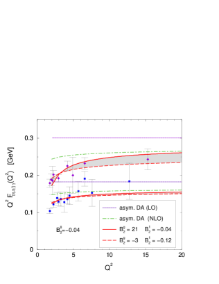
Figure 2: The scaled $P\gamma$ transition form factor vs. $Q^{2}$. Dotted (long-short dashed) lines represent the LO (NLO) predictions for the asymptotic distribution amplitudes. Solid (dashed) lines are results obtained with $B_{2}^{g}(\mu^{2}_{0})=21$ (-3), $B_{2}^{1}(\mu^{2}_{0})=-0.04$ (-0.12) and $B_{2}^{8}(\mu^{2}_{0})=-0.04$ ($\mu^{2}_{F}=Q^{2}$, $\mu^{2}_{R}=Q^{2}/2$, $\mu^{2}_{0}=1~{}{\rm GeV}^{2}$). The shaded areas indicate the range of the NLO predictions for $B_{2}^{1}$ and $B_{2}^{g}$ inside the allowed region (see text). Data taken from CLEO97 ; L398 (rhombs represent the $Q^{2}F_{\eta^{\prime}\gamma}$ data, squares the $Q^{2}F_{\eta\gamma}$ ones).

Next let us inspect the Gegenbauer expansion of the transition form factor. For $x$-independent factorization and renormalization scales the integrations involved in (LABEL:eq:Resetatff) and (LABEL:eq:tffeta8) can be performed analytically leading to the expansion

$$F^{1}_{P\gamma}(Q^{2}) = \frac{6\,f_{P}^{1}\,C_{1}}{Q^{2}}\;\bigg{\{}1+B_{2}^{1}(\mu^{2}_{F})+B_{4}^{1}(\mu^{2}_{F})$$

$$-\frac{5}{3}\frac{\alpha_{s}(\mu^{2}_{R})}{\pi}\,\left[1-B_{2}^{1}(\mu^{2}_{F})\,\left(\frac{59}{72}-\frac{5}{6}\ln{\frac{Q^{2}}{\mu^{2}_{F}}}\right)\right.$$

$$\left.\>\>-B_{4}^{1}(\mu^{2}_{F})\,\left(\frac{10487}{4500}-\frac{91}{75}\ln{\frac{Q^{2}}{\mu^{2}_{F}}}\right)\right.$$

$$\left.\>\>+B_{2}^{g}(\mu^{2}_{F})\left(\frac{55}{1296}-\frac{1}{108}\ln\frac{Q^{2}}{\mu^{2}_{F}}\right)\right.$$

$$\left.\>\>+B_{4}^{g}(\mu^{2}_{F})\left(\frac{581}{10125}-\frac{7}{675}\ln\frac{Q^{2}}{\mu^{2}_{F}}\right)\right]+\cdots\bigg{\}}\,.$$

Particle independence of the distribution amplitudes is used in this expansion. A similar expansion holds for the octet contribution with the obvious replacements $f_{P}^{1}\to f_{P}^{8}$, $B_{n}^{1}\to B_{n}^{8}$, and $B_{n}^{g}\to 0$. The expansion of the octet contribution is analogous to that one of the $\pi\gamma$ transition form factor MelicNP01 ; DiehlKV01 .

In the expansion (LABEL:eq:Tffactors) one notes a strong linear correlation between $B_{2}^{i}$ and $B_{4}^{i}$, only the mild logarithmic $Q^{2}$ dependence due to evolution and the running of $\alpha_{s}$ restricts their values to a finite region in parameter space. The gluon contributions to the form factors are strongly suppressed, they appear only to NLO and the numerical factors multiplying their Gegenbauer coefficients are small. The coefficients $B_{2}^{g}$ and $B_{4}^{g}$ are also correlated.

With regard to these correlations and in view of the errors of the experimental data CLEO97 ; L398 as well as the rather restricted range of momentum transfer in which they are available, we are forced to truncate the Gegenbauer series at $n=2$. Truncating at $n=4$ does not lead to reliable results in contrast to the simpler case of the pion where this is possible DiehlKV01 . A fit to the CLEO and L3 data for $Q^{2}$ larger then $2~{}{\rm GeV}^{2}$ provides

$$B_{2}^{8}(\mu^{2}_{0}) = -0.04\pm 0.04\,,$$

$$B_{2}^{1}(\mu^{2}_{0}) = -0.08\pm 0.04\,,$$

$$B_{2}^{g}(\mu^{2}_{0}) = \phantom{-}9\pm 12\,,$$ (62)

where the values of the Gegenbauer coefficients are obtained for the factorization scale $\mu^{2}_{F}=Q^{2}$. We repeat that $\mu^{2}_{0}=1~{}{\rm GeV}^{2}$ and the gluonic Gegenbauer coefficient is quoted for the normalization $\sigma=\sqrt{n_{f}/C_{F}}$. For comparison we also determine the Gegenbauer coefficients for $\mu^{2}_{F}=Q^{2}/2$; the values found agree with those quoted in (62) almost perfectly. The quality of the fit is shown in Fig. 2. The coefficients $B_{2}^{1}$ and $B_{2}^{g}$ are strongly correlated as can be seen from Fig. 3. The results (62) satisfy $\sqrt{2}|B_{2}^{8}(\mu^{2}_{F})-B_{2}^{1}(\mu^{2}_{F})|/3\ll 0.02$ for all $\mu^{2}_{F}>\mu^{2}_{0}$. This meets the requirement (60), and, therefore no substantial violations of the OZI rule follow from our distribution amplitudes. It moreover implies the approximative validity of the quark-flavor mixing scheme advocated for in Ref. FeldmannKS98 .

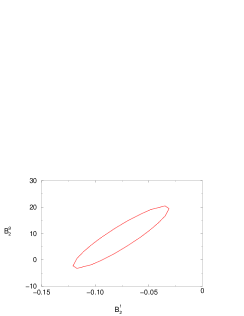
Figure 3: $1\sigma$ $\chi^{2}$-contour plot for the coefficients $B_{2}^{1}(\mu^{2}_{0})$ and $B_{2}^{g}(\mu^{2}_{0})$ obtained from a three-parameter fit to the CLEO and L3 data on the $\eta,\eta^{\prime}$–$\gamma$ transition form factors. Values of the Gegenbauer coefficients refer to $\mu^{2}_{0}=1~{}{\rm GeV}^{2}$; the factorization scale is $\mu^{2}_{F}=Q^{2}$.

In Fig. 4 we present the singlet and gluon distribution amplitudes at the scale $\mu^{2}_{0}$ obtained using the face values from (62). Both amplitudes are end-point suppressed as compared to the asymptotic one. This property holds for all values of $B_{2}^{1}$ and $B_{2}^{g}$ inside the allowed region (62).

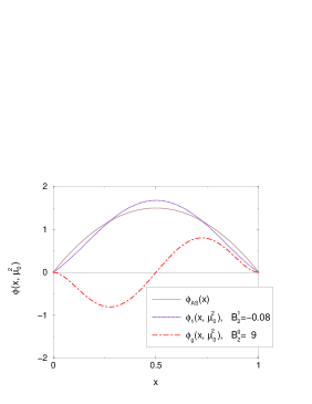
Figure 4: Flavour-singlet and gluon distribution amplitudes at the scale $\mu^{2}_{0}=1~{}{\rm GeV}^{2}$ obtained using the face values $B_{2}^{1}$ and $B_{2}^{g}$ from (62). The asymptotic distribution amplitude is included for comparison.

The values of $B_{2}^{1}$ and $B_{2}^{8}$ agree with each other within errors as well as with the Gegenbauer coefficient $B_{2}^{\pi}(\mu^{2}_{0})$ of the pion distribution amplitude for which a value of $-0.06\pm 0.03$ has been found in DiehlKV01 from an analysis along the same lines as our one. Thus, the three quark distribution amplitudes are very similar. This result explains the observation made in Feldmann99 and mentioned by us at the end of Sec. II D that the data on three transition form factors fall on top of each other within errors if the form factors are scaled by their respective asymptotic results (48). The $\eta_{c}\gamma$ transition form factor, on the other hand, behaves differently L399 . The $\eta_{c}$ mass provides a second large scale which cannot be ignored in the analysis FeldmannK97a .

We emphasize that our results on the $\eta$ and $\eta^{\prime}$ distribution amplitudes are to be considered as estimates performed with the purpose of getting an idea about the magnitude of the gluon distribution amplitude. As has been discussed in detail for the case of the $\pi\gamma$ transition form factor in DiehlKV01 , allowance of higher Gegenbauer coefficients in the analysis will change the result on $B_{2}^{\pi}$, essentially the sum of the $B_{n}^{\pi}$ is fixed by the data on the transition form factor. This ambiguity also holds for the case of the $\eta$ and $\eta^{\prime}$. Taking a lower renormalization scale than we do which may go along with a prescription for the saturation of $\alpha_{s}$ and thus including effects beyond a leading-twist analysis, will also change the results for the Gegenbauer coefficients. Another source of theoretical uncertainties in our analysis is the neglect of power and/or higher-twist corrections. Thus, for instance, in Refs. FeldmannK97 ; JKR the LO modified perturbative approach Sterman has been applied where quark transverse degrees of freedom and Sudakov suppressions are taken into account. In this case the asymptotic distribution amplitudes lead to good agreement with the data on the transition form factors.

V Comments on other hard reactions

In this section we make use of the results obtained in the preceding sections and calculate other hard processes involving $\eta$ and $\eta^{\prime}$ mesons in order to examine the role of the $gg$ Fock component further.

V.1 Electroproduction of $\eta,\eta^{\prime}$ mesons

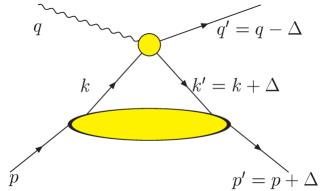
Figure 5: The handbag-type diagram for meson electroproduction off protons. The large blob represents a generalized parton distribution, the small one the subprocess $\gamma^{*}_{L}q\rightarrow P\,q$. The momentum transfer is $t=\Delta^{2}$.

As a first application of the gluon distribution amplitude extracted from the $\eta\gamma$ and $\eta^{\prime}\gamma$ transition form factors we calculate deeply virtual electroproduction of $\eta$ and $\eta^{\prime}$ mesons off protons. It has been shown Radyushkin96 ; CollinsFS96 that for large virtualities of the exchanged photon, $Q^{2}$, and small momentum transfer from the initial to the final proton, $t$, electroproduction of pseudoscalar mesons is dominated by longitudinally polarized virtual photons and the process amplitude factorizes into a parton-level subprocess $\gamma^{*}_{L}\,q\to Pq$ and soft proton matrix elements which represent generalized parton distributions MullerRGDH94 , see Fig. 5. The meson is generated by a leading-twist mechanism, i.e., by the transition $q\overline{q}\to P$ mediated through the exchange of a hard gluon. For the production of $\eta$ and $\eta^{\prime}$ mesons, however, one has to consider the gluon Fock component as well which, in contrast to the case of the transition form factors, contributes to the same order of $\alpha_{s}$ as the $q\overline{q}_{i}$ components. The gluonic contribution has not been considered in previous calculations of the electroproduction cross sections MankiewiczPW97 ; HuangK00 .

The helicity amplitude for the process $\gamma^{*}_{L}\,p\to Pp$ is again decomposed into flavor octet and singlet components, $q\overline{q}_{i}\to P$

$${\cal M}^{Pi}_{0\pm,0\pm} = \sum_{a}ee_{a}C_{a}^{\,i}\sqrt{1-\xi^{2}}\int_{-1}^{1}\,\frac{d\bar{x}}{\sqrt{\bar{x}^{2}-\xi^{2}}}\,{\cal H}^{Pi}_{0\pm,0\pm}$$ (63)

$$\times\left[\widetilde{H}^{a}(\bar{x},\xi,t)-\frac{\xi^{2}}{1-\xi^{2}}\widetilde{E}^{a}(\bar{x},\xi,t)\right]\,,$$

where $\widetilde{H}^{a}$ and $\widetilde{E}^{a}$ are the axial vector and pseudoscalar generalized parton distributions for the emission and reabsorption of quarks of flavor $a$. The $C_{a}^{i}$ are flavor factors for the $q\overline{q}_{i}$ components of the meson $P$; they can be read off from (81). The quark subprocess amplitudes $\gamma_{L}^{*}q\to q\overline{q}_{i}\,q$ are calculated from the LO Feynman diagrams for which examples are shown in Fig. 6 HuangK00

$${\cal H}^{Pi}_{0\pm,0\pm}(\hat{s},{t},Q^{2}) = \pm\,4\pi\alpha_{s}(\mu^{2}_{R})\frac{C_{F}}{N_{c}}\,f_{P}^{i}\,\frac{Q\sqrt{-\hat{u}\hat{s}}}{Q^{2}+\hat{s}}$$ (64)

$$\times\int_{0}^{1}\,d\tau\,\frac{\phi_{i}(\tau,\mu^{2}_{F})}{(1-\tau)Q^{2}-\tau t}\,$$

$$\times\left[1-\frac{\hat{u}}{\hat{s}}+\frac{1}{1-\tau}\frac{t}{\hat{u}}\right]\,.$$

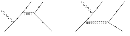
Figure 6: Sample leading order Feynman diagrams that contribute to the subprocess amplitude $\gamma^{*}_{L}q\rightarrow q\overline{q}_{i}\,q$.

They are expressed in terms of the subprocess Mandelstam variables $\hat{s},\hat{u},\hat{t}=t$ where $\hat{s}+t+\hat{u}=-Q^{2}$, and hold for any value of $Q^{2}$ and $t$. For the deeply virtual kinematical region of large $Q^{2}$ and $-t\ll Q^{2}$, it is more appropriate to use the scaling variables $\xi$ and $\bar{x}$. The skewness is defined by the ratio of light-cone plus components of the incoming ($p$) and outgoing ($p^{\prime}$) proton momenta

$$\xi=\frac{(p-p^{\,\prime})^{+}}{(p+p^{\,\prime})^{+}}\,.$$ (65)

For large $Q^{2}$ the skewness is related to $x$-Bjorken by $\xi\simeq x_{Bj}/2$. The average momentum fraction the emitted and reabsorbed partons carry, is defined as

$$\bar{x}=\frac{(k+k^{\prime})^{\,+}}{(p+p^{\prime})^{\,+}}\,.$$ (66)

Here, $k$ and $k^{\prime}$ are the momenta of the emitted and reabsorbed partons, respectively. For $-t\ll Q^{2}$ the Mandelstam variables are related to the skewness and the average momentum fraction

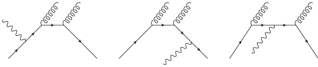
Figure 7: Representative LO Feynman diagrams that contribute to the subprocess amplitude $\gamma^{*}_{L}q\rightarrow gg\,q$.

$$\hat{s}=\frac{Q^{2}}{2\xi}(\bar{x}-\xi)\,,\qquad\hat{u}=-\frac{Q^{2}}{2\xi}(\bar{x}+\xi)\ \,.$$ (67)

Rewriting the subprocess amplitude in terms of $\xi$ and $\bar{x}$ and inserting the result into the factorization formula (63), one arrives at the well-known result for the leading-twist contribution to deeply virtual electroproduction of pseudoscalar mesons MankiewiczPW97

$${\cal M}^{Pi}_{0\pm,0\pm}(Q^{2},\xi,t\simeq 0)$$ (68)

$$= \pm\frac{4\pi\alpha_{s}(\mu^{2}_{R})}{Q}\,\frac{C_{F}}{N_{c}}\,f_{P}^{i}\sqrt{1-\xi^{2}}\int_{0}^{1}d\tau\frac{\phi_{i}(\tau,\mu^{2}_{F})}{\tau}\,$$

$$\times\sum_{a}ee_{a}C_{a}^{i}\>\int_{-1}^{1}\,{d\bar{x}}\left[\frac{1}{\bar{x}+\xi-i\varepsilon}+\frac{1}{\bar{x}-\xi+i\varepsilon}\right]$$

$$\times\left[\widetilde{H}^{a}(\bar{x},\xi,t)-\frac{\xi^{2}}{1-\xi^{2}}\widetilde{E}^{a}(\bar{x},\xi,t)\right]\,.$$

Next we calculate the subprocess amplitude for the gluonic component of the meson, $\gamma^{*}_{L}\,q\to gg\,q$. There are six graphs that contribute to the subprocess. Three representative ones are depicted in Fig. 7, the other three ones are obtained from these by interchanging the gluons. We find for that subprocess amplitude the result

$${\cal H}^{Pg}_{0\pm,0\pm}(\hat{s},t,Q^{2}) = \mp 4\pi\alpha_{s}(\mu^{2}_{R})\,\frac{f_{P}^{1}}{\sqrt{n_{f}}}\,\frac{C_{F}}{N_{c}}\,\frac{Q}{Q^{2}+\hat{s}}\,\frac{-t}{\sqrt{-\hat{u}\hat{s}}}$$ (69)

$$\times\,\int_{0}^{1}d\tau\,\frac{\phi_{g}(\tau,\mu^{2}_{F})}{\tau^{2}(1-\tau)}\,.$$

In deriving this expression we made use of the antisymmetry of the gluon distribution amplitude (88). The gluonic contribution to the $\gamma^{*}_{L}\,p\to Pp$ helicity amplitudes reads

$${\cal M}^{Pg}_{0\pm,0\pm} = \sum_{a}ee_{a}\sqrt{1-\xi^{2}}\,\int_{-1}^{1}\,\frac{d\bar{x}}{\sqrt{\bar{x}^{2}-\xi^{2}}}\,\,{\cal H}^{Pg}_{0\pm,0\pm}$$ (70)

$$\times \left[\widetilde{H}^{a}(\bar{x},\xi,t)-\frac{\xi^{2}}{1-\xi^{2}}\,\widetilde{E}^{a}(\bar{x},\xi,t)\right]\,.$$

The full $\gamma^{*}_{L}\,p\to Pp$ amplitudes are the sum of the flavor octet and singlet contributions (68) and the gluonic one (70). In the deeply virtual region, however, the gluon contribution is suppressed by $t/Q^{2}$ as one readily observes from (69). It is, therefore, to be considered as a power correction to the leading quark contribution (68) and is to be neglected in a leading-twist analysis of deeply virtual electroproduction of $\eta$ and $\eta^{\prime}$ mesons.

One may also consider wide-angle photo- and electroproduction of $\eta$ and $\eta^{\prime}$ mesons. Using the methods proposed in DiehlFJK98 for wide-angle Compton scattering, one can show that for wide-angle photo- and electroproduction of pseudoscalar mesons the factorization formulas (63) and (70) hold as well provided $-t$ and $-u$ are large as compared to the square of the proton mass and $Q^{2}\ll-t$ HuangK00 . To show that one has to work in a symmetric frame in which the skewness is zero. One can also show that, in this situation, $\hat{s}$ and $\hat{u}$ are approximate equal to the Mandelstam variables for the full process, $s$ and $u$, respectively. Thus, in the wide-angle region and for $Q^{2}\ll-t,s$ but non-zero, (63) and (70) simplify to

$${\cal M}^{Pi}_{0\pm,0\pm}(s,t,Q^{2}\ll-t) = e\,{\cal H}^{Pi}_{0\pm,0\pm}\sum_{a}e_{a}C_{a}^{i}R_{A}^{a}(t)\,,$$

$${\cal M}^{Pg}_{0\pm,0\pm}(s,t,Q^{2}\ll-t) = e\,{\cal H}^{Pg}_{0\pm,0\pm}\sum_{a}e_{a}R_{A}^{a}(t)\,,$$

where the form factors $R_{A}^{a}$ represent $1/\bar{x}$ moments of the generalized parton distributions $\widetilde{H}^{a}$ at zero skewness. These form factors also contribute to wide-angle Compton scattering DiehlFJK98 . The amplitudes for transversally polarized photons can be obtained analogously. In contrast to the case of deeply virtual electroproduction MankiewiczP99 , factorization for these amplitudes holds in the wide-angle region, too.

In order to estimate the size of the gluon contribution to wide-angle electroproduction of $\eta,\eta^{\prime}$ mesons, we plot in Fig. 8 the ratio

$$\frac{{\cal M}^{Pg}_{0\pm,0\pm}}{{\cal M}^{P1}_{0\pm,0\pm}} = \frac{-t^{2}}{2s^{2}+t^{2}+ts}$$

$$\times\int_{0}^{1}d\tau\frac{\phi_{g}(\tau,\mu^{2}_{F})}{\tau^{2}(1-\tau)}\left[\int_{0}^{1}d\tau\frac{\phi_{1}(\tau,\mu^{2}_{F})}{\tau}\right]^{-1}\,,$$

evaluated from the distribution amplitudes (62) for which the ratio of the integrals is $\simeq-5\,B_{2}^{g}(\mu^{2}_{F})/18$. The ratio may be large in particular in the backward hemisphere. Thus, at least for electroproduction of $\eta^{\prime}$ mesons the $gg$ Fock component should be taken into account for sufficiently large momentum transfer. For the production of the $\eta$ meson it plays a minor role since $\eta$ production is dominated by the flavor-octet contribution ($f_{\eta}^{1}/f_{\eta}^{8}=0.16$). Note, however, that the normalization of the meson electroproduction in both the regions, the deeply virtual and the wide-angle one, is not well understood in the kinematical region accessible to present day experiments.

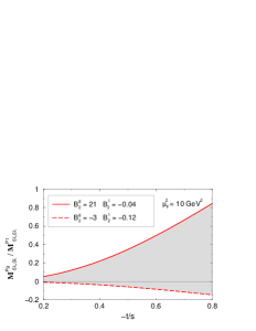
Figure 8: Ratio of gluon and flavor-singlet quark amplitudes for wide-angle electroproduction of $\eta$ or $\eta^{\prime}$ mesons ($\mu^{2}_{F}=10~{}{\rm GeV}^{2}$). The shaded area indicates the range of predictions evaluated from $B_{2}^{1}(\mu^{2}_{0})$ and $B_{2}^{g}(\mu^{2}_{0})$ inside the allowed region according to Fig. 3.

V.2 The $g^{*}g^{*}P$ vertex

A reliable determination of the $g^{*}g^{*}\eta^{\prime}$ vertex is of importance for the calculation of a number of decay processes such as $B\to\eta^{\prime}K$, $B\to\eta^{\prime}X_{s}$, or of the hadronic production process $pp\to\eta^{\prime}X$. The $g^{*}g^{*}\eta^{\prime}$ vertex has been calculated by two groups recently MutaY99 ; AliP00 . We reanalyze this vertex to leading-twist order using our set of conventions. This will allow us to examine the previous calculations, and provide predictions for $Pg^{*}$ transition form factor using the Gegenbauer coefficients (62) in the distribution amplitudes.

We define the gluonic vertex in analogy to the electromagnetic one , see (5), as

$$\Gamma^{\mu\nu}_{ab}=i\;F_{Pg^{*}}(\overline{Q}^{\,2},\omega)\;\delta_{ab}\;\epsilon^{\mu\nu\alpha\beta}\;q_{1\alpha}q_{2\beta}$$ (73)

where $q_{1}$ and $q_{2}$ denote the momenta of the gluons now and $a$ and $b$ label the color of the gluon. It is evident that the transition to a colorless meson requires the same color of both the gluons. We consider space-like gluon virtualities for simplicity; the generalization to the case of time-like gluons is straightforward. We introduce an average virtuality and an asymmetry parameter by

$$\overline{Q}^{\,2}=-\frac{1}{2}(q_{1}^{2}+q_{2}^{2})\,,\qquad\omega=\frac{q_{1}^{2}-q_{2}^{2}}{q_{1}^{2}+q_{2}^{2}}\,.$$ (74)

The values of $\omega$ range from $-1$ to $1$, but due to Bose symmetry the transition form factor is symmetric in this variable: $F_{Pg^{*}}(\overline{Q}^{\,2},\omega)=F_{Pg^{*}}(\overline{Q}^{\,2},-\omega)$.

The calculation of the transition form factor to leading twist accuracy and lowest order in $\alpha_{s}$ parallels that of the meson-photon transition form factor which we presented in some detail in Sec. II. In contrast to the electromagnetic case, however, already to the lowest order in $\alpha_{s}$ the two partonic subprocesses $g^{*}g^{*}\to q\bar{q}$ and $g^{*}g^{*}\to gg$ contribute. The relevant Feynman diagrams are shown in Fig. 9. There are a few more diagrams which involve the triple and quadruple gluon vertices. The contributions from these diagrams are separately zero when contracted with either the $q\overline{q}$ or the $gg$ projectors (91), (41).

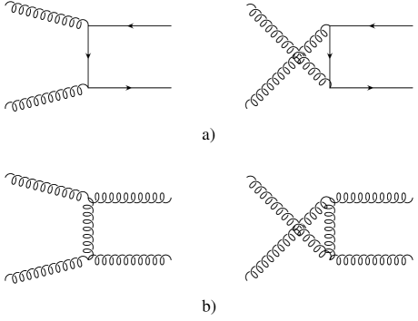
Figure 9: Relevant lowest order Feynman diagrams for the $g^{*}g^{*}\to q\overline{q}$ (a) and $g^{*}g^{*}\to gg$ subprocess (b).

The following result for the $Pg^{*}$ transition form factor can readily be obtained

$$F_{Pg^{*}}(\overline{Q}^{\,2},\omega) = 4\pi\alpha_{s}(\mu^{2}_{R})\;\frac{f_{P}^{1}}{\overline{Q}^{\,2}}\;\>\frac{\sqrt{n_{f}}}{N_{c}}\;$$

$$\times\left[A_{q\overline{q}}(\omega)+\frac{N_{c}}{2n_{f}}\,A_{gg}(\omega)\right]+{\cal O}(\alpha_{s}^{2})\,,$$

where

$$A_{q\overline{q}}(\omega) = \int_{0}^{1}dx\,\phi_{1}(x,\mu_{F}^{2})\;\frac{1}{1-\omega^{2}(1-2x)^{2}}\,,$$

$$A_{gg}(\omega) = \int_{0}^{1}dx\,\frac{\phi_{g}(x,\mu_{F}^{2})}{x\overline{x}}\;\frac{1-2x}{1-\omega^{2}(1-2x)^{2}}\,.$$

There is no contribution from the $q\overline{q}_{8}$ component to this vertex.

Inserting the Gegenbauer expansions (LABEL:eq:solphi) into (LABEL:eq:ourAqqgg) the integrals can be performed analytically term by term analogously to (LABEL:eq:Tffactors) resulting in the expansions

$$A_{q\overline{q}}(\omega) = c_{0}(\omega)+c_{2}(\omega)\;B^{1}_{2}(\mu^{2}_{F})+\cdots\,,$$

$$A_{gg}(\omega) = g_{2}(\omega)\;B_{2}^{g}(\mu^{2}_{F})+\cdots\,,$$ (77)

where

$$c_{0}(\omega) = \frac{3}{2\omega^{2}}\left[1-\frac{1}{2\omega}\left(1-\omega^{2}\right)\ln\frac{1+\omega}{1-\omega}\right]\,,$$

$$c_{2}(\omega) = \frac{3}{4\omega^{4}}\left[15-13\omega^{2}-\frac{3}{2\omega}\left(5-6\omega^{2}+\omega^{4}\right)\ln\frac{1+\omega}{1-\omega}\right]\,,$$

$$g_{2}(\omega) = \frac{-5}{12\omega^{4}}\left[3-2\omega^{2}-\frac{3}{2\omega}\left(1-\omega^{2}\right)\ln\frac{1+\omega}{1-\omega}\right]\,.$$

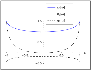
Figure 10: Functions $c_{0}$, $c_{2}$, and $g_{2}$, defined in Eq. (LABEL:eq:c0c2g2), vs. $\omega$.

The behaviour of functions $c_{0}(\omega)$, $c_{2}(\omega)$, and $g_{2}(\omega)$ is illustrated in Fig. 10. Examining the function $c_{2}(\omega)$ and Eq. (77), one notice that the form factors become increasingly less sensitive to the coefficients $B_{2}^{1}(\mu^{2}_{F})$ with decreasing $|\omega|$. This behaviour is characteristic of all functions $c_{n}(\omega)$ ($n>0$) DiehlKV01 . On the other hand, the functions $c_{0}(\omega)$ and $g_{2}(\omega)$ do not depend so drastically on $\omega$ and they are non-zero at $\omega=0$. One can easily show that all $g_{n}(\omega)$, for $n>0$ and even, possess this property.

Let us discuss two interesting limiting cases. For $\omega\ll 1$, i.e., for $q_{1}^{2}\approx q_{2}^{2}$, the form factors behave as

$$F_{Pg^{*}}(\overline{Q}^{\,2},\omega) = \frac{4\pi\alpha_{s}(\mu^{2}_{R})}{\sqrt{3}\;\overline{Q}^{\,2}}\;f_{P}^{1}\;\left[1-\frac{1}{12}B_{2}^{g}(\mu^{2}_{F})\right.$$ (79)

$$\left.+\frac{1}{5}\omega^{2}\left(1+\frac{12}{7}B_{2}^{1}(\mu^{2}_{F})-\frac{5}{28}B_{2}^{g}(\mu^{2}_{F})\right)\right]$$

$$+\,{\cal O}(\omega^{4},\alpha_{s}^{2})\,.$$

Thus, the limiting value for $\omega\to 0$ is sensitive to the form of the gluon distribution amplitude while it does not depend on the Gegenbauer coefficients of the quark one. This is to be contrasted with the $P\gamma^{*}$ transition form factor which, according to DiehlKV01 , is independent of both the quark and the gluonic Gegenbauer coefficients in the limit $\omega\to 0$.

For $\omega\to\pm 1$, i.e., in the limit where one of the gluons goes on-shell, the $Pg$ transition form factor becomes

$$F_{Pg}(Q^{2},\omega=\pm 1) = \frac{4\sqrt{3}\pi\alpha_{s}(\mu^{2}_{R}))}{Q^{2}}\;f_{P}^{1}\;$$ (80)

$$\times\left[1+B_{2}^{1}(\mu^{2}_{F})-\frac{5}{36}B_{2}^{g}(\mu^{2}_{F})\right]$$

$$+\,{\cal O}(\alpha_{s}^{2})\,,$$

where $Q^{2}=-q_{1}^{2}\,(-q_{2}^{2})$ as in the electromagnetic case. In Fig. 11 we display our predictions for the scaled $\eta^{\prime}g^{*}$ transition form factor evaluated from the distribution amplitudes determined in Sec. IV, choosing $\mu^{2}_{F}=\mu^{2}_{R}=\overline{Q}^{2}$. Given the large difference in the magnitude of $B_{2}^{1}(\mu^{2}_{0})$ and $B_{2}^{g}(\mu^{2}_{0})$, see (62), we observe a strong sensitivity of the $Pg$ transition form factors on the gluon distribution amplitude in contrast to the electromagnetic case. Due to the badly determined coefficient $B_{2}^{g}$ the uncertainties in the predictions for $F_{\eta^{\prime}g^{*}}$ are large. Because of the smallness of the mixing angle $\theta_{1}$, see (52) and (53), the $\eta g^{*}$ transition form factor is much smaller then the $\eta^{\prime}g^{*}$ one. The ratio of the two form factors, $F_{\eta g^{*}}(\overline{Q}^{2},\omega)/F_{\eta^{\prime}g^{*}}(\overline{Q}^{2},\omega)$ is given by $-\tan\theta_{1}$. This result offers a way to measure the angle $\theta_{1}$ as has been pointed out in FeldmannKS98 .

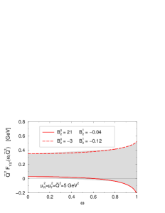
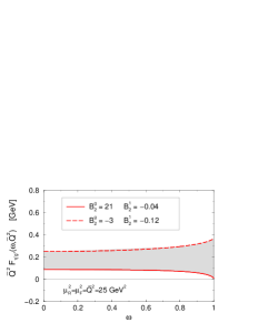
Figure 11: Predictions for the $\eta^{\prime}g^{*}$ transition form factor as a function of $\omega$ for two values of $\overline{Q}^{2}$. The shaded areas indicate the range of predictions evaluated from $B_{2}^{1}(\mu^{2}_{0})$ and $B_{2}^{g}(\mu^{2}_{0})$ inside the allowed region according to Fig. 3.

Let us compare our results for the $\eta^{\prime}g^{*}$ transition form factors with those presented in Refs. MutaY99 ; AliP00 . First we remark that there is perfect agreement for the contribution from the meson’s $q\overline{q}_{1}$ component. As for the contribution from the gluonic component we differ by a factor $1/(2n_{f})$ from Refs. MutaY99 ; AliP00 . Furthermore, in AliP00 , there is an additional factor of $\omega$ multiplying the gluonic term rendering it antisymmetric in $\omega$ in conflict with Bose symmetry. We suspect that a gluonic projector $\sim\varepsilon^{\mu\nu\alpha\beta}q_{1\alpha}q_{2\beta}/\overline{Q}^{2}$ is used in AliP00 which turns into $\sim\omega\varepsilon^{\mu\nu}_{\perp}$ in a frame where the meson moves along the 3-direction. This is in conflict with (92), (93) except at $\omega=1$.

The origin of the missing factor $1/(2n_{f})$ is not easy to discover since in Refs. MutaY99 ; AliP00 the form of the gluonic projector is not specified. Given the anomalous dimensions quoted in MutaY99 ; AliP00 , which are the same as in (40), this incriminated factor cannot be assigned to a particular normalization of the gluonic projector, (41) must be applied. On the other hand, using $\sigma=1/(2\sqrt{n_{f}\,C_{F}})$ as the normalization of the gluonic projector, the results for the transition form factors given in MutaY99 ; AliP00 would be correct (ignoring the problem with the factor $\omega$ in AliP00 ), provided the corresponding anomalous dimensions are applied, see (36), and they differ from the ones quoted in these papers. Hence, the quoted anomalous dimensions and the result for the gluon part of the hard-scattering amplitude seem not to be in agreement.

In Ref. DiehlKV01 the leading term of the expansion (79) has been derived from the results presented in AliP00 and it therefore disagrees with our result.

VI Summary

In this work we have investigated the two-gluon Fock components of the $\eta$ and $\eta^{\prime}$ mesons to leading-twist accuracy. Since the integral over the gluon distribution amplitude is zero, see (4), there is no natural normalization of it in contrast to the case of the $q\overline{q}$ distribution amplitudes. Any choice of this normalization goes along with corresponding normalizations of the anomalous dimensions and the projector of a two-gluon state onto a pseudoscalar meson. We have set up a consistent set of conventions for the three quantities which is imperative for leading-twist calculations of hard exclusive reactions involving $\eta$ and/or $\eta^{\prime}$ mesons. We have also compared this set with other conventions to be found in the literature.

As an application of the two-gluon components we have calculated the flavor-singlet part of the $\eta\gamma$ and $\eta^{\prime}\gamma$ transition form factors to NLO in $\alpha_{s}$ and explicitly shown the cancellation of the collinear singularities present in the hard scattering amplitude with the UV one occurring in the unrenormalized distribution amplitudes. Assuming particle independence of the distribution amplitudes, we have employed the results for the transition form factors in an analysis of the available data CLEO97 ; L398 and determined the Gegenbauer coefficients to order $n=2$ for the three remaining distribution amplitudes, the flavor octet, singlet and gluon one. The numerical results for the distribution amplitudes quoted for $\sigma=\sqrt{n_{f}/C_{F}}$ are in agreement with the quark flavor mixing scheme proposed in FeldmannKS98 .

The value for the lowest order gluonic Gegenbauer coefficient is subject to a rather large error since the contributions from the two-gluon Fock components to the transition form factors are suppressed by $\alpha_{s}$ as compared to the $q\overline{q}$ contributions. This suppression does not necessarily occur in other hard exclusive reactions; examples of such reactions, discussed by us briefly, are deeply virtual and wide-angle electroproduction of $\eta$ or $\eta^{\prime}$ mesons as well as the $g^{*}g^{*}\eta(\eta^{\prime})$ vertex. The latter two reactions, as it has turned out, are actually quite sensitive to the two-gluon components and future data for them should allow to pin down the gluon distribution amplitude more precisely than it is possible from the transition form factor data. Other hard exclusive reactions which may be of relevance to our considerations are, for instance, the decays $\chi_{cJ}\to\eta\eta,\eta^{\prime}\eta^{\prime}$ BolzKS96 ; BaierG85a or $B\to\eta^{(}{}^{\prime}{}^{)}K^{(*)}$ beneke . Last not least we would like to mention that the two-gluon components of other flavor-neutral mesons or even those of glueballs carlson can be studied in full analogy to the $\eta$-$\eta^{\prime}$ case.

Appendix A Definitions of meson states and distribution amplitudes

The flavor content of the neutral pseudoscalar meson states we are interested in, is taken into account by

$$\begin{array}[]{llcl}\pi^{0}:&\displaystyle\frac{1}{\sqrt{2}}(u\bar{u}-d\bar{d})&\rightarrow&\;\displaystyle{\cal C}_{3}=\frac{1}{\sqrt{2}}\,\lambda_{3}\,,\\[11.38092pt] q\overline{q}_{8}:&\displaystyle\frac{1}{\sqrt{6}}(u\bar{u}+d\bar{d}-2s\bar{s})&\rightarrow&\;\displaystyle{\cal C}_{8}=\frac{1}{\sqrt{2}}\,\lambda_{8}\,,\\[11.38092pt] q\overline{q}_{1}:&\displaystyle\frac{1}{\sqrt{3}}(u\bar{u}+d\bar{d}+s\bar{s})&\rightarrow&\;\displaystyle{\cal C}_{1}=\frac{1}{\sqrt{n_{f}}}\,\mathbf{1}_{f}\,,\end{array}$$ (81)

where $\lambda_{i}$ are the usual $SU(3)$ Gell-Mann matrices and $\mathbf{1}$ is the $3\times 3$ unit matrix. For the flavor-singlet state, we use the general notation Terentev81 in which the flavor content is expressed in terms of $n_{f}$ which denotes the number of flavors contained in $q\overline{q}_{1}$ ($n_{f}=3$ in our case). This simplifies the comparison with the results for kernels to be found in the literature.

As usual LepageB80 ; BrodskyDFL86 ; ChernyakZ84 we define the distribution amplitudes in a frame where the meson moves along the 3-direction. Neglecting the meson’s mass its momentum reads

$$p=[p^{+},0,\mathbf{0}_{\perp}]\,,$$ (82)

where we use light-cone coordinates $v=[v^{+},v^{-},\mathbf{v}_{\perp}]$ with $v^{\pm}=(v^{0}\pm v^{3})/\sqrt{2}$ for any four-vector $v$ . We also introduce a light-like vector

$$n=[0,1,\mathbf{0}_{\perp}]\,.$$ (83)

which defines the plus component of a vector, $v^{+}=n\cdot v$. The constituents of the meson, quarks or gluons, carry the fractions $u$ and $1-u$ of the light-cone plus components of the meson’s momentum. The distribution amplitudes are defined by Fourier transforms of hadronic matrix elements

$$\Phi_{Pi}(u) = \frac{f_{P}^{i}}{2\sqrt{2N_{c}}}\,\phi_{Pi}(u)$$ (84)

$$= -i\int\frac{dz^{-}}{2\pi}e^{i(u-(1-u))p\cdot z}\;\left<0\left|\overline{\Psi}(-z)\;{\cal C}_{i}\;\frac{n/\gamma_{5}}{\sqrt{2N_{c}}}\;\Omega\,\Psi(z)\right|P\,(p)\right>\,,$$

and

$$\Phi_{Pg}(u) = \frac{f_{P}^{1}}{2\sqrt{2N_{c}}}\,\phi_{Pg}(u)$$ (85)

$$= \frac{2}{(n\cdot p)}\int\frac{dz^{-}}{2\pi}e^{i(u-(1-u))p\cdot z}\;\frac{n_{\mu}n_{\nu}}{\sqrt{N_{c}^{2}-1}}\;\left<0\left|G^{\mu\alpha}(-z)\,\Omega\,\widetilde{G}_{\alpha}^{\>\>\>\nu}(z)\right|P\,(p)\right>\,,$$

where $z=[0,z^{-},\mathbf{0}_{\perp}]$. Here, $\Psi$ denotes a quark field operator, $G^{\mu\nu}$ the gluon field strength tensor, and $\widetilde{G}^{\mu\nu}$ its dual

$$\widetilde{G}^{\mu\nu}=\frac{1}{2}\;\epsilon^{\mu\nu\alpha\beta}\;G_{\alpha\beta}\,.$$ (86)

The quark and gluon operators in Eqs. (84), (85) are understood as color summed. The path-ordered factor

$$\Omega=\mbox{exp}\left\{ig\int_{-1}^{1}dsA(zs)\cdot z\right\}\,,$$ (87)

where $A$ is the gluon field, renders $\phi_{Pi}$ and $\phi_{Pg}$ gauge invariant. The distribution amplitudes in (84, 85) represent either the unrenormalized ones ($\phi^{ur}_{Pi,g}(u)$) if defined in terms of unrenormalized quark or gluonic composite operators or the renormalized one. In the latter case the distribution amplitudes are scale dependent ($\phi_{Pi,g}(u,\mu^{2})$). The distribution amplitudes defined above satisfy the symmetry relations

$$\phi_{P1,8}(u,\mu^{2}) = \phi_{P1,8}(1-u,\mu^{2})\,,$$

$$\phi_{Pg}(u,\mu^{2}) = -\phi_{Pg}(1-u,\mu^{2})\,.$$ (88)

The definitions of the distribution amplitudes (84) and (85) can be inverted to

$$\left<0\left|\overline{\Psi}(-z)\;{\cal C}_{i}\;n/\gamma_{5}\;\Omega\,\Psi(z)\right|P\right>$$ (89)

$$\qquad= i\,n\cdot p\,f_{P}^{i}\int_{0}^{1}du\;e^{-i(2u-1)\,p\cdot z}\>\phi_{Pi}(u)\>\,,\qquad$$

and

$$\;n_{\mu}n_{\nu}\;\left<0\left|G^{\mu\alpha}(-z)\,\Omega\,\widetilde{G}_{\alpha}^{\>\>\>\nu}(z)\right|P\right>$$

$$= \frac{1}{2}(n\cdot p)^{2}\,\sqrt{C_{F}}\,f_{P}^{1}\,\int_{0}^{1}du\;e^{-i(2u-1)\,p\cdot z}\>\phi_{Pg}(u)\>\,.$$

The projection of a collinear $q\bar{q}$ state onto a pseudoscalar meson state is achieved by replacing the quark and antiquark spinors (normalized as $u^{\dagger}(p,\lambda)u(p,\lambda^{\prime})=\sqrt{2}n\cdot p\,\delta_{\lambda\lambda^{\prime}}$) by LepageB80

$${\cal P}^{i,q}_{\alpha\beta,rs,kl}={\cal C}_{i,rs}\frac{\delta_{kl}}{\sqrt{N_{c}}}\left(\frac{\gamma_{5}\not\!p}{\sqrt{2}}\right)_{\alpha\beta}\,,$$ (91)

where $\alpha$ ($r$, $k$) and $\beta$ ($s$, $l$) represent Dirac (flavor, color) labels of the quark and antiquark, respectively. When calculating amplitudes, the projector (91) leads to traces. The projector holds for both incoming and outgoing states and corresponds to the definition of the the quark distribution amplitudes (84). It is to be used in calculations of hard-scattering amplitudes which are to be convoluted with $f_{P}^{i}/(2\sqrt{2N_{c}})\phi_{Pi}$ subsequently.

The form of the projection of a $gg$ state on a pseudoscalar state with momentum $p$ can be deduced by noting that the helicity zero combination of transversal gluon polarization vectors $\epsilon^{\mu}$ can be written as DiehlFJK00

$$\begin{array}[]{l}\epsilon^{\mu}(up,\lambda)\epsilon^{\nu}((1-u)p,-\lambda)-\epsilon^{\mu}(up,-\lambda)\epsilon^{\nu}((1-u)p,\lambda)\\[4.26773pt] \qquad=i\,\mbox{sign}(\lambda)\,\varepsilon_{\perp}^{\mu\nu}\,,\end{array}$$ (92)

where $\varepsilon^{12}_{\perp}=-\varepsilon^{21}_{\perp}=1$ while all other components of the transverse polarization tensor are zero. It can be expressed by

$$\varepsilon_{\perp}^{\mu\nu}=\varepsilon^{\mu\nu\alpha\beta}\;\frac{n_{\alpha}p_{\beta}}{n\cdot p}\,.$$ (93)

Instead of $n$ any other four vector can be used in (93) that has a non-zero minus and a vanishing transverse component. The projector of an state of two incoming collinear gluons of color $a$ and $b$ and Lorentz indices $\mu$ and $\nu$, associated with the momentum fractions $u$ and $(1-u)$, respectively, onto a pseudoscalar meson state reads

$${\cal P}^{g}_{\mu\nu,ab}=\frac{i}{2}\;\frac{\delta_{ab}}{\sqrt{N_{c}^{2}-1}}\;\frac{\varepsilon_{\perp\mu\nu}}{u(1-u)}\,.$$ (94)

The complex conjugated expression is to be taken for an outcoming $gg$ state. The projector is to be used along with the distribution amplitude $f_{P}^{i}/(2\sqrt{2N_{c}})\phi_{Pg}$. The additional factor $[u(1-u)]^{-1}$ appearing as part of the projector, is a consequence of the fact that in perturbative calculations of reactions involving two-gluon Fock components, the potential $A$ of the gluon field occurs, while the gluon distribution amplitude is defined in terms of the gluon field strength operator, see (85). The conversion from a matrix element of field strength tensors (LABEL:eq:melemg1u) to one of potentials is given by Radyushkin96 ; Kogut

$$\left<0\left|A^{\alpha}(-z)\,A^{\beta}(z)\right|P\right>$$ (95)

$$\>= \frac{1}{4}\varepsilon^{\alpha\beta}_{\perp}\,\sqrt{C_{F}}\,f_{P}^{1}\,\int_{0}^{1}du\;e^{-i(2u-1)\,p\cdot z}\frac{\phi_{Pg}(u)}{u(1-u)}\,.\qquad\quad$$

The gluonic projector (94) is obtained (up to the factor $[u(1-u)]^{-1}$ explained above) by the coupling of two collinear gluons into a colorless pseudoscalar state. In the context of mixing under evolution another normalization of it appears to be more appropriate, see (41). This normalization is accompanied by corresponding changes in the gluon distribution amplitude $\phi_{Pg}$ and the anomalous dimensions, as is discussed in detail in Sec. II.

For Levi-Civita tensor we use the convention

$$\varepsilon^{0123}=-1\,,$$ (96)

which leads to

$$\textnormal{Tr}\left[\gamma_{5}\gamma^{\mu}\gamma^{\nu}\gamma^{\alpha}\gamma^{\beta}\right]=4i\varepsilon^{\mu\nu\alpha\beta}\,$$ (97)

(with $\gamma_{5}=i\gamma^{0}\gamma^{1}\gamma^{2}\gamma^{3}$).

Appendix B The $P\gamma$ transition form factor -
details of the calculation

In this appendix, we provide some details of the calculation of the evolution kernels and the hard scattering amplitude for the flavor-singlet contribution to the $P\gamma$ transition form factor. These quantities can, in principle, be taken from the literature (see, e.g. Terentev81 ; BaierG81 and DVCS ) but the conventions and notations differ. However, since it is imperative to use a consistent set of conventions for the hard scattering amplitude and the distribution amplitudes, we recalculate them. In doing so we follow closely Ref. MelicNP01 . Dimensional regularization in $D=4-2\epsilon$ dimensions is used to regularize UV and collinear singularities which appear when calculating the one-loop diagrams. According to MelicNP01 , the $\gamma_{5}$ problem, i.e, the ambiguity which enters the calculation due to the presence of one $\gamma_{5}$ matrix and the use of dimensional regularization method, is resolved by matching the results for the hard-scattering part with the results for the perturbatively calculable part of the distribution amplitude, since the physical form factor is free of ambiguity. We employ the $\overline{\rm MS}$ coupling constant renormalization along the same lines as in MelicNP01 . We note in passing, that as long as the singularities are not fully removed from the amplitudes, the following relations are to be used for the change of the scale of the coupling constant

$$\alpha_{s}{(\mu^{2})}=\left(\frac{\mu^{2}_{R}}{\mu^{2}}\right)^{\epsilon}\,\alpha_{s}(\mu^{2}_{R})\,\big{[}1+{\cal O}(\alpha_{s})\big{]}\,$$ (98)

and for the $\beta$ function

$$\beta(\alpha_{s}(\mu^{2}),\epsilon)=\mu^{2}\frac{\partial}{\partial\mu^{2}}\alpha_{s}(\mu^{2})=-\epsilon\,\alpha_{s}(\mu^{2})-\frac{\alpha_{s}^{2}(\mu^{2})}{4\pi}\beta_{0}\,.$$ (99)

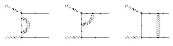
Figure 12: Sample NLO Feynman diagrams contributing to the $\gamma^{*}\gamma\rightarrow q\overline{q}$ amplitude.

Figure 13: Distinct one-loop Feynman diagrams contributing to the $\gamma^{*}\gamma\rightarrow gg$ amplitude. Other contributing diagrams are obtained from these by reversing the direction of the fermion flow in the loops.

The usual renormalization group coefficient is given by

$$\beta_{0}=\frac{11}{3}N_{c}-\frac{2}{3}n_{f}\,.$$ (100)

B.1 Amplitudes

The amplitude $\gamma\gamma\to q\overline{q}$ denoted by $T_{q\overline{q}}$ (examples of contributing Feynman diagrams are depicted in Fig. 12) has the structure already quoted in (LABEL:eq:expT) where

$$T_{q\bar{q}}^{(0)}(u) = \frac{1}{1-u}+\frac{1}{u}\,,$$

$$T_{q\bar{q}}^{(1)}(u) = \frac{-1}{\epsilon}{\cal A}_{col,q\bar{q}}^{(1)}(u)+{\cal A}_{q\bar{q}}^{(1)}(u)\,.$$ (101)

The functions ${\cal A}$ read

$${\cal A}_{col,q\overline{q}}^{(1)}(u) = \frac{1}{1-u}\Big{[}3+2\ln(1-u)\Big{]}+(u\rightarrow 1-u)\,,$$

$${\cal A}_{\;q\overline{q}\;}^{(1)}(u) = \frac{1}{1-u}\left[-9-\frac{1-u}{u}\ln(1-u)+\ln^{2}(1-u)\right]$$ (102)

$$+(u\rightarrow 1-u)\,.$$

In obtaining the above results the projector (91) is employed. The results for the flavor-octet and singlet cases differ only in the flavor factors (see (17) and (44)).

Next, we calculate the amplitude $T_{gg}$ for the subprocess $\gamma^{*}\gamma\rightarrow gg$. The appropriate gluonic projector is the complex conjugate of (94). For the case of the transition form factor we can work in a Breit frame where the momentum of the real photon, $q_{2}$, is proportional to the vector $n$ from Eq. (83), and can therefore be employed in (93). There are 6 one-loop diagrams that contribute to this subprocess amplitude. Three representative diagrams ($G1$, $G2$, $G3$) are shown in Fig. 13. The other three reduce to the first three ones by reversing the direction of the fermion flow in the loop. Moreover, it is easy to see that

$$T_{G2}=-T_{G1}(u\rightarrow 1-u)\,.$$ (103)

Thus, one has only to calculate the contributions from the diagrams $G1$ and $G3$.

The complete unrenormalized NLO contribution is the sum of individual contributions in which, expectedly, the UV singularities cancel. The hard-scattering amplitude $T_{gg}$ has the structure quoted in (LABEL:eq:expT) where $T^{(1)}_{gg}$ is given by

$$T_{gg}^{(1)}(u)=\frac{-1}{\epsilon}{\cal A}_{col,gg}^{(1)}(u)+{\cal A}_{gg}^{(1)}(u)\,.$$ (104)

The functions ${\cal A}$ read

$${\cal A}_{col,gg}^{(1)}(u) = 2\left[\frac{1}{u^{2}}\ln(1-u)-(u\rightarrow 1-u)\right]\,,$$

$${\cal A}_{\>\>gg\>\>}^{(1)}(u) = \frac{2}{u(1-u)}\left[\left(3-\frac{2}{u}\right)\ln(1-u)\right.$$

$$\left.+\frac{1-u}{2u}\ln^{2}(1-u)-(u\rightarrow 1-u)\right]\,.$$

B.2 Kernels

For the calculation of the renormalization matrix $Z$, respective $V^{(1)}$ in (13) we utilize the method proposed in MelicNP01 ; Katz85 of saturating the mesonic state by its valence Fock components (1) which leads to

$$\Phi_{P}^{ur}(u)=-i\tilde{\phi}(u,v)\otimes\left(\begin{array}[c]{c}\langle q\overline{q}_{1};v|P\rangle\\[1.99997pt] \langle gg;v|P\rangle\end{array}\right)\,.$$ (106)

The elements of the matrix $\tilde{\phi}$ are defined as in (84) and (85) with the replacement of $|P\rangle$ by $|q\overline{q}_{1}\rangle$ and $|gg\rangle$. They are thus perturbatively calculable and determine the matrix $Z$.

The calculation of the matrix element $Z_{qq}$ proceeds along the same lines as indicated for the flavor-octet case in Ref. MelicNP01 and the contributing diagrams are displayed there. The respective kernel $V_{qq}$ reads

$$V_{qq}(u,v) = 2\,C_{F}\,\left\{\frac{u}{v}\left[1+\frac{1}{v-u}\right]\Theta(v-u)\right.$$ (109)

$$\left.+\bigg{(}\begin{array}[]{c}u\rightarrow 1-u\\ v\rightarrow 1-v\end{array}\bigg{)}\right\}_{+}\,,$$

where the usual plus distribution is defined as

$$\Big{\{}F(u,v)\Big{\}}_{+}\equiv F(u,v)-\delta(u-v)\int_{0}^{1}dz\,F(z,v)\,.$$ (110)

This result also holds for the flavor-octet case.

Figure 14: LO Feynman diagrams that contribute to $\tilde{\phi}_{qg}$. The crossed circle denotes the vertex of $\langle 0|\overline{\Psi}(-z)\,{\cal C}_{1}\,n/\gamma_{5}/\sqrt{2N_{c}}\Psi(z)$.

We proceed to the evaluation of $Z_{qg}$, or rather $V_{qg}$. According to the definition of the $q\overline{q}_{1}$ distribution amplitude, the matrix element that is of interest here, is given by ($z=[0,z^{-},{\bf 0}_{\perp}]$)

$$\tilde{\phi}_{qg}(u) = \int\frac{dz^{-}}{2\pi}e^{i(2u-1)p\cdot z}$$

$$\times\;\left<0\left|\overline{\Psi}(-z)\;{\cal C}_{1}\;\frac{n/\gamma_{5}}{\sqrt{2N_{c}}}\;\Omega\,\Psi(z)\right|gg\right>\,,$$

The relevant Feynman diagrams for the calculation of $\tilde{\phi}_{qg}$ are depicted in Fig. 14. The $q\overline{q}$ vertex, $\otimes$, is of the form MelicNP01 ; Katz85

$${\cal C}_{1}\frac{\mathbf{1}_{c}}{\sqrt{N_{c}}}\>\frac{n/\gamma_{5}}{2\sqrt{2}}\,\delta(u\,n\cdot p-n\cdot k)\,,$$ (112)

where $k$ represents the momentum of the quark entering the circle. The vertex (112) occurs also in the calculation of the $\tilde{\phi}_{qq}$ where the LO contribution is obtained by contracting the vertex just with the $q\overline{q}$ projector (91) and, hence, one obtains $\tilde{\phi}_{qq}(u,v)=\delta(u-v)$ as it should be (see (13)).

Due to the presence of only one $\gamma_{5}$ matrix, we are confronted with the $\gamma_{5}$ problem, as in the calculation of $T_{q\bar{q}}$. When using the naive $\gamma_{5}$ scheme, in which the $\gamma_{5}$ matrix retains its anticommuting properties in $D$ dimensions, we obtain three different results depending on the position of $\gamma_{5}$ inside the trace:

$$\tilde{\phi}_{qg,D1}(u,v)$$ (113)

$$= -\sqrt{n_{f}C_{F}}\,\frac{\alpha_{s}}{4\pi}\,\left\{\frac{(4\pi)^{2}}{i}\,\left[\mu^{2\epsilon}\int\frac{d^{D}l}{(2\pi)^{D}}\frac{1}{(l^{2}+i\eta)^{2}}\right]\right\}$$

$$\times\left[\frac{u}{v^{2}}\Theta(v-u)-\frac{(1-u)}{(1-v)^{2}}\Theta(u-v)\right.$$

$$\left.+\frac{2\epsilon}{1-\epsilon/2}\delta\left(\frac{u}{v^{2}(1-v)}\Theta(v-u)\right.\right.$$

$$\left.\left.+\frac{(1-u)}{v(1-v)^{2}}\Theta(u-v)\right)\right]\,,$$

where

$$\delta\in\{-(2v-1),-1,1\}\,.$$ (114)

The loop integral can be worked out analytically and we refer to MelicNP01 for the result.

One can easily see that

$$\tilde{\phi}_{qg,D2}(u,v)=-\tilde{\phi}_{qg,D1}(u,1-v)\,,$$ (115)

and finally

$$\tilde{\phi}_{qg}(u,v)=\tilde{\phi}_{qg,D1}(u,v)-\tilde{\phi}_{qg,D1}(u,1-v)\,.$$ (116)

The kernel $V_{qg}$ is a residue of the UV singularity embodied in the loop integral appearing in (113) and, hence, is related to the term multiplying the integral in (113). Since the term proportional to $\delta$ is finite ($\sim\epsilon\,(1/\epsilon)$), it does not contribute to $V_{qg}$. Moreover, since $\tilde{\phi}_{qg}$ being antisymmetric under the replacement of $v$ by $1-v$, is to be convoluted with the matrix element $\left<gg|P\right>$ (see (106)), which has the same symmetry properties as the full gluon distribution amplitude (see (88)), one can replace $\tilde{\phi}_{qg}$ by $\tilde{\phi^{\prime}}_{qg}(u,v)=2\tilde{\phi}_{qg,D1}(u,v)$ in order to obtain a more compact representation of the kernel

$$V_{qg}(u,v)=-2\sqrt{n_{f}C_{F}}\left\{\frac{u}{v^{2}}\Theta(v-u)-\left(\begin{array}[]{c}u\rightarrow 1-u\\ v\rightarrow 1-v\end{array}\right)\right\}\,.$$ (117)

The set of LO evolution kernels is completed by

$$V_{gq}(u,v) = 2\sqrt{n_{f}C_{F}}\left\{\frac{u^{2}}{v}\Theta(v-u)-\left(\begin{array}[]{c}u\rightarrow 1-u\\ v\rightarrow 1-v\end{array}\right)\right\}\,,$$ (120)

$${V}_{gg}(u,v) = 2N_{c}\left\{\frac{u}{v}\left[\left(\frac{\Theta(v-u)}{v-u}\right)_{+}+\frac{2u-1}{v}\Theta(v-u)\right]\right.$$ (124)

$$\left.+\left(\begin{array}[]{c}u\rightarrow 1-u\\ v\rightarrow 1-v\end{array}\right)\right\}+\,\beta_{0}\,\delta(u-v)\,.$$

Since, except of the normalization, there is general agreement in the literature on these kernels, see e.g. Terentev81 ; BaierG81 , we quote them without giving any detail of their calculation. Finally, we comment on an alternative definition of the gluon distribution amplitude which one occasionally encounters in the literature. In that definition the factor $[u(1-u)]^{-1}$ is included in $\phi_{Pg}$ instead in the $gg$ projector (94). The results for $T_{gg}$ (104), (LABEL:eq:agg) will, hence, be multiplied by $u(1-u)$, while the kernels take the form

$$\begin{array}[]{ccc}V_{qg}\rightarrow V_{qg}\;v(1-v)\,,&&\displaystyle V_{gq}\rightarrow\frac{V_{gq}}{u(1-u)}\,,\\[5.69046pt] \lx@intercol\hfil\displaystyle V_{gg}\rightarrow V_{gg}\;\frac{v(1-v)}{u(1-u)}\,.\hfil\lx@intercol\end{array}$$ (125)

The result for the transition form factor, as for any other physical quantity, is, obviously, invariant under the redefinition of the gluon distribution amplitude.

Appendix C Some properties of the evolution kernel

It is easy to verify that the evolution kernels (109) and (117)-(124) satisfy the symmetry relations

$$v\phantom{2}(1-v)\phantom{2}\;V_{qq}(u,v) = u\phantom{2}(1-u)\phantom{2}\;V_{qq}(v,u)\,,$$

$$v^{2}(1-v)^{2}\;V_{gg}(u,v) = u^{2}(1-u)^{2}\>V_{gg}(v,u)\,,$$

$$v^{2}(1-v)^{2}\;V_{qg}(u,v) = u\phantom{2}(1-u)\phantom{2}\>V_{gq}(v,u)\,.$$ (126)

The kernels $V_{ij}$, convoluted with the weighted Gegenbauer polynomials $C_{n}^{m}$ of order $m=3/2,5/2$, result in

$$V_{qq}(u,v)\,\otimes\,v\phantom{2}(1-v)\phantom{2}\,C_{n}^{\,3/2}(2v-1) = \gamma^{qq}_{n}\;u\phantom{2}(1-u)\phantom{2}\,C_{n}^{\,3/2}(2v-1)\,,$$

$$V_{qg}(u,v)\,\otimes\,v^{2}(1-v)^{2}\;C_{n-1}^{5/2}(2v-1) = \gamma^{qg}_{n}\;u\phantom{2}(1-u)\phantom{2}\;C_{n}^{\,3/2}(2v-1)\,,$$

$$V_{gq}(u,v)\,\otimes\,v\phantom{2}(1-v)\phantom{2}\,\,C_{n}^{3/2}(2v-1) = \gamma^{gq}_{n}\;u^{2}(1-u)^{2}\,C_{n-1}^{5/2}(2v-1)\,,$$

$$V_{gg}(u,v)\,\otimes\,v^{2}(1-v)^{2}\;C_{n-1}^{5/2}(2v-1) = \gamma^{gg}_{n}\;u^{2}(1-u)^{2}\,\,C_{n-1}^{5/2}(2v-1)\,.$$ (127)

The factors on the right hand side of (127) multiplying the Gegenbauer polynomials are the anomalous dimensions. The results quoted for them in (LABEL:eq:andim) can be read off from (127) (for a detailed discussion see BaierG81 ). Finally, we mention that the off-diagonal anomalous dimensions in (LABEL:eq:andim) satisfy the relation

$$\frac{\gamma_{n}^{qg}}{\gamma_{n}^{gq}}=\frac{N_{n-1}^{\,5/2}}{N_{n}^{\,3/2}}\,,$$ (128)

where

$$N_{n}^{3/2} = \frac{(n+1)(n+2)}{4(2n+3)}\,,$$ (129)

$$N_{n-1}^{5/2} = \frac{n(n+3)}{36}N_{n}^{3/2}\,,\,$$ (130)

represent the normalization constants of the corresponding Gegenbauer polynomials

$$\int_{0}^{1}du\,u(1-u)\,C_{n}^{\,3/2}(2u-1)C_{m}^{3/2}(2u-1) = N_{n}^{\,3/2}\,\delta_{nm}\,,$$

$$\int_{0}^{1}du\,u^{2}(1-u)^{2}\,C_{n}^{\,5/2}(2u-1)C_{m}^{5/2}(2u-1) = N_{n}^{\,5/2}\,\delta_{nm}\,.$$

Throughout the paper we investigate only the LO behavior of the evolution kernels and corresponding anomalous dimensions. Beyond leading order, the relations corresponding to (127) and (128) get modified due to mixing of conformal operators starting at NLO (see, for example, BelitskyMS99 ).

References

- (1) G. P. Lepage and S. J. Brodsky, Phys. Lett. B 87, 359 (1979), A. V. Efremov and A. V. Radyushkin, Phys. Lett. B 94, 245 (1980); A. Duncan and A. H. Mueller, Phys. Rev. D 21, 1636 (1980).
- (2) G. P. Lepage and S. J. Brodsky, Phys. Rev. D 22, 2157 (1980).
- (3) T. Feldmann, Int. J. Mod. Phys. A 15, 159 (2000) [hep-ph/9907491]; T. Feldmann and P. Kroll, Phys. Scripta T99, 13 (2002) [hep-ph/0201044].
- (4) M. V. Terentev, Sov. J. Nucl. Phys. 33, 911 (1981) [Yad. Fiz. 33, 1692 (1981)].
- (5) T. Ohrndorf, Nucl. Phys. B 186, 153 (1981).
- (6) M. A. Shifman and M. I. Vysotsky, Nucl. Phys. B 186, 475 (1981).
- (7) V. N. Baier and A. G. Grozin, Nucl. Phys. B 192, 476 (1981).
- (8) V. N. Baier and A. G. Grozin, Fiz. Elem. Chast. Atom. Yadra 16, 5 (1985) [Sov. J. Part. Nucl. 16, 1 (1985) ].
- (9) J. Blümlein, B. Geyer and D. Robaschik, in *Hamburg/Zeuthen 1997, Deep inelastic scattering off polarized targets, Physics with polarized protons at HERA* 196-209, [hep-ph/9711405].
- (10) A. V. Belitsky and D. Müller, Nucl. Phys. B 527, 207 (1998) [hep-ph/9802411]; A. V. Belitsky, D. Müller, L. Niedermeier and A. Schäfer, Nucl. Phys. B 546, 279 (1999) [hep-ph/9810275].
- (11) A. V. Belitsky and D. Müller, Nucl. Phys. B 537, 397 (1999) [hep-ph/9804379].
- (12) B. Melić, B. Nižić and K. Passek, Phys. Rev. D 65, 053020 (2002) [hep-ph/0107295].
- (13) M. Diehl, P. Kroll and C. Vogt, Eur. Phys. J. C 22, 439 (2001) [hep-ph/0108220].
- (14) J. Gronberg et al. [CLEO Collaboration], Phys. Rev. D 57, 33 (1998) [hep-ex/9707031].
- (15) M. Acciarri et al. [L3 Collaboration], Phys. Lett. B 418, 399 (1998).
- (16) T. Feldmann, P. Kroll and B. Stech, Phys. Rev. D 58, 114006 (1998) [hep-ph/9802409] and Phys. Lett. B 449, 339 (1999) [hep-ph/9812269].
- (17) J. Bolz, P. Kroll and G. A. Schuler, Phys. Lett. B 392, 198 (1997) [hep-ph/9610265], Eur. Phys. J. C 2, 705 (1998) [hep-ph/9704378].
- (18) F. del Aguila and M. K. Chase, Nucl. Phys. B 193, 517 (1981); E. Braaten, Phys. Rev. D 28, 524 (1983); E. P. Kadantseva, S. V. Mikhailov and A. V. Radyushkin, Yad. Fiz. 44, 507 (1986) [Sov. J. Nucl. Phys. 44, 326 (1986)].
- (19) S. V. Mikhailov and A. V. Radyushkin, Nucl. Phys. B 254, 89 (1985).
- (20) M. A. Ahmed and G. G. Ross, Nucl. Phys. B 111, 441 (1976).
- (21) D. Müller, Phys. Rev. D 51, 3855 (1995) [hep-ph/9411338].
- (22) P. Kroll and M. Raulfs, Phys. Lett. B 387, 848 (1996) [hep-ph/9605264].
- (23) H. Leutwyler, Nucl. Phys. Proc. Suppl. 64, 223 (1998) [hep-ph/9709408]; R. Kaiser and H. Leutwyler, Eur. Phys. J. C 17, 623 (2000) [hep-ph/0007101].
- (24) T. Feldmann and P. Kroll, Eur. Phys. J. C 5, 327 (1998) [hep-ph/9711231].
- (25) R. Jakob, P. Kroll and M. Raulfs, J. Phys. G 22, 45 (1996) [hep-ph/9410304].
- (26) I. V. Musatov and A. V. Radyushkin, Phys. Rev. D 56, 2713 (1997) [hep-ph/9702443].
- (27) B. Melić, B. Nižić and K. Passek, hep-ph/0107311.
- (28) C. Caso et al. [Particle Data Group Collaboration], Eur. Phys. J. C 3, 1 (1998).
- (29) M. Acciarri et al. [L3 Collaboration], Phys. Lett. B 461, 155 (1999) [hep-ex/9909008].
- (30) T. Feldmann and P. Kroll, Phys. Lett. B 413, 410 (1997) [hep-ph/9709203].
- (31) J. Botts and G. Sterman, Nucl. Phys. B 325, 62 (1989).
- (32) A. V. Radyushkin, Phys. Lett. B 385, 333 (1996) [hep-ph/9605431].
- (33) J. C. Collins, L. Frankfurt and M. Strikman, Phys. Rev. D 56, 2982 (1997) [hep-ph/9611433].
- (34) D. Müller, D. Robaschik, B. Geyer, F. M. Dittes and J. Hořejši, Fortsch. Phys. 42, 101 (1994) [hep-ph/9812448]; X. D. Ji, Phys. Rev. D 55, 7114 (1997) [hep-ph/9609381]; A. V. Radyushkin, Phys. Rev. D 56, 5524 (1997) [hep-ph/9704207].
- (35) L. Mankiewicz, G. Piller and T. Weigl, Eur. Phys. J. C 5, 119 (1998) [hep-ph/9711227]; M. Vanderhaeghen, P. A. Guichon and M. Guidal, Phys. Rev. D 60, 094017 (1999) [hep-ph/9905372]; M. I. Eides, L. L. Frankfurt and M. I. Strikman, Phys. Rev. D 59, 114025 (1999) [hep-ph/9809277].
- (36) H. W. Huang and P. Kroll, Eur. Phys. J. C 17, 423 (2000) [hep-ph/0005318].
- (37) M. Diehl, T. Feldmann, R. Jakob and P. Kroll, Eur. Phys. J. C 8, 409 (1999) [hep-ph/9811253].
- (38) L. Mankiewicz and G. Piller, Phys. Rev. D 61, 074013 (2000) [hep-ph/9905287].
- (39) T. Muta and M. Z. Yang, Phys. Rev. D 61, 054007 (2000) [hep-ph/9909484].
- (40) A. Ali and A. Y. Parkhomenko, Phys. Rev. D 65, 074020 (2002) [hep-ph/0012212].
- (41) V. N. Baier and A. G. Grozin, Z. Phys. C 29, 161 (1985).
- (42) M. Beneke, hep-ph/0207228.
- (43) A. B. Wakely and C. E. Carlson, Phys. Rev. D 45, 338 (1992).
- (44) S. J. Brodsky, P. Damgaard, Y. Frishman and G. P. Lepage, Phys. Rev. D 33, 1881 (1986).
- (45) G. R. Katz, Phys. Rev. D 31, 652 (1985).
- (46) V. L. Chernyak and A. R. Zhitnitsky, Phys. Rept. 112, 173 (1984).
- (47) S. J. Brodsky, H. C. Pauli and S. S. Pinsky, Phys. Rept. 301, 299 (1998) [hep-ph/9705477].
- (48) M. Diehl, T. Feldmann, R. Jakob and P. Kroll, Nucl. Phys. B 596, 33 (2001) [Erratum-ibid. B 605, 647 (2001)] [hep-ph/0009255].
- (49) J. B. Kogut and D. E. Soper, Phys. Rev. D 1, 2901 (1970).
- (50) A. V. Belitsky and D. Müller, Phys. Lett. B 417, 129 (1998) [hep-ph/9709379]; L. Mankiewicz, G. Piller, E. Stein, M. Vanttinen and T. Weigl, Phys. Lett. B 425, 186 (1998) [hep-ph/9712251]; X. D. Ji and J. Osborne, Phys. Rev. D 58, 094018 (1998) [hep-ph/9801260].
- (51) A. V. Belitsky, D. Müller and A. Schäfer, Phys. Lett. B 450, 126 (1999) [hep-ph/9811484].