hep-ph/0209372
                                                                         September 2002

Higgs physics at a high luminosity $\rm e^{+}e^{-}$ linear collider
André Sopczak
Lancaster University, UK

Abstract

Abstract

Since the TESLA Technical Design Report (TDR) was published in 2001, the physics programme of an electron-positron linear collider (LC) has been further developed and a wide consensus has been reached on the physics case and the need for a high luminosity LC with center-of-mass energy up to about 1 TeV as the next worldwide high-energy physics project. The study of the Higgs boson properties represents a significant part of this physics programme. New studies demonstrate that a LC providing 1000 fb^-1 of data at center-of-mass energies of at least 500 GeV, is an excellent Higgs boson analyzer for a wide range of masses. A summary of preliminary results of these studies and their implications for identifying the nature of the Higgs sector and for constraining the parameter space of extended models is given. The focus is on recent developments and the relation to the LHC is addressed.

1 INTRODUCTION

A linear collider of at least 500 GeV and a total luminosity of at least 1000 fb^-1 has much potential for studying Higgs bosons and understanding the electroweak symmetry breaking and mass generation. Already at the CERN $\rm e^{+}e^{-}$ collider, LEP, enormous progress for Higgs boson searches has been made. At LEP-1 [1] many search channels were almost background free and also at LEP-2 [2] the sensitivity exceeded expectations, leading to a Standard Model (SM) Higgs boson mass limit of 114 GeV at 95% CL. A small indication at LEP of a 115 GeV SM Higgs boson could also be interpreted in extended models [3].

During the last 10 years, LC studies have evolved from discovery studies to studies of precision measurements. Recent milestones were set with the TESLA TDR [4], the Snowmass Study [5] and the international workshop on LC in Korea [6].

This review will focus on new results and developments. First, I will address the SM physics and discuss how precisely a future LC can determine the Higgs boson production mechanism. Indirect and direct branching ratio measurements are reviewed. Then the characterization of the Higgs boson potential, which will contribute to establishing the underlying mechanism of mass generation, is addressed. Higgs bosons could also be produced via Higgs-strahlung off top quarks. In the general two Higgs doublet model (2HDM) charged Higgs bosons are prominent. Various methods to determine the ratio of the vacuum expectation values of the two doublets, $\tan\beta$, are discussed. In the framework of the Minimal Supersymmetric extension of the SM (MSSM) or beyond, invisibly decaying Higgs bosons could be produced and their properties measured. Furthermore, the measurement of the Higgs boson parity is discussed as well as important possibilities to distinguish Higgs boson models. For several LC studies the relation to the LHC potential is addressed. The importance of beam polarization and the option of a $\gamma\gamma$ collider are reviewed elsewhere [7, 8]. Future LC Higgs studies will concentrate on more detailed detector simulations reflecting the progress in detector technologies, the second phase of a LC with center-of-mass energies up to 1 TeV for TESLA, and new theoretical developments, such as extra dimensions.

2 STANDARD MODEL PHYSICS

2.1 Higgs boson production mechanism

The expected SM Higgs production rate has a very large significance over the background ($\sigma\equiv N_{\rm sig}/\sqrt{N_{\rm bg}}$) [9]. More than $100\sigma$ is obtainable in the $\rm H\rightarrow b\bar{b}$ decay channel. For heavier Higgs bosons, the WW decay mode takes over. In relation to the LHC [10], a LC has a much larger sensitivity in the lower mass range, while the LHC can probe heavier Higgs bosons. At about 115 GeV mass, the LEP sensitivity reduces from about $4\sigma$ to $2\sigma$ [2]. Figure 1 (from [9]) shows the SM Higgs boson detection significance.

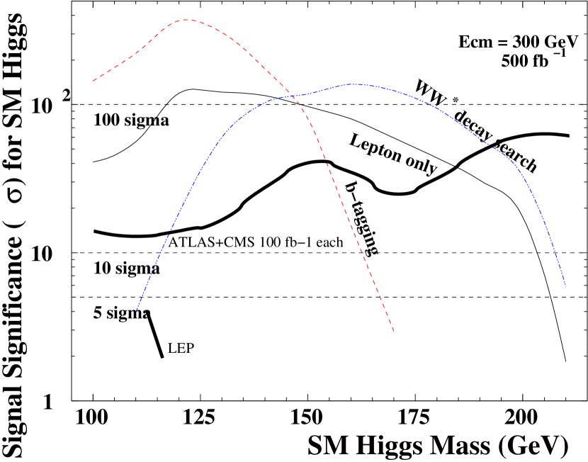
Figure 1: SM Higgs boson signal significance.

The sensitivity to the general production cross section has been studied [9]. The expected SM production cross section is much larger than the $5\sigma$ sensitivity to the cross section over a wide mass range. For lower masses the Higgs boson decay mode into a pair of b-quarks gives the largest sensitivity. Figure 2 (from [9]) shows also the cross section sensitivity for any Higgs boson decay mode, where the Higgs boson mass is reconstructed as the recoiling mass to the Z decay products. Even for models beyond the SM, the sensitivity to the cross section is much better than the expected minimal production cross section.

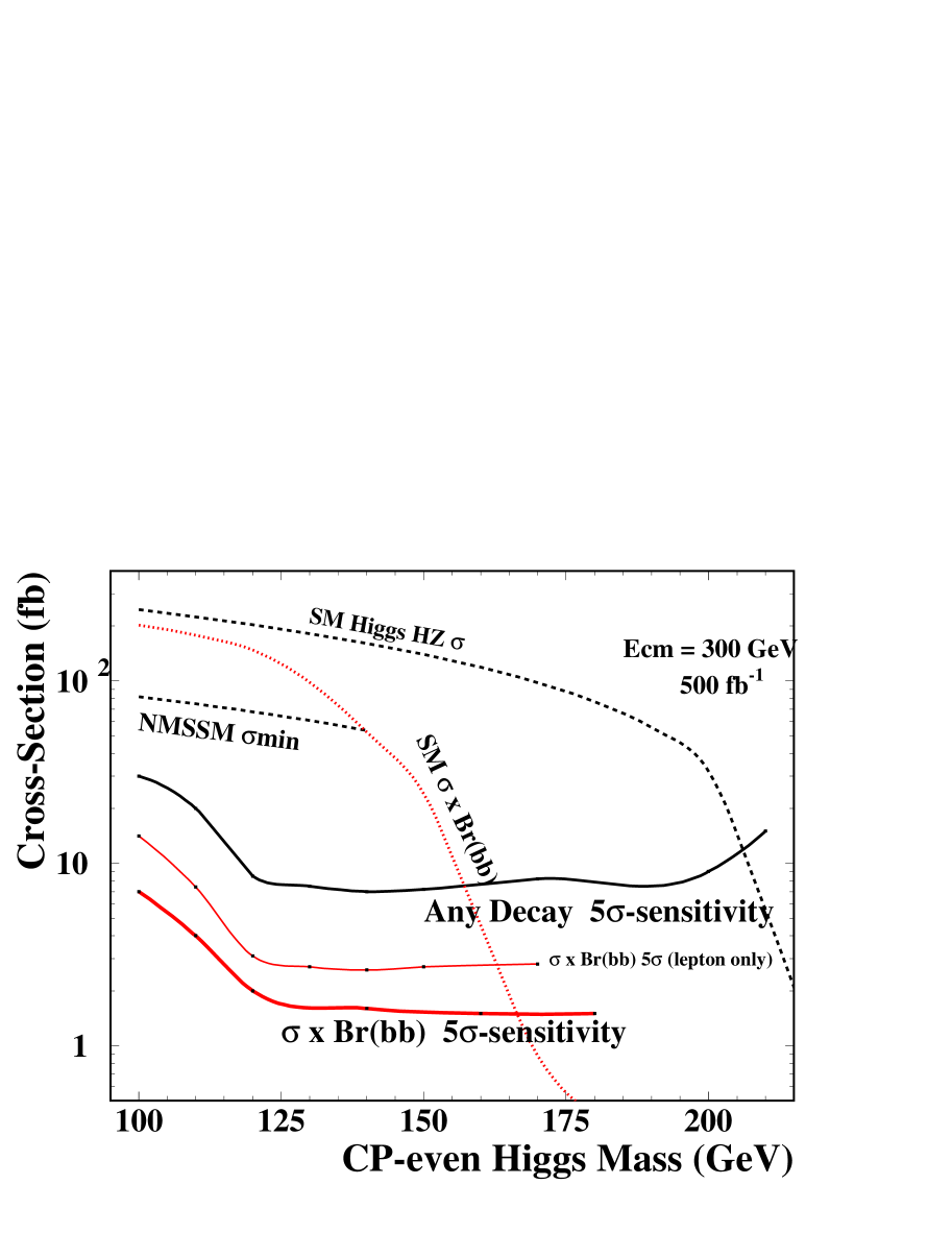
Figure 2: Expected production cross sections (dashed lines) and simulated experimental sensitivities (solid lines).

The Higgs boson will be produced via Higgs-strahlung and WW fusion by the two processes

$$\rm e^{+}e^{-}\rightarrow HZ\rightarrow H\nu\bar{\nu}\rightarrow b\bar{b}\nu\bar{\nu}~{}~{}~{}and$$

$$\rm e^{+}e^{-}\rightarrow WW\nu\bar{\nu}\rightarrow\nu\bar{\nu}H\rightarrow\nu\bar{\nu}b\bar{b}.$$

These production mechanisms can be distinguished by fitting the missing mass distribution [11] as shown in Fig. 3 (from [12]). Higgs-strahlung gives a shape like the dashed line, while Higgs boson fusion is represented by the dotted line. Their sum is given by the solid line and the simulated data is shown with error bars.

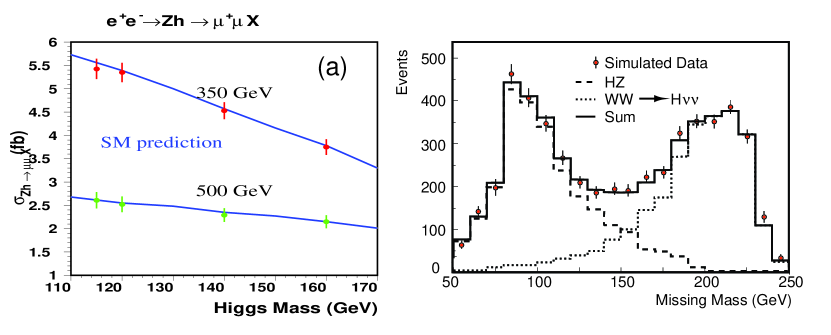
Figure 3: Expected missing mass distributions for Higgs-strahlung and WW fusion. Their sum is shown in comparison with simulated data.

2.2 Indirect and direct branching ratio measurements

A LC will perform very high precision measurements of the Higgs boson branching fractions. The underlying production process is the Higgs-strahlung,

$$\rm e^{+}e^{-}\rightarrow HZ\rightarrow H\ell^{+}\ell^{-},$$

where the associated Z boson decays into a lepton pair. Two methods are discussed to determine the Higgs boson branching ratio.

In the indirect method, the inclusive production cross section as the product of the Higgs boson production cross section and the branching fraction of the Z into leptons is determined:

$$\sigma_{\rm inc}=\sigma_{\rm HZ}BR(\rm Z\rightarrow\ell^{+}\ell^{-}).$$

This measurement is independent of the Higgs boson decay mode. The mass recoiling to the lepton pair corresponds to the Higgs boson mass. An individual Higgs boson decay cross section is measured, which is the product of the Higgs boson production cross section and the Higgs and Z boson decay branching fractions:

$$\sigma({\rm X})=\sigma_{\rm HZ}BR({\rm Z\rightarrow Y})BR({\rm H\rightarrow X}).$$

By taking the ratio of both cross sections the Higgs branching ratio can be determined, since the LEP experiments measured the Z decay branching fractions with high precision.

The Higgs boson branching ratios can also be determined directly from the HZ($\rm Z\rightarrow\ell^{+}\ell^{-}$) event sample [13]. The Higgs boson mass is reconstructed as the recoiling mass of the lepton pair:

$$m_{\rm H}=m_{\ell^{+}\ell^{-}}^{\rm recoil}.$$

The simulation was performed for $\sqrt{s}=360$ GeV and ${\cal L}=500$ fb^-1 [13]. Figure 4 shows this event sample which is enriched with Higgs bosons by the indicated cuts. The expected signal distribution is given with error bars and the expected background as a histogram. In this event sample individual Higgs boson decay modes are selected. The resulting precision on the Higgs boson decay branching ratios as well as a preliminary combination of both methods [13] are listed in Table 1.

Table 1: Expected precision on branching ratios (in %) for a 120 GeV Higgs boson from the direct method and a preliminary combination with the indirect method.

Decay	SM $BR$	$\Delta BR_{\rm d}/BR_{\rm d}$	$\Delta BR_{\rm c}/BR_{\rm c}$
bb	68	1.9	1.5
$\tau\tau$	6.9	7.1	4.1
cc	3.1	8.1	5.8
gluons	7.0	4.8	3.6
$\gamma\gamma$	0.22	35	21
WW⋆	13	3.6	2.7

In relation to the LHC, a LC will achieve a much higher precision and will cover all decay modes. This would also allow precision testing of the fundamental relation between the Yukawa coupling and the Higgs boson mass:

$$g_{\rm Hff}\propto m_{\rm f}.\vspace*{-3mm}$$

Figure 4: Simulated events for a direct determination of the Higgs boson decay branching ratios.

2.3 Mass and width determination

Further properties of the Higgs boson, like its mass and decay width, can be determined with high precision. A study of a 240 GeV SM Higgs boson in the reactions

$$\rm e^{+}e^{-}\rightarrow HZ\rightarrow WWZ~{}~{}~{}and$$

$$\rm e^{+}e^{-}\rightarrow HZ\rightarrow ZZZ$$

has been performed [14]. A very clear signal with only a few background events is expected. Figure 5 shows the expected signal and background mass distribution. The fit of the reconstructed mass peak leads to a mass resolution of 0.08% and an 11% error on the total decay width.

This result is shown in comparison with results from other reactions on the determination of the Higgs boson mass [15]. Figure 6 shows results from a CMS study (curve 1) where the Higgs boson decays into a pair of Z bosons, which subsequently decay into muon pairs. The sensitivity reduction near 160 GeV is due to dominant decays into W pairs. The curves 2 and 3 show extrapolated results according to the cross section and branching ratio expectations for a LC operation at 350 and 500 GeV. In the low mass region indirect methods can be applied (curve 4) and for very low masses, the LHC has high sensitivity in the photon decay mode.

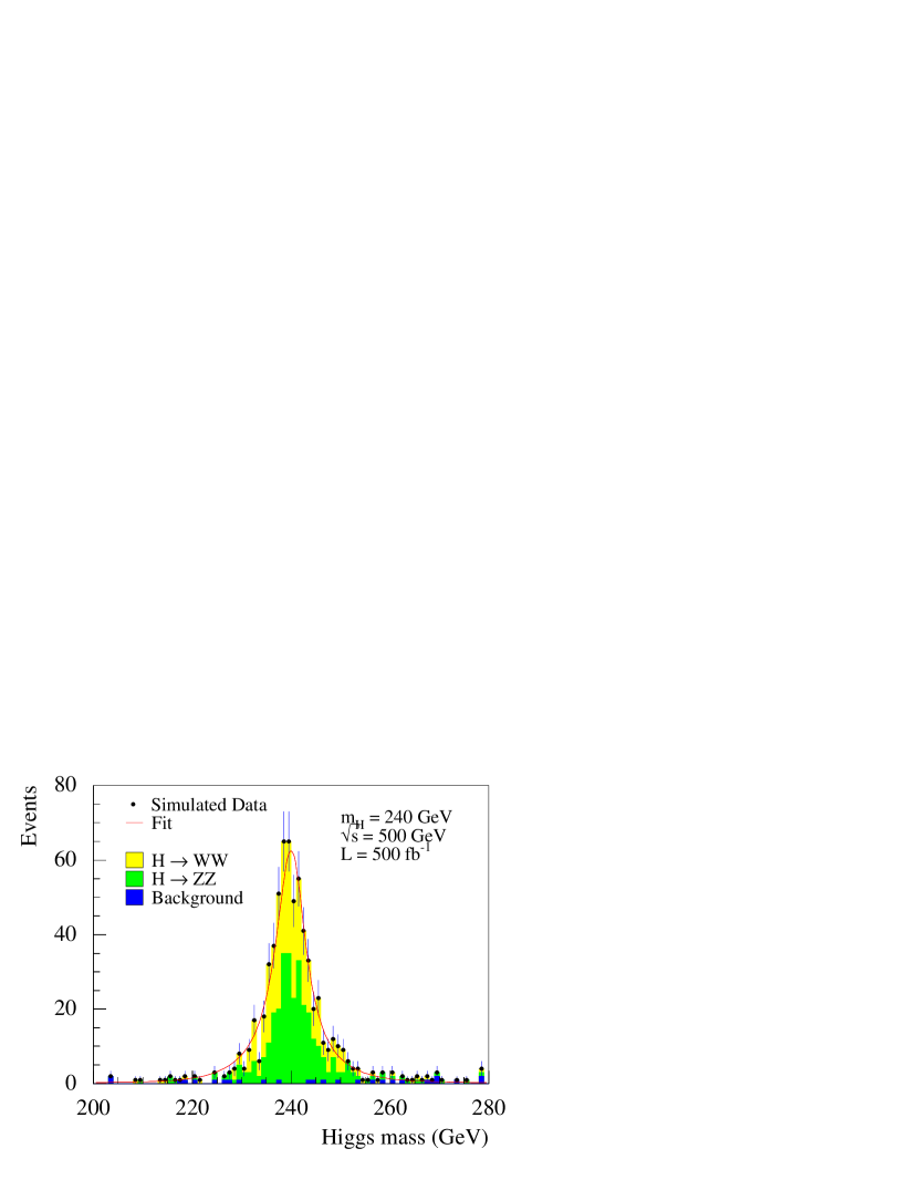
Figure 5: Mass and width determination.

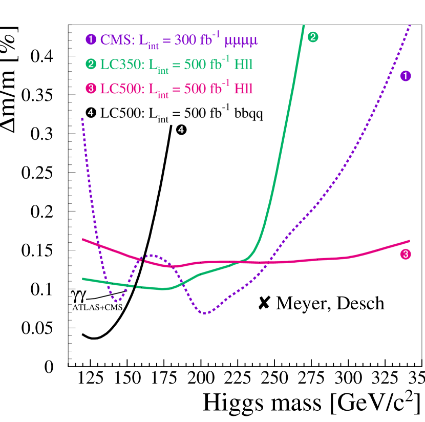
Figure 6: Comparison of different methods to determine the Higgs boson mass.

2.4 Characterization of the Higgs boson potential

A LC will be able to measure fundamental properties of the Higgs boson potential. The Higgs boson can decay into a pair of Higgs bosons:

$$\rm e^{+}e^{-}\rightarrow HZ\rightarrow HHZ.$$

Figure 7 illustrates this Higgs boson production reaction.

Figure 7: Higgs boson self-coupling reaction.

The self-coupling interaction can probe the shape of the Higgs boson potential through the relation

$$g_{\rm HHH}=3m_{\rm H}^{2}/2v,$$

where $v=246$ GeV. A sensitivity of $\Delta g/g=29$% was obtained for $m_{\rm H}=120$ GeV, $\sqrt{s}=800$ GeV and ${\cal L}=1000$ fb^-1 [16, 17]. Figure 8 shows the precision on the Higgs boson self-coupling where the lines indicate $g_{\rm HHH}/g_{\rm HHH}^{\rm SM}=1.25,~{}1.00,~{}0.75,~{}0.50$. Higher sensitivity of $\Delta g/g=7$% could be reached for a LC with $\sqrt{s}=3$ TeV and ${\cal L}=5000$ fb^-1 as shown in Fig. 9.

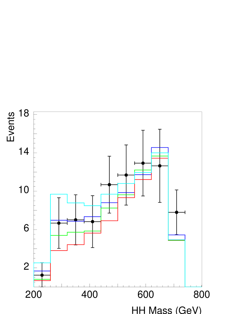
Figure 8: Reconstructed invariant mass of the HH pairs.

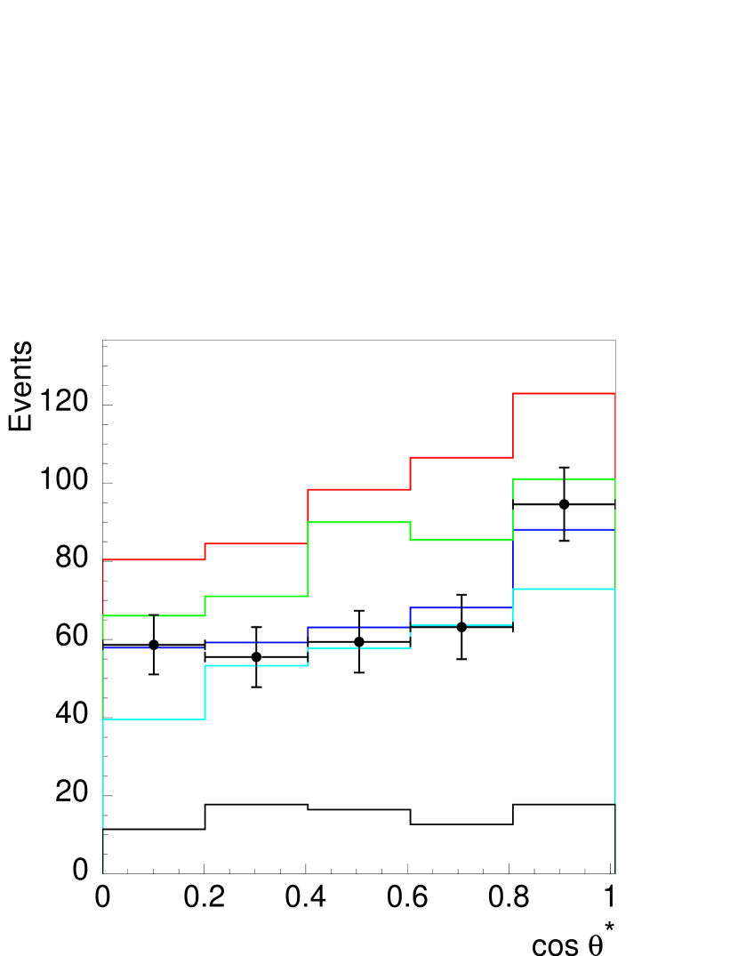
Figure 9: Reconstructed angle between the H and HH directions.

2.5 Higgs-strahlung from top quarks

Owing to the strong coupling of Higgs bosons to top quarks, the radiation of Higgs boson off top quarks is a possible production mechanism (Fig. 10). The decay modes involving a pair of b quarks and W bosons were studied in the reactions [18]

$$\rm e^{+}e^{-}\rightarrow t\bar{t}H\rightarrow t\bar{t}b\bar{b}~{}~{}~{}and$$

$$\rm e^{+}e^{-}\rightarrow t\bar{t}H\rightarrow t\bar{t}WW.$$

A challenge is the precision determination of the background to a level of 5% uncertainty, leading to

$$\Delta g_{\rm ttH}/g_{\rm ttH}=7.5\%~{}{\rm to}~{}20\%.$$

Figure 11 shows the resulting precision for the $\rm b\bar{b}$ and WW decay modes, as well as their statistical combination as a function of the SM Higgs boson mass. In addition, a previous study at 120 GeV with slightly higher sensitivity is indicated [19].

Figure 10: $\rm t\bar{t}H$ production process.

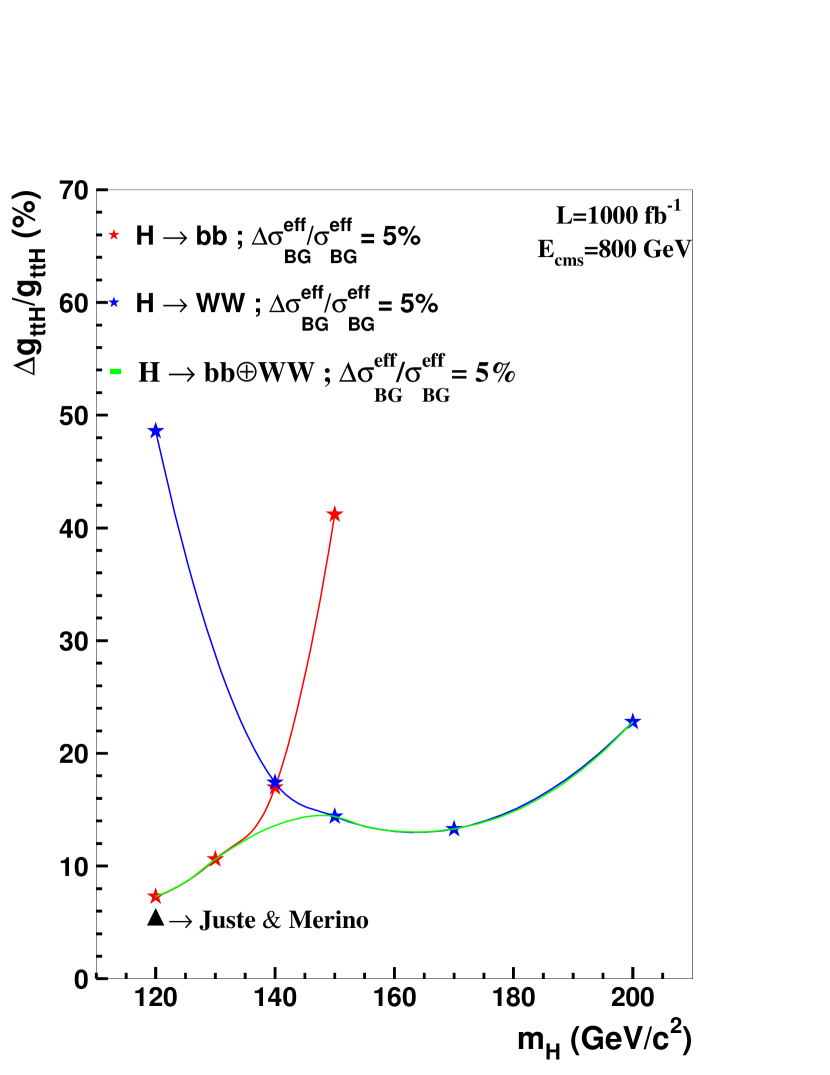
Figure 11: Expected precision on the Yukawa coupling $g_{\rm ttH}$.

3 BEYOND THE STANDARD MODEL

3.1 Charged Higgs bosons

The discovery of charged Higgs bosons would immediately prove that physics beyond the SM exists. The reaction

$$\rm e^{+}e^{-}\rightarrow Z\rightarrow H^{+}H^{-}\rightarrow t\bar{b}\bar{t}b$$

can be observed at a LC [20] and recent high-luminosity simulations [21] show that the production cross section times branching ratio can be measured very precisely:

$$\Delta(\sigma BR({\rm H^{+}\rightarrow t\bar{b}}))/\sigma BR({\rm H^{+}\rightarrow t\bar{b}})=8.8\%$$

for $m_{\rm H^{\pm}}=300$ GeV, $\sqrt{s}=800$ GeV and ${\cal L}=1000$ fb^-1. A detailed reconstruction of the entire decay chain, as illustrated in Fig. 12, is possible. Figure 13 shows a clear expected charged Higgs boson signal and small background.

Figure 12: Charged Higgs boson production and decay.

Figure 13: Expected charged Higgs boson signal and background.

3.2 Determination of $\tan\beta$

The ratio of the vacuum expectation values $\tan\beta$ can be measured with several methods. The pseudoscalar Higgs boson, A, could be produced via radiation off a pair of b-quarks:

$$\rm e^{+}e^{-}\rightarrow b\bar{b}\rightarrow b\bar{b}A\rightarrow b\bar{b}b\bar{b}.$$

Figure 14 illustrates the production process. The $\rm b\bar{b}A$ coupling is proportional to $\tan\beta$ and thus the expected production rate is proportional to $\tan^{2}\beta$. A precision better than 10% can be achieved for a Higgs boson mass of 100 GeV and large $\tan\beta$ values [22]. The sensitivity decreases with increasing Higgs boson masses and decreasing $\tan\beta$ values as shown in Fig. 15. This study assumes a luminosity of 2000 fb^-1, corresponding to several years of data taking.

Figure 14: bbA production to determine the value of $\tan\beta$.

Figure 15: 2HDM $\tan\beta$ determination.

There are further methods to determine $\tan\beta$:

• The $\rm b\bar{b}\bar{b}b$ rate from the pair-production of the heavier scalar in association with the pseudoscalar Higgs boson,

  $$\rm e^{+}e^{-}\rightarrow HA\rightarrow b\bar{b}b\bar{b},$$

  can be exploited. While the HA production rate is almost independent of $\tan\beta$ the sensitivity is achieved owing to the variation of the decay branching ratios with $\tan\beta$.

• The value of $\tan\beta$ can also be determined from the H and A decay widths, which can be obtained from the previously described reaction.

• The pair-production rate and total decay width of charged Higgs bosons can contribute to the determination of $\tan\beta$. Charged Higgs boson production can also be used at the LHC to measure $\tan\beta$ [23].

The results from the methods involving the neutral Higgs bosons are summarized in Fig. 16 for the MSSM. As the H and A decay rates depend on the MSSM parameters, two cases are considered. In case (I) heavy Supersymmetric particles are expected, while in case (II) the Higgs bosons could decay into light Supersymmetric particles.

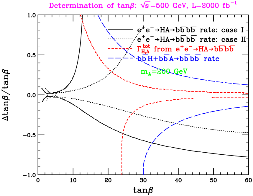
Figure 16: MSSM $\tan\beta$ determination.

3.3 Invisible Higgs boson decays

Among other possibilities, invisible Higgs boson decays could occur from the reaction involving neutralinos:

$$\rm e^{+}e^{-}\rightarrow ZH\rightarrow Z\tilde{\chi}^{0}\tilde{\chi}^{0}.$$

In this case the Higgs boson mass can be reconstructed from the recoiling mass of the visible decay products:

$$m_{\rm H}=m_{\rm Z}^{\rm recoil}.$$

At LEP all Z decay modes involving charged fermions contributed to the search, while in a recent LC study [24] so far only the hadronic decay mode $\rm Z\rightarrow q\bar{q}$ has been investigated. This study for $\sqrt{s}=350$ GeV and ${\cal L}=500$ fb^-1 gives higher sensitivity compared to indirect methods ($1-$ sum of visible H decay modes). For Higgs boson branching ratios $BR_{\rm i}$ into invisible decay products larger than 20% and a SM Higgs boson production rate,

$$\Delta BR_{\rm i}/BR_{\rm i}<4\%$$

can be achieved. Figure 17 shows the resulting sensitivities as a function of the branching ratio into invisible decays.

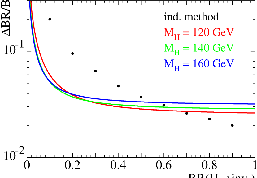
Figure 17: Expected precision on the invisible Higgs boson branching fraction. The dots represent the indirect method.

3.4 Higgs boson parity

After the discovery of one or several Higgs bosons, it is very important to determine the parity of the Higgs bosons and distinguish a CP-even H boson from a CP-odd A boson. This could be achieved by investigating the Higgs boson decay properties into $\tau$-leptons. The subsequent decay of the $\tau$’s into $\rho$’s and pions through the reaction

$$\rm H/A\rightarrow\tau^{+}\tau^{-}\rightarrow\rho^{+}\bar{\nu}_{\tau}\rho^{-}\nu_{\tau}\rightarrow\pi^{+}\pi^{0}\bar{\nu}_{\tau}\pi^{-}\pi^{0}\nu_{\tau}$$

is studied [25].

The $\rho^{+}\rho^{-}$ acoplanarity angle is defined by the planes of the pions in the rest frame of the $\rho$’s (Fig. 18). The acoplanarity angle distribution clearly distinguishes the different parity states. Figure 19 shows the acoplanarity angle before detector effects are included, and Fig. 20 after a preliminary detector simulation. The thick line is the expectation for scalar Higgs bosons and the thin line for pseudoscalar Higgs bosons.

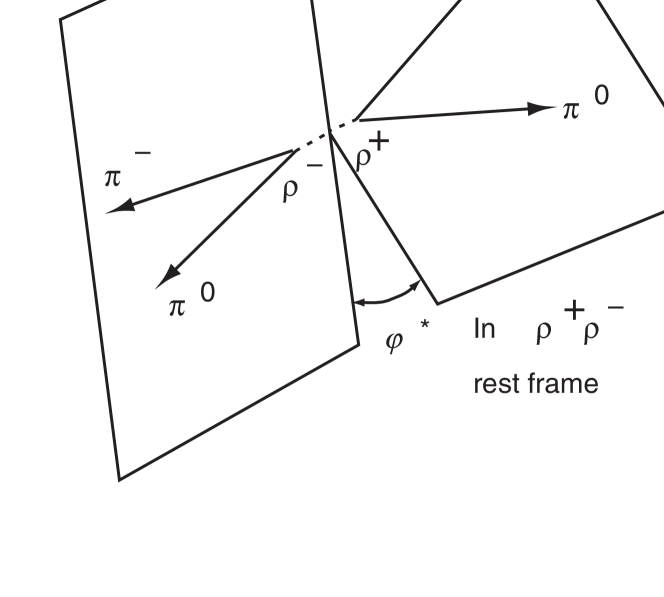
Figure 18: Acoplanarity angle definition.

Figure 19: Higgs boson parity determination before detector simulation.

Figure 20: Higgs boson parity determination after a preliminary detector simulation.

3.5 Distinction of Higgs boson models

The distinction of Higgs boson models is very important and could be based on precision branching ratio measurements. The ratio of the Higgs boson decay rates into b-quarks and $\tau$-leptons is defined by

$$R\equiv BR({\rm H/A\rightarrow b\bar{b})}/BR({\rm H/A\rightarrow\tau^{+}\tau^{-}}).$$

The normalized value of $R$ to the SM expectation can be used to distinguish a general 2HDM from the MSSM. Large deviations from $R=1$ are expected in the MSSM for several MSSM parameter combinations [26] as shown in Fig. 21. In relation to the LHC, where models can only be distinguished for $\tan\beta>25$, a LC covers the entire $\tan\beta$ range.

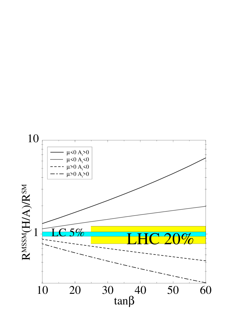
Figure 21: Distinction of Higgs boson models from precision Higgs boson decay branching ratio determinations.

Important predictions on the pseudoscalar Higgs boson mass can be made from the precision measurements of the scalar Higgs boson branching ratios:

$$BR({\rm H\rightarrow b\bar{b}})/BR({\rm H\rightarrow WW}).$$

A LC obtains a precision normalized to the SM expectation of less than $3.5$%, while the expected precision at the LHC is less than $20$%. For a 400 GeV pseudoscalar Higgs boson A, its mass can be predicted at a LC with an error of about 50 GeV, while at the LHC only a lower mass limit can be set [27]. Figure 22 shows the sensitivity on the prediction of the A boson mass at the LHC and a LC for a wide range of A masses.

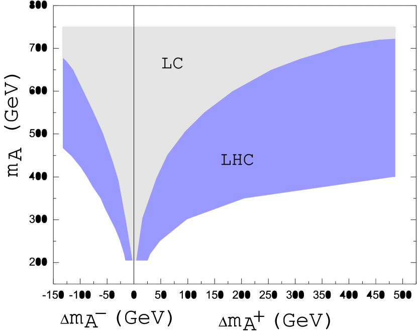
Figure 22: Comparison of LHC and LC A mass predictions from precision scalar Higgs boson decay branching ratio determinations.

Beyond the MSSM, the Higgs boson particle spectrum is enriched for example in the framework of the Non-Minimal Supersymmetric extension of the SM (NMSSM) [28] where an extra Higgs boson singlet $\lambda NH_{1}H_{2}$ is present. Such a model could be distinguished from the MSSM by precision measurements of the Higgs boson masses and comparison with the predictions. Moreover, additional light neutral Higgs bosons may be observed and the mass sum rules are modified, leading, for example, to a reduced mass of the charged Higgs boson.

4 CONCLUSIONS

• After a first discovery and initial precision measurements in some decay modes at the Tevatron or the LHC, already in the first phase of a LC, many Higgs boson decay modes will be measured with very high precision.

• The precise LC data will allow the determination of the nature of the Higgs sector. Models like the SM, the general 2HDM, the MSSM and the NMSSM will be distinguished for a wide range of parameters.

• The underlying mechanism of symmetry breaking and mass generation will be tested.

• Like for the top quark (LEP mass prediction, Tevatron observation), important consistencies of the model can be probed with combined LC and LHC physics.

• After 10 years of preparatory studies the LC has a solid case and the high-energy physics community is prepared to answer fundamental questions over the coming decades.

References

- [1] A. Sopczak, Phys. Rep. 359 (2002) 169.
- [2] LEP Higgs Working Group, July 2002.
- [3] A. Sopczak, ABS684, ICHEP02, Amsterdam, 2002.
- [4] TESLA TDR, DESY (2001).
- [5] American Physical Society study on the future of particle physics, Snowmass, USA, July 2001.
- [6] Int. Workshop on LC, Jeju, Korea, Aug. 2002.
- [7] G. Moortgat-Pick, ABS23, ICHEP02, Amsterdam, 2002.
- [8] S. Soldner-Rembold, ABS770, ICHEP02, Amsterdam, 2002.
- [9] S. Yamashita et. al., hep-ph/0109166.
- [10] F. Gianotti et. al., LHCC, July 2000.
- [11] K. Desch, N. Meyer, LC-PHSM-2001-025.
- [12] R. Van Kooten, LC workshop, Baltimore, March 2001.
- [13] J.-C. Brient, LC-PHSM-2002-003.
-
[14]
N. Meyer, K. Desch, LC workshop, St. Malo, March 2002;
www-dapnia.cea.fr/ecfadesy-stmalo. - [15] V. Drollinger, A. Sopczak, EPJdirect C-N 1 (2001) 1.
- [16] C. Castanier, P. Gay, P. Lutz, J. Orloff, hep-ex/0101028.
- [17] M. Battaglia, E. Boos, W. Yao, hep-ph/0111276.
- [18] A. Gay, LC workshop, St. Malo, March 2002; www-dapnia.cea.fr/ecfadesy-stmalo.
- [19] A. Juste, G. Merino, hep-ph/9910301.
- [20] A. Sopczak, Z. Phys. C 65 (1995) 449.
- [21] M. Battaglia, A. Ferrari, A. Kiiskinen, T. Mäki, hep-ex/0112015.
- [22] J. Gunion, T. Han, J. Jiang, S. Mrenna, A. Sopczak, hep-ph/0112334.
- [23] K.A. Assamagan, Y. Coadou, A. Deandrea, EPJdirect C 9 (2002) 1.
- [24] M. Schumacher, LC workshop, Cracow, Sep. 2001.
- [25] G.R. Bower, T. Pierzchal, Z. Wa̧s, M. Worek, hep-ph/0204292.
- [26] J. Guasch, W. Hollik, S. Peñaranda, Phys. Lett. B 515 (2001) 367.
- [27] E. Gross, S. Heinemeyer, G. Weiglein (in preparation).
- [28] D. Miller, R.B. Nevzorov, P. Zerwas, SUSY02, DESY, June 2002; www.desy.de/susy02.