An Introduction to 5-Dimensional Extensions
of the Standard Model

Abstract

We give a pedagogical introduction to the physics of large extra dimensions. We focus our discussion on minimal extensions of the Standard Model in which gauge fields may propagate in a single, compact extra dimension while the fermions are restricted to a 4-dimensional Minkowski subspace. First, the basic ideas, including an appropriate gauge-fixing procedure in the higher-dimensional context, are illustrated in simple toy models. Then, we outline how the presented techniques can be extended to more realistic theories. Finally, we investigate the phenomenology of different minimal Standard Model extensions, in which all or only some of the SU(2)_L and U(1)_Y gauge fields and Higgs bosons feel the presence of the fifth dimension. Bounds on the compactification scale between 4 and 6 TeV, depending on the model, are established by analyzing existing data.

1 Introduction

MC-TH-2002-06

WUE-ITP-2002-025

hep-ph/0209371

Why do we live in four dimensions? This fundamental question still cannot be answered. However, already at the beginning of the 20^th century, Kaluza and Klein realized KK that the question itself may be ill posed. It seems more appropriate to ask instead: In how many dimensions do we live?

From the modern physics point of view, a satisfactory answer to the above question may be found within the context of string theories or within a more unifiable framework, known as $M$ theory. The reason is that string theories provide the only known theoretical framework within which gravity can be quantized and so undeniably plays a central rôle in our endeavours of unifying all fundamental forces of nature. A consistent quantum-mechanical formulation of a string theory, however, requires the existence of additional dimensions beyond the four ones we experience in our every-day life. These new dimensions must be sufficiently small, in some appropriate sense, so as to have escaped our detection. As we will see in detail, compactification, where additional dimensions are considered to be compact manifolds of a characteristic size $R$, provides a mechanism which can successfully hide them. In the original string-theoretic considerations review , the inverse length $1/R$ of the extra compact dimensions and the string mass $M_{s}$ turned out to be closely tied to the 4-dimensional Planck mass $M_{\rm P}=1.9\times 10^{16}$ TeV, with all involved mass scales being of the same order. More recent studies, however, have shown IA ; JL ; EW ; ADS ; DDG that there could still be conceivable scenarios of stringy nature where $1/R$ and $M_{s}$ may be lowered independently of $M_{\rm P}$ by several or many orders of magnitude. Taking such a realization to its natural extreme, Ref. ADS considers the radical scenario, in which $M_{s}$ is of order TeV and represents the only fundamental scale in the universe at which unification of all forces of nature occurs. Thus, the so-called gauge hierarchy problem due to the high disparity between the electroweak and the 4-dimensional Planck scales can be avoided all together, as it does not appear right from the beginning.

Let us now try to understand why $n$ extra dimensions with a large radius $R$ can influence gravity. This question is tightly connected to the geometry of space-time. At distances small compared to $R$, the gravitational potential will simply change according to the Gauss law in $n+4$ dimensions, i.e.

$$V(r)\sim\frac{m_{1}\,m_{2}}{M_{\mathrm{G}}^{2+n}}\,\frac{1}{r^{n+1}}\,,$$ (1)

where $r\ll R$ and $M_{\mathrm{G}}$ is the true gravitational scale to be distinguished from the Planck scale $M_{\rm P}$. As the distance, at which gravity is probed, becomes much larger than $R$, the potential will again look effectively four dimensional, i.e.

$$V(r)\ \stackrel{{\scriptstyle r\gg R}}{{\to}}\ \frac{m_{1}\,m_{2}}{M^{2}_{\mathrm{P}}}\,\frac{1}{r}\ .$$ (2)

Matching the two potentials (1) and (2) to give the same answer at $r=R$, we derive an important relation among the parameters $M_{\rm P}$, $M_{\rm G}$ and $R$ ADS :

$$M^{2}_{\mathrm{P}}=M_{\mathrm{G}}^{2+n}\,R^{n}\,.$$ (3)

Hence, the weakness of gravity, observed by today’s experiments, is not due to the enormity of the Planck scale $M_{\rm P}$, but thanks to the presence of a large radius $R$. As a result, the true fundamental gravity scale $M_{\rm G}$ is determined from 3 and is much smaller than $M_{\rm P}$. For example, extra dimensions of size

$$R\sim\left(\,\frac{M_{\rm P}}{M_{\rm G}}\,\right)^{\!2/n}\,\frac{1}{M_{\rm G}}\sim\left\{\begin{array}[]{ll}\mathcal{O}(\mathrm{1\,mm}),&\,\,n=2\\ \mathcal{O}(\mathrm{10\,fm}),&\,\,n=6\end{array}\right.$$ (4)

are needed for a gravitational scale —typically of the order of a string scale $M_{s}$— in the TeV range. Therefore, even Cavendish-type experiments may potentially test the model by observing deviations from Newton’s law ADS at distances smaller than a mm.

This low string-scale effective model could be embedded within e.g. type I string theories EW , where the Standard Model (SM) may be described as an intersection of $Dp$ branes ADS ; DDG ; AB . The $Dp$ brane description implies that the SM fields do not necessarily feel the presence of all the extra dimension, but are restricted to some subspace of the full space-time. Especially mm-size dimensions, being clearly excluded for the SM by experimental evidence, are probed only by gravity. However, as such intersections may be higher-dimensional as well, in addition to gravitons the SM gauge fields could also propagate within at least a single extra dimension. Here, the bounds on the compactification radius from experimental data are much more severe and $R$ has to be at least as small as an inverse TeV. In our introductory notes, we will abandon gravity and concentrate on the embedding of the Standard Model in a five dimensional space-time. Our main interest is to explain the basic ideas and techniques for constructing this kind of theories.

Note that this limited class of models with low string-scales may result in different higher-dimensional extensions of the SM AB ; AKT , even if gravity is completely ignored. Hence, the actual experimental limits on the compactification radius are, to some extent, model dependent. In fact, most of the derived phenomenological limits in the literature were obtained by assuming that the SM gauge fields propagate all freely in a common higher-dimensional space NY ; WJM ; CCDG ; DPQ2 ; RW ; DPQ1 ; CL . Therefore, towards the end of our notes, we will also discuss the phenomenological consequences of models which minimally depart from the assumption of these higher-dimensional scenarios MPR . Specifically, we will consider 5-dimensional extensions of the SM compactified on an $S^{1}/Z_{2}$ orbifold, where the SU(2)_L and U(1)_Y gauge bosons may not both live in the same higher-dimensional space, the so-called bulk. In all our models, the SM fermions are localized on the 4-dimensional subspace, i.e. on a 3-brane or, as it is often simply called, brane.

The present introductory notes are organized as follows: in Sect. 2 we introduce the basic concepts of higher-dimensional theories in simple Abelian models. After compactifying the extra dimension on a particular orbifold, $S^{1}/Z_{2}$, we obtain an effective 4-dimensional theory, which in addition to the usual SM states contains infinite towers of massive Kaluza–Klein (KK) states of the higher-dimensional gauge fields. In particular, we consider the question how to consistently quantize the higher-dimensional models under study in the so-called $R_{\xi}$ gauge. Such a quantization procedure can be successfully applied to theories that include both Higgs bosons living in the bulk and/or on the brane. After briefly discussing how these concepts can be applied to the SM in Sect. 3, we turn our attention to the phenomenological aspects of the models of our interest in Sect. 4. For each higher-dimensional model, we calculate the effects of the fifth dimension on electroweak observables and LEP2 cross sections and analyze their impact on constraining the compactification scale. Technical details are omitted here in favour of introducing the main concepts. A complete discussion, along with detailed analytic results and an extensive list of references, is given in our paper in MPR . Finally, we summarize in Sect. 5 our main results.

2 5-Dimensional Abelian Models

As a starting point, let us consider the Lagrangian of 5-dimensional Quantum Electrodynamics (5D-QED) given by

$${\mathcal{L}}(x,y)\,=\,-\frac{1}{4}F_{MN}(x,y)F^{MN}(x,y)\>+\>{\mathcal{L}}_{\mathrm{GF}}(x,y)\>,$$ (5)

where

$$F_{MN}(x,y)\,=\,\partial_{M}A_{N}(x,y)-\partial_{N}A_{M}(x,y)$$ (6)

denotes the 5-dimensional field strength tensor, and ${\mathcal{L}}_{\mathrm{GF}}(x,y)$ is the gauge-fixing term. The Faddeev-Popov ghost terms have been neglected, because the ghosts are non-interacting in the Abelian case. Our notation for the Lorentz indices and space-time coordinates is: $M,N=0,1,2,3,5$; $\mu,\nu=0,1,2,3$; $x=(x^{0},\vec{x})$; and $y=x^{5}$ denotes the coordinate of the additional dimension.

The structure of the conventional QED Lagrangian is simply carried over to the five-dimensional case. The field content of the theory is given by a single gauge-boson $A_{M}$ transforming as a vector under the Lorentz group SO(1,4). In the absence of the gauge-fixing and ghost terms, the 5D-QED Lagrangian is invariant under a U(1) gauge transformation

$$A_{M}(x,y)\to A_{M}(x,y)+\partial_{M}\Theta(x,y)\,.$$ (7)

Hence, the defining features of conventional QED are present in 5D-QED as well. So far, we have treated all the spatial dimensions on the same footing. This is certainly an assumption in contradiction not only to experimental evidence but also to our daily experience. There has to be a mechanism in the theory which hides the additional dimension at low energies. As we will see in the following, the simplest approach accomplishing this goal is compactification, i.e., replace the infinitely extended extra dimension by a compact object.

A simple compact one dimensional manifold is a circle, denoted by $S^{1}$, with radius $R$. Asking for an additional reflection symmetry $Z_{2}$ with respect to the origin $y=0$, one is led to the orbifold $S^{1}/Z_{2}$ which turns out to be especially well suited for higher dimensional physics. Thus, we consider the extra dimensional coordinate $y$ to run only from 0 to $2\pi R$ where these two points are identified. Moreover, according to the $Z_{2}$ symmetry, $y$ and $-y=2\pi\!-\!y$ can be identified in a certain sense: knowing the field content for the segment $y\in[0,\pi]$ implies the knowledge of the whole system. For that reason, the fixed points $y=0$ and $y=\pi$, which do not transform under $Z_{2}$, are also called boundaries of the orbifold.

The compactification on $S^{1}/Z_{2}$ reflects itself in certain restrictions for the fields. In order not to spoil the above property of gauge symmetry, we demand the fields to satisfy the following equalities:

$$\begin{split}A_{M}(x,y)\,&=\,A_{M}(x,y+2\pi R)\,,\\ A_{\mu}(x,y)\,&=\,A_{\mu}(x,-y)\,,\\ A_{5}(x,y)\,&=\,-A_{5}(x,-y)\,,\\ \Theta(x,y)\,&=\,\Theta(x,y+2\pi R)\,,\\ \Theta(x,y)\,&=\,\Theta(x,-y)\,.\end{split}$$ (8)

The field $A_{\mu}(x,y)$ is taken to be even under $Z_{2}$, so as to embed conventional QED with a massless photon into our 5D-QED, as we will see below. Notice that the reflection properties of the field $A_{5}(x,y)$ and the gauge parameter $\Theta(x,y)$ under $Z_{2}$ in (8) follow automatically if the theory is to remain gauge invariant after compactification.

Making the periodicity and reflection properties of $A_{\mu}$ and $\Theta$ in (8) explicit, we can expand these quantities in Fourier series

$$\begin{split}A^{\mu}(x,y)\,&=\,\frac{1}{\sqrt{2\pi R}}\,A^{\mu}_{(0)}(x)\,+\,\sum_{n=1}^{\infty}\,\frac{1}{\sqrt{\pi R}}\,A^{\mu}_{(n)}(x)\,\cos\left(\,\frac{ny}{R}\,\right)\,,\\ \Theta(x,y)\,&=\,\frac{1}{\sqrt{2\pi R}}\,\Theta_{(0)}(x)\,+\,\sum_{n=1}^{\infty}\,\frac{1}{\sqrt{\pi R}}\,\Theta_{(n)}(x)\cos\left(\frac{ny}{R}\right)\,.\end{split}$$ (9)

The Fourier coefficients $A_{(n)}^{\mu}(x)$ are the so-called Kaluza-Klein (KK) modes. The extra component of the gauge field is odd under the reflection symmetry and its expansion is given by

$$A^{5}(x,y)\,=\,\sum_{n=1}^{\infty}\,\frac{1}{\sqrt{\pi R}}\,A^{5}_{(n)}(x)\,\sin\left(\,\frac{ny}{R}\,\right)\,.$$ (10)

Note that there is no zero mode, a phenomenologically important fact, as we will see below.

At this point, the theory is again formulated entirely in terms of four-dimensional fields, the KK modes. All the dependence of the Lagrangian density on the extra coordinate $y$ is parameterized with simple Fourier functions. Finally, the physics is dictated by the Lagrangian anyway, not by its density, thus, one can go one step further and completely remove the explicit $y$ dependence of the Lagrangian by integrating out the extra dimension. From now on, the quantity of interest will be

$$\mathcal{L}(x)\,=\,\int_{0}^{2\pi R}\,dy\,\,\mathcal{L}(x,y)\,.$$ (11)

All the higher-dimensional physics is reflected by the infinite tower of KK modes for each field component. A simple calculation yields the 4-dimensional Lagrangian

$$\begin{split}{\mathcal{L}}(x)=&-\,\frac{1}{4}F_{(0)\mu\nu}\,F_{(0)}^{\mu\nu}+\sum_{n=1}^{\infty}\,\left[\,-\frac{1}{4}\,F_{(n)\mu\nu}\,F_{(n)}^{\mu\nu}\right.\\ &\left.+\,\frac{1}{2}\left(\,\frac{n}{R}\,A_{(n)\mu}+\partial_{\mu}A_{(n)5}\,\right)\left(\,\frac{n}{R}\,A^{\mu}_{(n)}+\partial^{\mu}A_{(n)5}\,\right)\,\right]\>+\>{\mathcal{L}}_{\mathrm{GF}}(x)\,,\end{split}$$ (12)

where ${\mathcal{L}}_{\mathrm{GF}}(x)$ is defined in analogy to (11). The first term in (12) represents conventional QED involving the massless field $A^{\mu}_{(0)}$. Note that all the other vector excitations $A^{\mu}_{(n)}$ from the infinite tower of KK modes come with mass terms, their mass being an integer multiple of the inverse compactification radius. Therefore, a small radius leads to a large mass or compactification scale $M=1/R$ in the model. It is this large scale which is responsible for the fact that an extra dimension, as it may exist, has not yet been discovered. The extra dimension is, so to speak, hidden by its compactness.

Note that it is the absence of $A^{5}_{(0)}$ due to the odd $Z_{2}$ symmetry of $A^{5}(x,y)$ which allows us to recover conventional QED in the low energy limit of the model. For $n\geq 1$, the KK tower $A^{5}_{(n)}$ for the additional component of the five dimensional vector field mixes with the vector modes. The modes $A^{5}_{(n)}$, being scalars with respect to the four dimensional Lorentz group, play the rôle of the would-be Goldstone modes in a non-linear realization of an Abelian Higgs model, in which the corresponding Higgs fields are taken to be infinitely massive. Thus, one is tempted to view the mass generation for the heavy KK modes by compactification as a kind of geometric Higgs mechanism. Note, moreover, that the Lagrangian (12) is still manifestly gauge invariant under the transformation (7) which in terms of the KK modes reads

$$\begin{split}A_{(n)\mu}(x)\,&\to\,A_{(n)\mu}(x)+\partial_{\mu}\Theta_{(n)}(x)\,,\\ A_{(n)5}(x)\,&\to\,A_{(n)5}(x)-\frac{n}{R}\Theta_{(n)}(x)\,.\end{split}$$ (13)

The above observations motivate us to seek for a higher-dimensional generalization of ’t-Hooft’s gauge-fixing condition, for which the mixing terms bilinear in $A^{\mu}_{(n)}$ and $A^{5}_{(n)}$ are eliminated from the effective 4-dimensional Lagrangian (12). Taking advantage of the fact that orbifold compactification generally breaks SO(1,4) invariance GGH , one can abandon the requirement of covariance of the gauge fixing condition with respect to the extra dimension and choose the following non-covariant generalized $R_{\xi}$ gauge MPR ; GNN :

$${\mathcal{L}}_{\mathrm{GF}}(x,y)\ =\ -\,\frac{1}{2\xi}(\partial^{\mu}A_{\mu}\>-\>\xi\,\partial_{5}A_{5})^{2}\,.$$ (14)

Nevertheless, the gauge-fixing term in (14) is still invariant under ordinary 4-dimensional Lorentz transformations. Upon integration over the extra dimension, all mixing terms in (12) drop out up to irrelevant total derivatives. Thus, the gauge-fixed four dimensional Lagrangian of the 5-dimensional QED explicitly shows the different degrees of freedom in the model. It reads

$$\begin{split}\mathcal{L}(x)\,&=\,-\frac{1}{4}F_{(0)\mu\nu}\,F_{(0)}^{\mu\nu}\,-\,\frac{1}{2\xi}\,(\partial^{\mu}A_{(0)\mu})^{2}\\ &\quad\quad+\sum_{n=1}^{\infty}\,\left[-\frac{1}{4}\,F_{(n)\mu\nu}\,F_{(n)}^{\mu\nu}\,+\frac{1}{2}\,\left(\,\frac{n}{R}\,\right)^{2}\,A_{(n)}^{\mu}\,A_{(n)\mu}-\,\frac{1}{2\xi}\,(\partial^{\mu}A_{(n)\mu})^{2}\right]\\ &\quad\quad+\sum_{n=1}^{\infty}\,\left[\frac{1}{2}\,(\partial^{\mu}A_{(n)5})\,(\partial_{\mu}A_{(n)5})\,-\,\frac{1}{2}\,\xi\,\left(\,\frac{n}{R}\,\right)^{2}\,A_{(n)5}\,^{2}\right]\,.\end{split}$$ (15)

Gauge fixed QED is accompanied with a tower of its massive copies. The scalars $A_{(n)5}$ with gauge dependent masses resemble the would-be Goldstone bosons of an ordinary 4-dimensional Abelian-Higgs model in the $R_{\xi}$ gauge. From this Lagrangian, it is obvious that the corresponding propagators take on their usual forms:

(16)

Hereafter, we shall refer to the $A^{5}_{(n)}$ fields as Goldstone modes.

Having defined the appropriate $R_{\xi}$ gauge through the gauge-fixing term in (14), we can recover the usual unitary gauge, in which the Goldstone modes decouple from the theory, in the limit $\xi\to\infty$ PS ; DMN . Thus, for the case at hand, we have seen how starting from a non-covariant higher-dimensional gauge-fixing condition, we can arrive at the known covariant 4-dimensional $R_{\xi}$ gauge after compactification.

Having established a five dimensional gauge sector, we can now introduce fermions in the model. This is possible in the same spirit followed for the gauge field, leading to bulk fermions, i.e. fermions propagating into the extra dimension IA ; DPQ2 ; ACD . However, it turns out, that there is an even easier and phenomenologically challenging alternative to this approach. Moreover, problems with chiral fermions in five dimensions, to be included in more realistic theories, can be avoided. The $S^{1}/Z_{2}$ orbifold, as noted above, has the peculiar feature that there are fixed points $y=0$ and $y=\pi$ not transforming under the $Z_{2}$ symmetry. These special points can be considered as so-called branes hosting localized fields which cannot penetrate the extra dimension. This concept can be easily formalized by introducing a $\delta$-function in the Lagrangian for the fermions, i.e.

$$\mathcal{L}_{\mathrm{F}}(x,y)\,=\,\delta(y)\,\overline{\Psi}(x)\,\left(i\,\gamma^{\mu}\,D_{\mu}\,-\,m_{f}\right)\,\Psi(x)\,,$$ (17)

where the covariant derivative

$$D_{\mu}\,=\,\partial_{\mu}\,+\,i\,e_{5}\,A_{\mu}(x,y)$$ (18)

contains the bulk gauge field and $e_{5}$ denotes the coupling constant of 5D-QED. The obvious generalization for the usual gauge-transformation properties of fermion fields reads

$$\Psi(x)\to\exp\left(-i\,e_{5}\,\Theta(x,0)\right)\Psi(x)\,.$$ (19)

Again integrating out the fifth dimension, we are left with an effective four dimensional interaction Lagrangian

$$\mathcal{L}_{\mathrm{int}}(x)\ =\ -\,e\,\overline{\Psi}\,\gamma^{\mu}\,\Psi\,\left(\,A_{(0)\mu}\,+\,\sqrt{2}\,\sum_{n=1}^{\infty}A_{(n)\mu}\,\right)\,,$$ (20)

coupling all the KK modes to the fermion field on the brane. The coupling constant $e=e_{5}/\sqrt{2\pi R}$ is the QED coupling constant as measured by experiment. The factor $\sqrt{2}$ in (20) is a typical enhancement factor for the coupling of brane fields to heavy KK modes. Note that the scaler modes $A^{5}_{(n)}$ do not couple at all to brane fermions because their wave functions vanish at $y=0$ according to the odd $Z_{2}$-symmetry. These interaction terms together with completely standard kinetic terms for the fermion field complete 5D-QED. The corresponding Feynman rules for the electron-photon vertex and the analogous interaction of the KK modes are shown in Fig. 1.

Figure 1: Feynman rules for the vertices in 5D-QED

If nature were described by QED up to energies probed so far by experiment an experimental signature of this five dimensional extension would be, e.g., a series of $s$-channel resonances in muon-pair production at an $e^{+}e^{-}$-collider as shown in Fig. 2. Even though nature is not described by QED only, the generic signatures of extra dimensions are quite similar to those in more realistic theories.

The above quantization procedure can now be extended to more elaborate higher-dimensional models. If we want to extend the Standard Model by an extra dimension we have to understand spontaneous symmetry breaking in this context. Hence, adding a Higgs scalar in the bulk, the 5D Lagrangian of the theory reads

$${\mathcal{L}}(x,y)\ =\ -\,\frac{1}{4}\,F^{MN}\,F_{MN}\>+\>(D_{M}\Phi)^{*}\,(D^{M}\Phi)\>-\>V(\Phi)\>+\>{\mathcal{L}}_{\mathrm{GF}}(x,y)\,,$$ (21)

where $D_{M}$ again denotes the covariant derivative (18), $e_{5}$ the 5-dimensional gauge coupling,

$$\Phi(x,y)\ =\ \frac{1}{\sqrt{2}}\,(\,h(x,y)\,+\,i\,\chi(x,y)\,)$$ (22)

a 5-dimensional complex scalar field, and

$$V(\Phi)\,=\,\mu_{5}^{2}\,|\Phi|^{2}\,+\,\lambda_{5}\,|\Phi|^{4}\,$$ (23)

(with $\lambda_{5}>0$) the 5-dimensional Higgs potential. We consider $\Phi(x,y)$ to be even under $Z_{2}$, perform a corresponding Fourier decomposition, and integrate over $y$ to obtain

$$\mathcal{L}_{\mathrm{H}}(x)\!=\!\frac{1}{2}\,\sum_{n=0}^{\infty}\left[\,(\partial_{\mu}h_{(n)})\,(\partial^{\mu}h_{(n)})\>-\>\frac{n^{2}}{R^{2}}\,h_{(n)}^{2}\>-\>\mu^{2}\,h_{(n)}^{2}\>+\>\left(\,h\leftrightarrow\chi\,\right)\right]\!+\!\,\dots\,,$$ (24)

For $\mu^{2}=\mu^{2}_{5}<0$, as in the usual 4-dimensional case, the zero KK Higgs mode acquires a non-vanishing vacuum expectation value (VEV) which breaks the U(1) symmetry. Moreover, it can be shown that as long as the phenomenologically relevant condition $v<1/R$ is met, $h_{(0)}$ will be the only mode to receive a non-zero VEV

$$\langle h_{(0)}\rangle=v=\sqrt{2\pi R\,|\mu_{5}|^{2}/\lambda_{5}}\,.$$ (25)

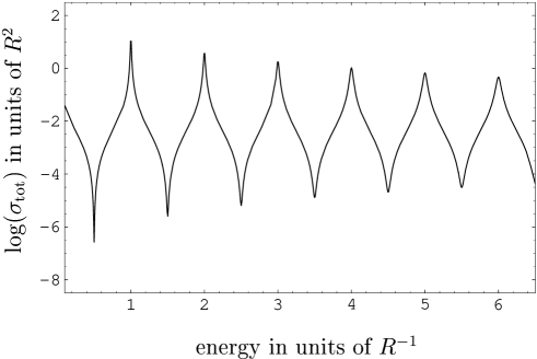
Figure 2: Total cross section for $e^{+}e^{-}\to\mu^{+}\mu^{-}$ as a function of center-of-mass energy on a logarithmic scale. The width of the KK modes has been reasonably approximated

The VEV introduces an additional mass term for each KK mode of the gauge fields. The zero mode turns from a massless to a massive degree of freedom, as usual for the Higgs mechanism. All the higher KK masses are slightly shifted. The gauge and self interactions of the Higgs fields, omitted in (24), only involve bulk fields, in contrast to the photon-fermion interaction introduced before. Although this leads to interesting effects we postpone their discussion until Sect. 3 where we investigate the phenomenologically more interesting gauge-boson self-couplings. After spontaneous symmetry breaking, it is instructive to introduce the fields

$$G_{(n)}\,=\,\Big{(}\,\frac{n^{2}}{R^{2}}\>+\>e^{2}v^{2}\,\Big{)}^{-1/2}\,\left(\,\frac{n}{R}\,A_{(n)5}\>+\>ev\,\chi_{(n)}\,\right)\,,$$ (26)

where again $e=e_{5}/\sqrt{2\pi R}$, and the orthogonal linear combinations $a_{(n)}$. In the effective kinetic Lagrangian of the theory for the $n$-KK mode ($n>0$)

$$\begin{split}\mathcal{L}^{(n)}_{\mathrm{kin}}(x)\,=&\,-\,\frac{1}{4}\,F_{(n)}^{\mu\nu}\,F_{(n)\mu\nu}\\ &\,\,+\,\frac{1}{2}\,\left(m_{A(n)}\,A_{(n)\mu}\,+\,\partial_{\mu}\,G_{(n)}\right)\,\left(m_{A(n)}\,A^{\mu}_{(n)}\,+\,\partial^{\mu}\,G_{(n)}\right)\\[4.30554pt] &\,\,+\,\frac{1}{2}\,(\partial_{\mu}a_{(n)})\,(\partial^{\mu}a_{(n)})\>-\>\frac{1}{2}m^{2}_{a(n)}a_{(n)}^{2}\ +\ \dots\,,\end{split}$$ (27)

$G_{(n)}$ now plays the rôle of a Goldstone mode in an Abelian Higgs model. Both, $A_{(n)5}$ and $\chi_{(n)}$ take part in the mass generation for the heavy KK modes and, therefore, they are also mixed in the corresponding Goldstone mode. Because the mass contribution from spontaneous symmetry breaking is expected to be small compared to the KK masses, the Goldstone modes are dominated by the extra component of the gauge field. The pseudoscalar field $a_{(n)}$ describes an additional physical KK excitation degenerate in mass with the KK gauge mode $A_{(n)\mu}$, i.e.

$$m^{2}_{a(n)}=m^{2}_{A(n)}=(n^{2}/R^{2})+e^{2}v^{2}\,.$$ (28)

The spectrum of the zero KK modes is simply identical to that of a conventional Abelian Higgs model, as it should be if we are to rediscover known physics in the low energy limit. It becomes clear that the appropriate gauge-fixing Lagrangian in (21) for a 5-dimensional generalized $R_{\xi}$-gauge should be

$${\mathcal{L}}_{\mathrm{GF}}(x,y)\,=\,-\,\frac{1}{2\xi}\,\bigg{[}\,\partial_{\mu}A^{\mu}\,-\,\xi\,\bigg{(}\,\partial_{5}A_{5}\>+\>e_{5}\frac{v}{\sqrt{2\pi R}}\,\chi\,\bigg{)}\,\bigg{]}^{2}\,.$$ (29)

All the mixing terms are removed and we again arrive at the standard kinetic Lagrangian for massive gauge bosons and the corresponding would-be Goldstone modes

$$\begin{split}\mathcal{L}^{(n)}_{\mathrm{kin}}(x)\ =\ &-\frac{1}{4}\,F_{(n)}^{\mu\nu}\,F_{(n)\mu\nu}\>+\>\frac{1}{2}\,m_{A(n)}^{2}\,A_{(n)\mu}\,A^{\mu}_{(n)}\>-\>\frac{1}{2\xi}(\partial_{\mu}\,A_{(n)}^{\mu})^{2}\\[4.30554pt] &+\,\frac{1}{2}(\partial_{\mu}G_{(n)})\,(\partial^{\mu}G_{(n)})\>-\>\frac{\xi}{2}\,m_{A(n)}^{2}\,G_{(n)}^{2}\\[4.30554pt] &+\,\frac{1}{2}(\partial_{\mu}a_{(n)})\,(\partial^{\mu}a_{(n)})\>-\>\frac{1}{2}\,m_{a(n)}^{2}\,a_{(n)}^{2}\\[4.30554pt] &+\,\frac{1}{2}(\partial_{\mu}h_{(n)})\,(\partial^{\mu}h_{(n)})\>-\>\frac{1}{2}\,m_{h(n)}^{2}\,h_{(n)}^{2}\,\,\,.\end{split}$$ (30)

The CP-odd scalar modes $a_{(n)}$ and the Higgs KK-modes $h_{(n)}$ with mass

$$m_{h(n)}=\sqrt{(n^{2}/R^{2})+\lambda_{5}v^{2}/\pi R}$$ (31)

are not affected by the gauge fixing procedure. Observe finally that the limit $\xi\to\infty$ consistently corresponds to the unitary gauge.

As a qualitatively different way of implementing the Higgs sector in a higher-dimensional Abelian model, we can localize the Higgs field at the $y=0$ boundary of the $S^{1}/Z_{2}$ orbifold, following the example of the fermions in 5D-QED. Introducing the appropriate $\delta$-function in the 5-dimensional Lagrangian, this amounts to

$${\mathcal{L}}(x,y)\ =\ -\,\frac{1}{4}\,F^{MN}\,F_{MN}\>+\>\delta(y)\,\left[\,(D_{\mu}\Phi)^{*}\,(D^{\mu}\Phi)\>-\>V(\Phi)\,\right]\>+\>{\mathcal{L}}_{\mathrm{GF}}(x,y)\,,$$ (32)

where the covariant derivative is given by (18) and the Higgs potential has its familiar 4-dimensional form. Because the Higgs potential is effectively four dimensional the Higgs field, not having KK excitations as a brane field, acquires the usual VEV. Notice that the bulk scalar field $A_{5}(x,y)$, as a result of its odd $Z_{2}$-parity, does not couple to the Higgs sector on a brane.

After compactification and integration over the $y$-dimension, spontaneous symmetry breaking again generates masses for all the KK gauge modes $A^{\mu}_{(n)}$. However, the mass matrix for the simple Fourier modes in (9) is no longer diagonal because of the $\delta$-function in (32). Instead, it is given by

$$M_{A}^{2}\,=\,\left(\begin{array}[]{cccc}m^{2}&\sqrt{2}\,m^{2}&\sqrt{2}\,m^{2}&\cdots\\ \sqrt{2}\,m^{2}&2\,m^{2}+(1/R)^{2}&2\,m^{2}&\cdots\\ \sqrt{2}\,m^{2}&2\,m^{2}&2\,m^{2}+(2/R)^{2}&\cdots\\ \vdots&\vdots&\vdots&\ddots\end{array}\right)\quad,$$ (33)

where $m=ev$. Therefore, the Fourier modes are no longer mass eigenstates. By diagonalization of the mass matrix the mass eigenvalues $m_{(n)}$ of the KK mass eigenstates are found to obey the transcendental equation

$$m_{(n)}\,=\,\pi\,m^{2}\,R\,\cot\left(\,\pi\,m_{(n)}\,R\,\right)\,.$$ (34)

Hence, the zero-mode mass eigenvalues are slightly shifted from what we expect in a 4D model. An approximate calculation, to first order in $m^{2}/M^{2}$, yields

$$m_{(0)}\,\approx\,\left(\,1-\frac{\pi^{2}}{6}\,\frac{m^{2}}{M^{2}}\,\right)\,\,m\,.$$ (35)

The respective KK mass eigenstates can also be calculated analytically. They are given by

$$\hat{A}^{\mu}_{(n)}\!=\!\left(1+\pi^{2}\,m^{2}\,R^{2}+\frac{m^{2}_{(n)}}{m^{2}}\right)^{\!\!\!-1/2}\sum^{\infty}_{j=0}\,\frac{2\,m_{(n)}\,m}{m^{2}_{(n)}\,-\,(j/R)^{2}}\,\left(\frac{1}{\sqrt{2}}\right)^{\delta_{j,0}}\,A^{\mu}_{(j)}\,.$$ (36)

The couplings of these mass eigenstates to fermions will be slightly shifted with respect to the couplings of the Fourier modes in (20). To be specific, the interaction Lagrangian can be parameterized by

$$\mathcal{L}_{\mathrm{int}}\,=\,-\,\overline{\Psi}\,\gamma_{\mu}\Psi\,\sum_{n=0}^{\infty}\,e_{(n)}\,\hat{A}^{\mu}_{(n)}\,,$$ (37)

where the couplings $e_{(n)}$ of the different mass eigenstates are given by

$$e_{(n)}\,=\,\sqrt{2}\,e\,\left(\,1\,+\,\frac{m^{2}}{m^{2}_{(n)}}\,+\,\pi^{2}\,\frac{m^{2}}{M^{2}}\frac{m^{2}}{m^{2}_{(n)}}\,\right)^{-\frac{1}{2}}\quad.$$ (38)

For example, the shift in the zero mode coupling is approximately given by

$$e_{(0)}\,\approx\,\left(\,1\,-\,\frac{\pi^{2}}{3}\,\frac{m^{2}}{M^{2}}\,\right)e\,.$$ (39)

Here, in the Abelian model, the shifts in masses and couplings may seem to be a mere matter of redefinition of the measured masses and coupling in terms of the fundamental constants of the 5D-theory. However, they lead to important phenomenological implications in the context of the higher-dimensional Standard Model, where the various couplings are affected differently, as we will see below.

To find the appropriate form of the gauge-fixing term ${\mathcal{L}}_{\mathrm{GF}}(x,y)$ in (32), we follow (29), but restrict the scalar field $\chi$ to the brane $y=0$, viz.

$${\mathcal{L}}_{\mathrm{GF}}(x,y)\,=\,-\,\frac{1}{2\xi}\,\Big{[}\,\partial_{\mu}A^{\mu}\ -\ \xi\,\big{(}\partial_{5}\,A_{5}\>+\>e_{5}v\,\chi\,\delta(y)\big{)}\,\Big{]}^{2}\,.$$ (40)

As is expected from a generalized $R_{\xi}$ gauge, all mixing terms of the gauge modes $A_{(n)}^{\mu}$ with $A_{(n)5}$ and $\chi$ disappear up to total derivatives if $\delta(0)$ is appropriately interpreted on $S^{1}/Z_{2}$. Determining the unphysical mass spectrum of the Goldstone modes, we find a one-to-one correspondence of each physical vector mode of mass $m_{(n)}$ to an unphysical Goldstone mode with gauge-dependent mass $\sqrt{\xi}\,m_{(n)}$. In the unitary gauge $\xi\to\infty$, the would-be Goldstone modes are absent from the theory. The present brane-Higgs model does not predict other KK massive scalars apart from the physical Higgs boson $h$.

At this point, we cannot decide by any means which of the two possibilities for the Higgs sector, brane or bulk Higgs fields, could be realized in nature. Thus, we have to be ready to analyze both of them phenomenologically when we move on to SM extensions.

3 5-Dimensional Extensions of the Standard Model

It is a straightforward exercise to generalize the ideas introduced in Sect. 2 for non-Abelian theories

$$\begin{split}\mathcal{L}(x,y)\,=\,&-\,\frac{1}{4}\,F^{a}_{MN}F^{aMN}+\delta(y)\,\overline{\Psi}(x)\,\left(\,i\gamma^{\mu}\,D_{\mu}\,-\,m_{f}\right)\,\Psi(x)\\[4.30554pt] &\quad\quad+\,\mathcal{L}_{\mathrm{H}}\,+\,\mathcal{L}_{\mathrm{GF}}\,+\,\mathcal{L}_{\mathrm{FP}}\,,\end{split}$$ (41)

where the field strength for the non-Abelian gauge field of a group with structure constants $f^{abc}$ and coupling constant $g_{5}$ is given by

$$F^{a}_{MN}\,=\,\partial_{M}A^{a}_{N}\,-\,\partial_{N}A^{a}_{M}\,+\,g_{5}f^{abc}A^{b}_{M}A^{c}_{N}\,.$$ (42)

Compactification, spontaneous symmetry breaking and gauge fixing MPR ; DCH are very analogous to the Abelian case and the non-decoupling ghost sector can be easily included MPR . Hence, in the effective 4D theory, we arrive at a particle spectrum being similar to the Abelian case.

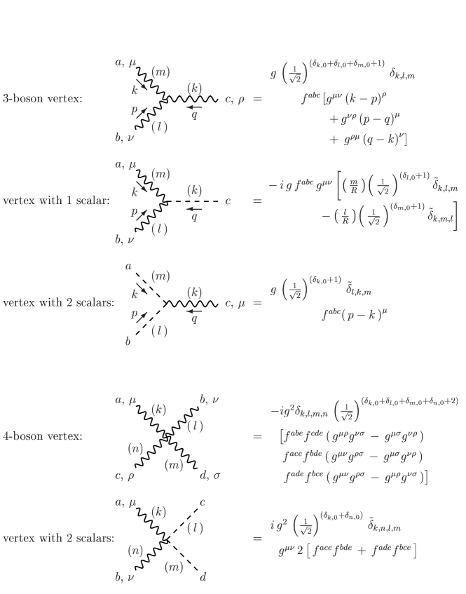
Figure 3: Feynman rules for the triple and quartic gauge boson couplings. The scalar modes correspond to the extra component of the higher-dimensional gauge fields. As in the Abelian model, they are would-be Goldstone modes and can be gauged away in unitary gauge. In parenthesis, the KK number of the interacting modes is shown. The selection rules are enforced by the prefactors defined in (43)

In addition, the self-interactions of the gauge bosons, induced by the bilinear terms in the non-Abelian field strength (42), lead to self-interactions of the KK modes which are restricted by selection rules, i.e., there are certain conditions for the KK numbers to be obeyed at each triple and quartic gauge-boson vertex. This is a general feature for interactions in which only bulk modes take part. A brane completely breaks the translational invariance of the orbifold and, thus, a brane field can couple to any bulk mode. In contrast, interactions between bulk fields obey a kind of quasi-momentum conservation with respect to the extra dimension, reflecting the special structure of the $S^{1}/Z_{2}$ orbifold and leading to the selection rules. The corresponding Feynman rules are displayed in Fig. 3. The selection rules are enforced by the prefactors

$$\begin{split}\delta_{k,l,m}&=\delta_{k+l+m,0}+\delta_{k+l-m,0}+\delta_{k-l+m,0}+\delta_{k-l-m,0}\,,\\ \tilde{\delta}_{k,l,m}&=-\delta_{k+l+m,0}+\delta_{k+l-m,0}-\delta_{k-l+m,0}+\delta_{k-l-m,0}\,,\end{split}$$ (43)

where $\delta_{i,j}$ denotes a standard Kronecker symbol. $\delta_{k,l,m,n}$ and $\tilde{\delta}_{k,l,m,n}$ are defined analogously.

At this point, we have considered all the important generic aspects of higher-dimensional theories. Therefore, we can now turn our attention to the theory we are really interested in, the electroweak sector of the Standard Model. Its gauge structure SU(2)${}_{L}\otimes$U(1)_Y opens up several possibilities for 5-dimensional extensions, because the SU(2)_L and U(1)_Y gauge fields do not necessarily both propagate in the extra dimension. As the fermion or Higgs fields we encountered before, one of the gauge groups can be confined to a brane at $y=0$. Such a realization of a higher-dimensional model may be encountered within specific stringy frameworks AB ; AKT .

However, in the most frequently investigated scenario, SU(2)_L and U(1)_Y gauge fields live in the bulk of the extra dimension (bulk-bulk model). The Lagrangian is simply an application of (41) to the Standard Model gauge groups. Here, it is possible, even before integrating out the extra dimension, to choose a basis for the fields, where the photon and $Z$-boson fields become explicit. The photon sector resembles exactly the 5D-QED discussed in Sect. 2, while for the $Z$ boson and its KK modes spontaneous symmetry breaking leads to the effects also presented in Sect. 2. In the bulk-bulk model, both a localized (brane) and a 5-dimensional (bulk) Higgs doublet can be included in the theory. For generality, we will consider a 2-doublet Higgs model, where the one Higgs field $\Phi_{1}$ propagates in the fifth dimension, while the other one $\Phi_{2}$ is localized. The phenomenology presented in these notes is not sensitive to details of the Higgs potential but only to their vacuum expectation values $v_{1}$ and $v_{2}$, or equivalently to $\tan\beta=v_{2}/v_{1}$ and $v^{2}=v^{2}_{1}+v^{2}_{2}$. Hence, $\beta$ is the only additional free parameter introduced in the model.

The chiral structure of the Standard Model can be easily incorporated as long as one only considers fermions restricted to a brane. A simple extension of (20) leads to

$${\mathcal{L}}_{\mathrm{int}}(x)\ =\ g\,\overline{\Psi}\,\gamma^{\mu}\,\left(\,g_{V}+g_{A}\gamma^{5}\,\right)\,\Psi\,\Big{(}A_{(0)\mu}\,+\,\sqrt{2}\,\sum_{n=1}^{\infty}A_{(n)\mu}\Big{)}\,,$$ (44)

where $A_{\mu}$ generically denotes some gauge boson and g the respective coupling constant. The coupling parameters $g_{V}$ and $g_{A}$ are set by the electroweak quantum numbers of the fermions and receive their SM values. Because the KK mass eigenmodes $\hat{A}_{(n)}^{\mu}$ generally differ from the Fourier modes $A_{(n)}^{\mu}$ in (44), as we have seen before, their couplings to fermions $g_{V(n)}$ and $g_{A(n)}$ have to be individually calculated for each model. The photon and its possible KK modes are not affected by spontaneous symmetry breaking and keep their simple couplings, already presented in Fig. 1. For the bulk-bulk model, the shifts in the vector and axial-vector couplings of the $Z$ boson are actually the same, such that it is sufficient to replace the SU(2) coupling constant $g$ by $g_{Z(n)}$ for each KK mode, in analogy to the Abelian Higgs model. The mass generation in the Yukawa sector, involving brane fermions, hardly changes at all.

An even more minimal 5-dimensional extension of electroweak physics constitutes a model in which only the U(1)_Y -sector feels the extra dimension while the SU(2)_L gauge fields are localized at $y=0$ (brane-bulk model). It is described by the Lagrangian

$$\begin{split}\mathcal{L}(x,y)=-\frac{1}{4}&B_{MN}\,B^{MN}\!+\delta(y)\!\left[-\frac{1}{4}\,F^{a}_{\mu\nu}F^{a\mu\nu}\!+\!\left(D_{\mu}\Phi\right)^{\dagger}\!\left(D^{\mu}\Phi\right)-V(\Phi)\right]\\[4.30554pt] &+\,\mathcal{L}_{\mathrm{GF}}(x,y)\ +\ \mathcal{L}_{\mathrm{FP}}(x,y)\,,\end{split}$$ (45)

where $\Phi$ denotes the Standard Model Higgs doublet on the brane and the covariant derivative

$$D_{\mu}\,=\,\partial_{\mu}\,-\,i\,g\,A^{a}_{\mu}(x)\,\tau^{a}\,-i\,\frac{g_{5}^{\prime}}{2}\,B_{\mu}(x,y)$$ (46)

involves a brane as well as a bulk field. The $W$ bosons are brane fields and their physics is completely SM-like. In this case, the Higgs field being charged with respect to both gauge groups has to be localized at $y=0$ in order to preserve gauge invariance of the (classical) Lagrangian. A gauge field on the brane cannot compensate the variation of a Higgs field under gauge transformations in the whole bulk. For the same reason, a bulk Higgs is forbidden in the third possible model in which U(1)_Y is localized while SU(2)_L propagates in the fifth dimension (bulk-brane model), i.e., the gauge groups interchange their rôle. Consequently, the $W$ bosons are bulk fields and are described in analogy to the models discussed in Sect. 2. In both models, after spontaneous symmetry breaking, there is a single massless gauge field protected by the residual unbroken gauge symmetry, the photon. A second light neutral mode can be identified with the $Z$ boson. However, in contrast to the bulk-bulk model, there is only a single neutral tower of heavy KK modes. Up to small admixtures due to the brane VEV (see Sect. 2), it mainly contains the U(1)_Y or the neutral SU(2)_L gauge field, respectively. Nevertheless, for simplicity, we will refer to it as $Z$-boson KK tower. Note, however, that $g_{V(n)}$ and $g_{A(n)}$ in (44) are affected differently for the $Z$-boson and its KK modes. Most easily they are parameterized by introducing effective quantum numbers $T_{3(n)}$ and $Q_{(n)}$ to absorb all the higher-dimensional effects.

After the setup of all the models, we can finally turn our attention to the actual predictions of higher-dimensional theories for experiment.

4 Effects on Electroweak Observables

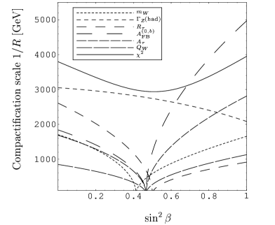
Figure 4: Lower bounds on $M=1/R$ (in TeV) from different observables at the 3$\sigma$ confidence level for the bulk-bulk model

In this section, we will concentrate on the phenomenology and present bounds on the compactification scale $M=1/R$ of minimal higher-dimensional extensions of the SM, calculated by analyzing a large number of observables. To be specific, we proceed as follows. We relate the SM prediction $\mathcal{O}^{\mathrm{SM}}$ PDG ; EWWG for an observable to the prediction $\mathcal{O}^{\mathrm{HDSM}}$ for the same observable obtained in the higher-dimensional SM under investigation through

$${\cal O}^{\rm HDSM}\ =\ {\cal O}^{\rm SM}\,\big{(}1\>+\>\Delta^{\rm HDSM}_{\cal O}\big{)}\,.$$ (47)

Here, $\Delta^{\rm HDSM}_{\cal O}$ is the tree-level modification of a given observable ${\cal O}$ from its SM value due to the presence of one extra dimension. The tree-level modifications can be expanded in powers of the typical scale factor

$$X\,=\,\frac{\pi^{2}}{3}\frac{m^{2}_{Z}}{M^{2}}\,\,.$$ (48)

We work to first order in $X$ being a very good approximation for phenomenologically viable compactification scales in the TeV region. On the other hand, to enable a direct comparison of our predictions with precise data PDG ; EWWG , we include SM radiative corrections to $\mathcal{O}^{\mathrm{SM}}$. However, we neglect SM- as well as KK-loop contributions to $\Delta^{\rm HDSM}_{\cal O}$ as higher order effects.

As input SM parameters for our numerical predictions, we choose the most accurately measured ones, namely the $Z$-boson mass $m_{Z}$, the electromagnetic fine structure constant $\alpha$, and the Fermi constant $G_{F}$. While $\alpha$ is not affected in the models under study, $m_{Z}=m_{Z(0)}$, the mass of the lightest mode in the $Z$ boson KK tower, generally deviates from its SM form, where we have $m_{Z}^{\mathrm{SM}}=\sqrt{g^{2}+g^{\prime}{}^{2}}\,v/2$ at tree level. To first order in $X$, $m_{Z}$ may be parameterized by

$$m_{Z}\ =\ m^{\mathrm{SM}}_{Z}\,\left(\,1\>+\>\Delta_{Z}\,X\,\right)\,,$$ (49)

where $\Delta_{Z}$ is a model-dependent parameter. For the bulk-bulk, brane-bulk and bulk-brane models with respect to the SU(2)_L and U(1)_Y gauge groups, $\Delta_{Z}$ is given by

$$\Delta_{Z}=\left\{\ -\,\frac{1}{2}\,\sin^{4}\beta\,,\ -\,\frac{1}{2}\,\sin^{2}\hat{\theta}_{W}\,,\ -\,\frac{1}{2}\,\cos^{2}\hat{\theta}_{W}\,\right\}\,,$$ (50)

where $\hat{\theta}_{W}$ is an effective weak mixing angle to be introduced below in (52). These shifts in the $Z$-boson mass are induced by the VEV of a brane Higgs.

Table 1: Lower bounds on $M=1/R$ (in TeV) at the 3$\sigma$ confidence level for the brane-bulk and bulk-brane models

Observable	U(1)Y in bulk		SU(2)L in bulk
$m_{W}$	1.2		1.2
$\Gamma_{Z}(\mathrm{had})$	0.8		2.3
$Q_{W}(\mathrm{Cs})$	0.4		0.8
$A_{\mathrm{FB}}^{(0,b)}$	4.4		2.4
$A_{\tau}$	2.5		1.4
$R_{\tau}$	1.0		0.5
global analysis	3.5		2.6

The Fermi constant $G_{F}$, as determined by the muon lifetime, may receive additional direct contributions due to KK states mediating the muon decay. We may account for this modification of $G_{F}$ by writing

$$G_{F}\ =\ G^{\mathrm{SM}}_{F}\,\left(\,1\>+\>\Delta_{G}\,X\,\right)\,,$$ (51)

where $\Delta_{G}$ is again model-dependent and has to be calculated consistently to first order in $X$.

The relation between the weak mixing angle $\theta_{W}$ and the input variables is also affected by the fifth dimension. Hence, it is useful to define an effective mixing angle $\hat{\theta}_{W}$ by

$$\sin^{2}\hat{\theta}_{W}\ =\ \sin^{2}\theta_{W}\,\left(\,1\>+\>\Delta_{\theta}\,X\,\right)\,,$$ (52)

such that the effective angle still fulfills the tree-level relation

$$G_{F}\ =\ \frac{\pi\alpha}{\sqrt{2}\sin^{2}\hat{\theta}_{W}\,\cos^{2}\hat{\theta}_{W}\,m_{Z}^{2}}\ ,$$ (53)

of the Standard Model.

Table 2: Lower bounds (in TeV) on the compactification scale $M=1/R$ at 2$\sigma$, 3$\sigma$ and 5$\sigma$ confidence levels from combined precision observables

model	2$\sigma$	3$\sigma$	5$\sigma$
SU(2)L-brane, U(1)Y-bulk	4.3	3.5	2.7
SU(2)L-bulk, U(1)Y-brane	3.0	2.6	2.1
SU(2)L-bulk, U(1)Y-bulk (brane Higgs)	4.7	4.0	3.1
SU(2)L-bulk, U(1)Y-bulk (bulk Higgs)	4.6	3.8	3.0

For the tree-level calculation of $\Delta^{\rm HDSM}_{\cal O}$, we have to carefully consider the effects from mixing of the Fourier modes on the masses of the Standard-Model gauge bosons as well as on their couplings to fermions. In addition, we have to keep in mind that the mass spectrum of the KK gauge bosons also depends on the model under consideration.

Within the framework outlined above, we first compute $\Delta^{\rm HDSM}_{\cal O}$ for the following high precision observables to first order in $X$: the $W$-boson mass $m_{W}$, the $Z$-boson invisible width $\Gamma_{Z}(\nu\overline{\nu})$, $Z$-boson leptonic widths $\Gamma_{Z}(l^{+}l^{-})$, the $Z$-boson hadronic width $\Gamma_{Z}(\mathrm{had})$, the weak charge of cesium $Q_{W}$ measuring atomic parity violation, various ratios $R_{l}$ and $R_{q}$ involving partial $Z$-boson widths, fermionic asymmetries $A_{f}$ at the $Z$ pole, and various fermionic forward-backward asymmetries $A_{\mathrm{FB}}^{(0,f)}$. For example, for the invisible $Z$ width $\Gamma_{Z}(\nu\overline{\nu})$ we obtain

$$\Delta^{\rm HDSM}_{\Gamma_{Z}(\nu\overline{\nu})}=\left\{\begin{array}[]{cl}\sin^{2}\!\hat{\theta}_{W}\,\left(\,\!\sin^{2}\!\beta-1\!\,\right)^{2}-1&\mbox{for the bulk-bulk model,}\\[4.30554pt] -\sin^{2}\!\hat{\theta}_{W}&\mbox{for the brane-bulk model,}\\[4.30554pt] -\cos^{2}\!\hat{\theta}_{W}&\mbox{for the bulk-brane model.}\end{array}\right.$$ (54)

Employing the results for $\Delta^{\mathrm{HDSM}}_{\mathcal{O}}$ and calculating all the electroweak observables considered in our analysis by virtue of (47), we confront these predictions with the respective experimental results. We can either test each variable individually or perform a $\chi^{2}$ test to obtain combined bounds on the compactification scale $M=1/R$, where

$$\chi^{2}(R)\ =\ \sum_{i}\,\frac{\left(\,\mathcal{O}_{i}^{\mathrm{exp}}\>-\>\mathcal{O}_{i}^{\mathrm{HDSM}}\,\right)^{2}}{\left(\,\Delta\mathcal{O}_{i}\,\right)^{2}}\,,$$ (55)

$i$ runs over all the observables, and $\Delta\mathcal{O}_{i}$ is the combined experimental and theoretical error. A compactification radius is considered to be compatible at the $n\sigma$ confidence level (CL) if $\chi^{2}(R)-\chi^{2}_{\mathrm{min}}<n^{2}$, where $\chi^{2}_{\mathrm{min}}$ is the minimum of $\chi^{2}$ for a compactification radius in the physical region, i.e. for $R^{2}>0$.

Figure 4 summarizes the lower bounds on the compactification scale $M$ inferred from different types of observables for the bulk-bulk model. In this model, we present the bounds as a function of $\sin^{2}\beta$ parameterizing the Higgs sector. In Table 1, we summarize the bounds obtained by our calculations for the two bulk-brane models. The bounds from the global analysis at different confidence levels are shown in Table 2. The global $2\sigma$ bounds lie in the $4\sim 5$ TeV region, only the bulk-brane model is less restricted. Here, a compactification scale of 3 TeV cannot be excluded by electroweak precision observables.

Table 3: 2$\sigma$ bounds in TeV inferred from fermion-pair production

model	$\mu^{+}\mu^{-}$	$\tau^{+}\tau^{-}$	hadrons	$e^{+}e^{-}$
SU(2)L-brane, U(1)Y-bulk	2.0	2.0	2.6	3.0
SU(2)L-bulk, U(1)Y-brane	1.5	1.5	4.7	2.0
SU(2)L-bulk, U(1)Y-bulk (brane Higgs)	2.5	2.5	5.4	3.6
SU(2)L-bulk, U(1)Y-bulk (bulk Higgs)	2.5	2.5	5.8	3.5

While the precision observables, analyzed so far, are measured at the $Z$ pole or even at low energies, LEP2 provides us with data on cross sections at higher energies, up to more than 200 GeV. At these energies, the interference terms between Standard Model and KK contributions to a process like fermion-pair production dominate the higher-dimensional effects. In a first approximation, they are only suppressed by a factor of order $s/M^{2}$, where $\sqrt{s}$ is the center-of-mass energy, compared to the typical scale factor $X$ of mass mixings and coupling shifts. Higher energies naturally lead to more sensitivity with respect to a possible fifth dimension CL ; MPR2 ; MN . As the simplest example for LEP2 processes, let us have a closer look at fermion-pair production. The relevant differential cross section for these observables is given at tree level by

Table 4: 2$\sigma$ bounds in TeV inferred from precision observables and LEP2 cross sections

model	LEP1	LEP2	combined
SU(2)L-brane, U(1)Y-bulk	4.3	3.5	4.7
SU(2)L-bulk, U(1)Y-brane	3.0	4.4	4.3
SU(2)L-bulk, U(1)Y-bulk (brane Higgs)	4.7	5.4	6.1
SU(2)L-bulk, U(1)Y-bulk (bulk Higgs)	4.6	5.7	6.4

$$\begin{split}\frac{\sigma(e^{+}e^{-}\to f\,\overline{f})}{d\,\cos\theta}=\frac{s}{128\,\pi}&\left[(1+\cos\theta)^{2}\,(|M^{ef}_{LL}(s)|^{2}+|M^{ef}_{RR}(s)|^{2})\,\,+\right.\\ &\,\,\,\left.(1-\cos\theta)^{2}\,(|M^{ef}_{LR}(s)|^{2}+|M^{ef}_{RL}(s)|^{2})\right]\,,\end{split}$$ (56)

where $\theta$ is the scattering angle between the incoming electron and the negatively charged outgoing fermion, and

$$M^{ef}_{\alpha\beta}(s)=\sum_{n=0}^{\infty}\left(\,e_{(n)}^{2}\,\frac{Q_{e}Q_{f}}{s-m^{2}_{\gamma(n)}}\,+\,\frac{g^{e}_{\alpha(n)}g^{f}_{\beta(n)}}{\cos^{2}\theta_{W}}\,\frac{1}{s-m^{2}_{Z(n)}}\,\right)\,.$$ (57)

The couplings $g^{f}_{L(n)}$ and $g^{f}_{R(n)}$ in turn are given by

$$\begin{split}g^{f}_{L(n)}&=g_{Z(n)}\left(\,T_{3f(n)}-Q_{f(n)}\sin^{2}\theta_{W}\,\right)\,,\\ g^{f}_{R(n)}&=g_{Z(n)}\left(\,-Q_{f(n)}\sin^{2}\theta_{W}\,\right)\,.\end{split}$$ (58)

$T_{3f(n)}$, $Q_{f(n)}$, $g_{Z(n)}$, $e_{(n)}$, $m_{Z(n)}$ and $m_{\gamma(n)}$, as introduced in Sect. 3, can be calculated to first order in $X$, e.g. from the exact analytic expressions in MPR . For Bhabha scattering the $t$-channel exchange also has to be taken into account, however, there are no fundamental differences. The above parameterization for the cross section is particularly convenient because it clearly separates the higher-dimensional effects from well known physics. All the higher-dimensional physics manifests itself in the effective sum of s-channel propagators (57) differing with respect to the Standard Model.

From (56), we calculate $\Delta^{\rm HDSM}_{\cal O}$ for the different fermion-pair production channels at LEP2 energies and finally the bounds shown in Table 3. In Table 4, all the bounds are combined for final lower limits on the compactification scale. The bounds for the brane-bulk and the bulk-brane models from LEP1 and LEP2 observables are kind of complementary, such that the combined limit is larger than 4 TeV in both models. The compactification scale for the bulk-bulk model, no matter where the Higgs lives, is still more restricted to lie above 6 TeV at the $2\sigma$ confidence level.

5 Conclusions

The aim of the present notes has been to give an introduction to the model-building of low-energy 5-dimensional electroweak models. We have derived step by step the corresponding four dimensional theory by compactifying on the orbifold $S^{1}/Z_{2}$ and by integrating out the extra dimension. We have paid special attention to consistently quantize the higher-dimensional models in the generalized $R_{\xi}$ gauges. The 5-dimensional $R_{\xi}$ gauge fixing conditions introduced here lead, after compactification, to a 4-dimensional Lagrangian in the standard $R_{\xi}$ gauge for each KK mode. The latter also clarifies the rôle of the different degrees of freedom. One of the main advantages of our gauge-fixing procedure is that one can now derive manifest gauge-independent analytic expressions for the KK-mass spectrum of the gauge bosons and for their interactions to the fermionic matter. Most importantly, one may even apply an analogous gauge-fixing approach to spontaneous symmetry breaking theories.

To render the topics under discussion more intuitive, we have analyzed all the main ideas in simple Abelian toy models. However, we have pointed out how to generalize these ideas to new possible 5-dimensional extensions of the SM in which the SU(2)_L and U(1)_Y gauge fields and Higgs bosons may or may not all experience the presence of the fifth dimension. The fermions in all the models are considered to be confined to one of the two boundaries of the $S^{1}/Z_{2}$ orbifold.

After introducing a framework for deriving predictions of possible observables, we have given a glimpse of higher-dimensional phenomenology. Electroweak precision observables are considered as well as cross sections for fermion-pair production at LEP2. In particular, we have presented bounds on the compactification scale $M=1/R$ in three different 5-dimensional extensions of the SM: (i) the SU(2)${}_{L}\otimes$U(1)_Y-bulk model, where all SM gauge bosons are bulk fields; (ii) the SU(2)_L-brane, U(1)_Y-bulk model, where only the $W$ bosons are restricted to the brane, and (iii) the SU(2)_L-bulk, U(1)_Y-brane model, where only the U(1)_Y gauge field is confined to the brane. For the often-discussed first model, we find the 2$\sigma$ lower bounds on $M$: $M\stackrel{{\scriptstyle>}}{{{}_{\sim}}}6.4$ and 6.1 TeV, for a Higgs boson living in the bulk and on the brane, respectively. For the second and third models, the corresponding 2$\sigma$ lower limits are 4.7 and 4.3 TeV. Hence, the bounds for different models can differ significantly.

Any non-stringy field-theoretic treatment of higher-dimensional theories, as the one presented here, involves a number of assumptions. Although the results obtained in the higher-dimensional models with one compact dimension are convergent at the tree level, they become divergent if more than one extra dimensions are considered. Also, the analytic results are ultra-violet (UV) divergent at the quantum level, since the higher-dimensional theories are not renormalizable. Within a string-theoretic framework, the above UV divergences are expected to be regularized by the string mass scale $M_{s}$. Therefore, from an effective field-theory point of view, the phenomenological predictions will depend to some extend on the UV cut-off procedure KMZ related to the string scale $M_{s}$. Nevertheless, assuming validity of perturbation theory, we expect that quantum corrections due to extra dimensions will not exceed the 10% level of the tree-level effects we have been studying here. Finally, we have ignored possible model-dependent winding-number contributions ABL and radiative brane effects Georgi that might also affect to some degree our phenomenological predictions.

The lower limits on the compactification scale derived by the present global analysis indicate that resonant production of the first KK state may be at the edge of accessibility at the LHC, at which heavy KK masses up to 6–7 TeV AB ; RW might be explored. Hence, the phenomenological analysis has to be carried further in order to be able to discriminate possible higher-dimensional signals from other Standard Model extensions.

Acknowledgements

This work was supported by the Bundesministerium für Bildung and Forschung (BMBF, Bonn, Germany) under the contract number 05HT1WWA2.

References

- (1) T. Kaluza: Sitzungsber. d. Preuss. Akad. d. Wiss. Berlin, 966 (1921) O. Klein: Zeitschrift f. Physik 37 895 (1926)
- (2) For a review, see e.g., M.B. Green, J.H. Schwarz, E. Witten: Superstring Theory. (Cambridge University Press, Cambridge 1987).
- (3) I. Antoniadis: Phys. Lett. B 246, 377 (1990)
- (4) J.D. Lykken: Phys. Rev. D 54 3693 (1996)
- (5) E. Witten: Nucl. Phys. B 471 135 (1996) P. Hoava, E. Witten: Nucl. Phys. B 460 506 (1996); Nucl. Phys. B 475 94 (1996)
- (6) N. Arkani-Hamed, S. Dimopoulos, G. Dvali: Phys. Lett. B 429 263 (1998) I. Antoniadis, N. Arkani-Hamed, S. Dimopoulos, G. Dvali: Phys. Lett. B 436 257 (1998); N. Arkani-Hamed, S. Dimopoulos, G. Dvali: Phys. Rev. D 59 086004 (1999)
- (7) K.R. Dienes, E. Dudas, T. Gherghetta: Phys. Lett. B 436 55 (1998); Nucl. Phys. B 537 47 (1999)
- (8) I. Antoniadis, K. Benakli: Int. J. Mod. Phys. A 15 4237 (2000)
- (9) I. Antoniadis, E. Kiritsis, T.N. Tomaras: Phys. Lett. B 486 186 (2000)
- (10) P. Nath, M. Yamaguchi: Phys. Rev. D 60 116006 (1999); Phys. Lett. B 466 100 (1999)
- (11) W.J. Marciano: Phys. Rev. D 60 093006 (1999); M. Masip, A. Pomarol: Phys. Rev. D 60 096005 (1999)
- (12) R. Casalbuoni, S. De Curtis, D. Dominici, R. Gatto: Phys. Lett. B 462 48 (1999); C. Carone: Phys. Rev. D 61 015008 (2000)
- (13) A. Delgado, A. Pomarol, M. Quiros: JHEP 0001 030 (2000)
- (14) T. Rizzo, J. Wells: Phys. Rev. D 61 016007 (2000); A. Strumia: Phys. Lett. B 466 107 (1999)
- (15) A. Delgado, A. Pomarol, M. Quiros: Phys. Rev. D 60 095008 (1999)
- (16) K. Cheung, G. Landsberg: Phys. Rev. D 65 076003 (2002)
- (17) A. Mück, A. Pilaftsis, R. Rückl: Phys. Rev. D 65 085037 (2002)
- (18) For example, see H. Georgi, A.K. Grant, G. Hailu: Phys. Lett. B 506 207 (2001)
- (19) D.M. Ghilencea, S. Groot Nibbelink, H.P. Nilles: Nucl. Phys. B 619 385 (2001)
- (20) J. Papavassiliou, A. Santamaria: Phys. Rev. D 63 125014 (2001)
- (21) D. Dicus, C. McMullen, S. Nandi: Phys. Rev. D 65 076007 (2002)
- (22) T. Appelquist, H.C. Cheng and B.A. Dobrescu: Phys. Rev. D 64 035002 (2001)
- (23) R.S. Chivukula, D.A. Dicus, H.-J. He: Phys. Lett. B 525 175 (2002)
- (24) Particle Data Group (D.E. Groom et al.): European Physical Journal C 15 1 (2000)
- (25) The LEP Collaborations ALEPH, DELPHI, L3, OPAL, the LEP Electroweak Working Group and the SLD Heavy Flavor and Electroweak Groups: hep-ex/0112021
- (26) A. Mück, A. Pilaftsis, R. Rückl: work in preparation
- (27) C.D. McMullen, S. Nandi: hep-ph/0110275
- (28) T. Kobayashi, J. Kubo, M. Mondragon and G. Zoupanos, Nucl. Phys. B 550 99 (1999)
- (29) I. Antoniadis, K. Benakli and A. Laugier, JHEP 0105 044 (2001)
- (30) H. Georgi, A.K. Grant, G. Hailu, Phys. Lett. B 506 207 (2001) M. Carena, T. Tait, C.E.M. Wagner: hep-ph/0207056