Beyond-Constant-Mass-Approximation Magnetic Catalysis in the Gauge Higgs-Yukawa Model

Abstract

Beyond-constant-mass approximation solutions for magnetically catalyzed fermion and scalar masses are found in a gauge Higgs-Yukawa theory in the presence of a constant magnetic field. The obtained fermion masses are several orders of magnitude larger than those found in the absence of Yukawa interactions. The masses obtained within the beyond-constant-mass approximation exactly reduce to the results within the constant-mass approach when the condition $\nu\ln(\frac{1}{\widehat{m}^{2}})\ll 1$ is satisfied. Possible applications to early universe physics and condensed matter are discussed. PACS numbers: 11.30Qc; 11.30 Rd; 12.15-y; 12.20.Ds

I Introduction

In the last few years the magnetic catalysis (MC) of chiral symmetry breaking [1]-[3] has been the focus of attention of many works on non-perturbative effects of magnetic fields [1]-[21]. The phenomenon consists on the dynamical generation of a fermion condensate (and consequently of a fermion mass) when the fermion interactions occur in the presence of an external constant magnetic field. A most significant feature of the MC is that it requires no critical value of the fermion’s coupling for the condensate to be generated. That is, the symmetry breaking takes place at the weakest attractive interaction. Physically it is due to the fact that the magnetic field forces the low energy fermions to reside basically in their lowest Landau level (LLL), while the higher energy fermions actually decouple [8]. This, in turn, yields a dimensional reduction of the infrared fermion dynamics. The dimensional reduction is reflected in an effective strengthening of the fermion interactions leading to dynamical symmetry breaking through the generation of a fermion condensate.

A particularly important question to understand in this context is how the MC is affected by the introduction of fermion-scalar interactions. Fermion-scalar interactions are an essential element of the unified theories of fundamental forces. As is well known, they are expected to be responsible for the fermion mass appearing due to the spontaneous symmetry breaking of the electroweak symmetry. Fermion-scalar interactions are also relevant in condensed matter physics where the complexity of strongly-correlated many-body systems some times calls for a description in terms of more simple, phenomenological theories that contain interacting scalar in addition to fermions (see e.g. [22]).

In Refs. [12]-[13] two of us studied the realization of magnetic catalysis in a (3+1)-dimensional Higgs-Yukawa (HY) model, showing that the magnetic-field-induced fermion mass is enhanced by fermion-scalar interactions. As we will show below, this enhancement is also found within a more accurate approximation for a wide range of couplings. This result might find applications in early universe transitions, as well as in condensed matter physics.

In [12]-[14] some applications of the MC to the early universe were briefly considered. They were motivated by many astrophysical observations of galactic and intergalactic magnetic fields indicating the existence of seed fields that originated from large primordial magnetic fields (for a recent review on cosmic magnetic fields see [23]). If the primordial magnetic fields in the early universe were large compared to the values close to the phase transition point of the fermion masses generated through the usual mechanism of spontaneous symmetry breaking, the fermion would seem approximately massless. Under these circumstances, it is important to investigate if the primordial magnetic fields could contribute to the masses of the fermions through MC and hence influence the phenomenology of the early universe [13].

On the other hand, to discuss applications of MC in the context of a HY theory to condensed matter, we need, besides interactions modelled by fermion-scalar terms, a physical system that, despite being non-relativistic, can be described under certain conditions by a ”relativistic” Hamiltonian. We will see below that these conditions are indeed present in the physics of high-$T_{c}$ superconductors.

High-$T_{c}$ superconductors, which are characterized by the existence of nodal points where the order parameter (gap function) vanishes, provide a practical realization of a ”relativistic” system in condensed matter physics. This is so because the low-energy spectrum of the nodal quasiparticles is linear, hence the quasiparticle excitations are described by an anisotropic Dirac Hamiltonian [24]. In Ref. [22] a quantum-critical phase transition to a new superconducting state, characterized by the appearance of a secondary pairing at some doping level, was proposed to explain recent measurements [25] of an anomalously large inelastic scattering of quasiparticles near the gap nodes of a superconductor. The observed secondary pairing transition made the nodal quasiparticles fully gapped. Based on the symmetries of the superconductor, the authors of Ref. [22] made a classification of a set of fermion-scalar interactions that in principle could be in agreement with the experimental observations, and then performed a perturbative renormalization-group analysis of each model to determine the possible existence of a quantum-critical point. In Ref. [26], expanding on the ideas of [22], the existence of a quantum critical point was established directly in a (2+1)-dimensional HY theory beyond a non-perturbative approach, which allowed to make quantitative predictions for the corresponding quantum-critical behavior. The gap generation (fermion mass) was associated in [26] with the breaking of a discrete chiral symmetry.

We would like to underline that the breaking of the chiral symmetry in [26] was found to occur when the Yukawa coupling (assumed to be related to the doping level) reached a critical value, that is, the symmetry breaking was not associated to the phenomenon of MC, as no external magnetic field was introduced in the analysis. However, as recently observed [27] by measuring the splitting of the conductance peak that characterizes the nodes of high-$T_{c}$ superconductors, the development of a secondary quasiparticle gap may be triggered not only by the doping level, but also by an applied magnetic field. Could the secondary gap triggered by the magnetic field be the consequence of MC occurring within the superconductor? We believe that the results we are going to derive below strongly indicate that the answer is yes, if, as argued in [22] and [26], the HY theory is the model describing the appearing of the secondary gap. Nevertheless, to match the experimental observations we would need to particularize the analysis done in the present paper to the (2+1)-dimensional case, and adjust the physical values of the couplings to those characteristic of the superconductor.

As already mentioned, in Ref. [13] the phenomenon of MC in a (3+1)-dimensional Abelian gauge theory with HY interactions was studied. In that work it was shown that the non-perturbative solution of the minimum equations for the composite-operator effective action leads not only to a magnetically catalyzed fermion dynamical mass, but also to a nonzero scalar vev $\varphi_{c}$ and consequently, to a nonzero scalar mass. In other words, thanks to the magnetic field, a scalar-field minimum solution is generated by non-perturbative radiative corrections.

We should underline though that the fermion and scalar masses of ref. [13] were obtained within a simplified approximation known in the literature as the constant mass approximation (CMA). In general, to find the dynamical mass —which is nothing but the part of the fermion self-energy proportional to the identity matrix— one has to solve a non-perturbative gap equation (i.e. the Schwinger-Dyson equation for the full fermion propagator). This means to solve a non-linear, implicit integral equation for the fermion self-energy, which is a momentum-dependent function. Most authors approach such a mathematically complicated problem with the help of the rough CMA approach. It consists on neglecting the momentum dependence of the self-energy in the gap equation. This is done by substituting the self-energy function in the gap equation by its value at zero momentum, that is, by the infrared mass. There is no general principle that guarantees the validity of this approximation for the whole range of physical couplings.

For theories with several couplings, due to the richness of the parameter space, the reliability of the CMA is questionable and should be investigated in detail. In the case of the HY model, aside from the multiple-coupling problem, one has to deal with a system of non-linear, coupled integral equations, one for the fermion dynamical mass and other for the scalar vev [13]. We cannot disregard in this situation the possibility of regions of these parameters where the CMA is reliable and regions where it is not. In this case one has to turn to a more accurate approximation on which the momentum dependence of the self-energy is taken into account when solving the gap equation. This more accurate approximation is known as the beyond-constant-mass approximation (BCMA).

For theories like QED containing only one coupling constant, the CMA is known to be appropriate, since going beyond it does not produce qualitatively different results. This has been explicitly shown for (3+1)-dimensional [2] and (2+1)-dimensional QED [28], and independently corroborated by our calculations below. In Ref. [9] the BCMA mass solution of (3+1)-dimensional QED was found to agree with the CMA mass obtained from the improved-ladder gap equation. This result was later corroborated by numerical calculations in [29].

Considering that different physical applications of the MC in models with fermion-scalar interactions would require different values of the couplings constants, and in particular, given the relevance that the Abelian gauge Higgs-Yukawa theory may have for condensed matter and other field theory applications, it is important to perform a BCMA investigation of this model in all possible regions of the parameter space and find out whether it significantly differs or not from the CMA results. A main goal of the present paper is to carry out such a study.

By going beyond the CMA, we will determine the region of Yukawa and scalar self-interaction couplings where the CMA is valid, and will obtain the numerical BCMA solutions for the fermions and scalar dynamical masses in the complete physically meaningful parameter region. As we will see below, the CMA results for the Abelian gauge Higgs-Yukawa theory are mostly reliable in the available parameter space. An important finding is that the (BCMA-found) mass values are many orders of magnitude larger than those obtained in the absence of fermion-scalar interactions, corroborating, within this more accurate approximation, the enhancement of the dynamical mass by the Yukawa term.

The paper is organized as follows: In Section II we derive the non-linear integral equations for the fermion self energy (gap equation) and the scalar vev in a gauge Higgs-Yukawa theory. The integral gap equation is then converted into a second order differential equation with boundary conditions. In Section III, this boundary-value problem is analytically solved leading to the self energy as a function of the momentum and the infrared fermion mass. Using the self-energy solution and the equation for the scalar minimum, we arrive at two coupled transcendental equations depending on the infrared dynamical mass and the scalar vev. These equations are numerically solved and the results are used to determine the region of reliability of the CMA and to compare the mass values obtained in the CMA and in the BCMA approaches. We end Section III discussing the solution of the gap equation at zero Yukawa coupling, and showing that it leads to the same result found in Ref.[2] for (3+1)-dimensional QED. In Section IV, we state our concluding remarks and reconsider the question of the relevance of the magnetic catalysis in the electroweak phase transition using the BCMA results.

II Integral Equations

Let us consider the following Lagrangian density

$$L=-\frac{1}{4}F^{\mu\nu}F_{\mu\nu}+i\overline{\psi}\gamma^{\mu}\partial_{\mu}\psi+e\overline{\psi}\gamma^{\mu}\psi A_{\mu}-\frac{1}{2}\partial_{\mu}\varphi\partial^{\mu}\varphi-\frac{\lambda}{4!}\varphi^{4}-\frac{\mu^{2}}{2}\varphi^{2}-\lambda_{y}\varphi\overline{\psi}\psi$$ (1)

that describes a gauge Higgs-Yukawa model with a fermion field coupled to scalar and electromagnetic fields. The scalar field is electrically neutral, but self-interacting.

The Lagrangian density (1) has U(1) gauge symmetry,

$$A_{\mu} \rightarrow A_{\mu}+\frac{1}{e}\partial_{\mu}\alpha(x)$$ (2)

$$\psi \rightarrow e^{i\alpha(x)}\psi,$$ (3)

fermion number global symmetry

$$\psi\rightarrow e^{i\theta}\psi,$$ (4)

and discrete chiral symmetry

$$\psi\rightarrow\gamma_{{}_{5}}\psi,\qquad\overline{\psi}\rightarrow-\overline{\psi}\gamma_{{}_{5}},\qquad\varphi\rightarrow-\varphi.$$ (5)

Notice that the quadratic scalar term has the correct sign of a mass term, thus no vacuum expectation value of the scalar field exists at tree level. In the course of our calculations we will take $\mu\rightarrow 0$ to search for a dynamically induced mass. The discrete symmetry (5) forbids a mass for the fermions to all orders in perturbation theory. Nevertheless, this symmetry could be dynamically broken through non-perturbative generation of a composite field (fermion-antifermion condensate). Such a fermion condensate would lead to a dynamical fermion mass and to a non-zero vacuum expectation value of the scalar field [13], which in turn would contribute to the scalar mass.

It is known that in the case of the non-gauge (3+1)-dimensional Higgs-Yukawa theory, no value exists for a running $\lambda_{y}$ at which a chiral symmetry breaking fermion condensate can be generated. As shown in [13], the situation drastically changes when a magnetic field is introduced. In this case a non-trivial solution exists at the weakest value of $\lambda_{y}$ and one can show that a fermion condensate (together with a dynamical fermion mass and a scalar vev) is magnetically catalyzed.

However, as already mentioned, the solutions in Ref.[13] were found within the CMA, and therefore it is important to investigate their reliability beyond that approximation. Our task hereafter will be to extend the results of Ref.[13] beyond the CMA to find the dynamical mass and the scalar vev for all physically meaningful values of $\lambda_{y}$ and $\lambda$. For the sake of understanding, we will repeat the outline of the derivations done in Ref.[13] that lead to the coupled set of integral equations (gap and scalar vev equations) that will be the starting point of our new calculations.

Let us consider the Lagrangian density (1) in the presence of an external constant magnetic field $B$ (without loss of generality we assume that the magnetic field is directed along the third coordinate axis and that sgn $(eB)>0$), which can be introduced by adding the external potential $A_{\mu}=\left(0,0,eBx_{1},0\right)$ as a shift to the oscillatory gauge field $A_{\mu}$ in Eq. (1). To find the vacuum solutions of this theory we need to solve the extremum equations of the effective action $\Gamma$ for composite operators[30],[31]

$$\frac{\delta\Gamma_{B}(\varphi_{c},\overline{G})}{\delta\overline{G}} = 0,\;$$ (6)

$$\frac{\delta\Gamma_{B}(\varphi_{c},\overline{G})}{\delta\varphi_{c}} = 0$$ (7)

In the above $\overline{G}(x,x)=\sigma(x)=\left\langle 0\mid\overline{\psi}(x)\psi(x)\mid 0\right\rangle$ is a composite fermion-antifermion field, and $\varphi_{c}$ represents the vev of the scalar field. The subindex B indicates that the effective action is considered in the background of the external magnetic field.

Equations $\left(\ref{min1}\right)$ and $\left(\ref{min2}\right)$ are, respectively, the Schwinger-Dyson (SD) equation for the fermion self-energy operator $\Sigma$ (gap equation) and the minimum equation for the vev of the scalar field. As we are interested in the possibility of a scalar mass induced —through the interactions with the fermions— by a dynamically generated fermion condensate, we will set, as stated above, the bare scalar mass $\mu$ to zero. Notice that, if the minimum solutions of Eqs. (6) and (7) are non trivial, the discrete chiral symmetry (5) is dynamically broken and both fermions and scalars acquire mass. The loop expansion of the effective action $\Gamma$ for composite operators [30],[31] can be expressed as

$$\Gamma_{B}\left(\overline{G},\varphi_{c}\right) = S\left(\varphi_{c}\right)-iTr\ln\overline{G}^{-1}+i\frac{1}{2}Tr\ln D^{-1}+i\frac{1}{2}Tr\ln\Delta^{-1}$$ (9)

$$-iTr\left[G^{-1}\left(\varphi_{c}\right)\overline{G}\right]+\Gamma_{2}\left(\overline{G},\varphi_{c}\right)+C$$

Here $C$ is a constant and $S\left(\varphi_{c}\right)$ is the classical action evaluated in the scalar vev $\varphi_{c}.$ Non-bar notation indicates free propagators, as it is the case for the gauge

$$D_{\mu\nu}(x-y)=\int\frac{d^{4}q}{(2\pi)^{4}}\frac{e^{iq\cdot(x-x^{\prime})}}{q^{2}-i\epsilon}\left(g_{\mu\nu}-(1-\xi)\frac{q_{\mu}q_{\nu}}{q^{2}-i\epsilon}\right),$$ (10)

and the scalar

$$\Delta(x-y)=\int\frac{d^{4}q}{(2\pi)^{4}}\frac{e^{iq\cdot(x-x^{\prime})}}{q^{2}+M^{2}-i\epsilon}$$ (11)

propagators. Here $\xi$ is the gauge fixing parameter and $M^{2}=\frac{\lambda}{2}\varphi_{c}^{2}$ denotes the scalar square mass. A dependence on full boson propagators is not included since we do not expect the gauge field to acquire nonzero expectation values for its composite operator. On the other hand, we are going to explore the possibility of a non-zero vev of the scalar field, hence, a composite-operator solution for the scalar would be a correction of higher order that can be neglected.

The bar on the fermion propagator $\overline{G}\left(x,y\right)$ means that it is taken full. The full fermion propagator in the presence of a constant magnetic field $B$ can be written as [5],[11],[32]-[33],

$$\overline{G}\left(x,y\right)=\sum\limits_{k}\int\frac{dp_{0}dp_{2}dp_{3}}{\left(2\pi\right)^{4}}E_{p}\left(x\right)\left(\frac{1}{\gamma.\overline{p}+\Sigma(p)}\right)\overline{E}_{p}\left(y\right).$$ (12)

with $\Sigma(p)$ being the fermion self energy, $\overline{p}=(p_{0},0,-\sqrt{2gBk},p_{3})$, and $k$ denoting the Landau level number. Similarly, the free fermion inverse propagator in the presence of $B$ is given by

$$G^{-1}\left(x,y,\varphi_{c}\right)=\sum\limits_{k}\int\frac{dp_{0}dp_{2}dp_{3}}{\left(2\pi\right)^{4}}E_{p}\left(x\right)\left(\gamma.\overline{p}+\lambda_{y}\varphi_{c}\right)\overline{E}_{p}\left(y\right).$$ (13)

Note that $\lambda_{y}\varphi_{c}$ enters as a contribution to the fermion mass due to the shift $\varphi\rightarrow\varphi+\varphi_{c}$ in the scalar field done in the classical action to account for a possible non-zero scalar vev. The value of $\varphi_{c}$ will be determined self-consistently through Eq. (7).

In the above equations, Ritus’ $E_{p}$ functions [32]-[33] were introduced. They form an orthonormal and complete set of matrix functions and provide an alternative method to the Schwinger’s approach to problems of QFT on electromagnetic backgrounds. Ritus’ approach was originaly developed for spin-1/2 charged particles [32]-[33], and it has been recently extended to the spin-1 charged particle case [34].

The function $\Gamma_{2}\left(\overline{G},\varphi_{c}\right)$ in (9) represents the sum of two- and higher- loop two-particle irreducible vacuum diagrams with respect to fermion lines. For weakly coupling theories, like the case of Lagrangian (1), one can use the Hartree-Fock approximation, which means to retain only the contributions to $\Gamma_{2}$ that are lowest-order in coupling constants (i.e. two-loop graphs only), so that it becomes

$$\Gamma_{2}\left(\overline{G},\varphi_{c}\right) = \frac{e^{2}}{2}\int d^{4}xd^{4}ytr\left[\overline{G}\left(x,y\right)\gamma^{\mu}\overline{G}\left(y,x\right)\gamma^{\nu}D_{\mu\nu}(x,y)\right]$$ (17)

$$-\frac{e^{2}}{2}\int d^{4}xd^{4}ytr\left(\gamma^{\mu}\overline{G}\left(x,x\right)\right)D_{\mu\nu}(x-y)tr\left(\gamma^{\nu}\overline{G}\left(y,y\right)\right)$$

$$+\frac{\lambda_{y}^{2}}{2}\int d^{4}xd^{4}ytr\left[\overline{G}\left(x,y\right)\overline{G}\left(y,x\right)\Delta(x,y)\right]$$

$$-\frac{\lambda_{y}^{2}}{2}\int d^{4}xd^{4}ytr\left(\overline{G}\left(x,x\right)\right)\Delta(x-y)tr\left(\overline{G}\left(y,y\right)\right)$$

As discussed above, the infrared dynamics ($p<<\sqrt{2eB})$ of a system of interacting fermions in the presence of a magnetic field is mainly governed by the contribution of the LLL [1]-[2]. To obtain an explicit form for Eqs. (6)-(7), we use the propagators (10)-(12) in Eqs. (9) and (17), and take into account that in the background magnetic field the self-energy structure entering in the full fermion propagator (12) should be written as [11]

$$\widetilde{\Sigma}(p)=Z_{{}_{\|}}(\overline{p})\gamma.\overline{p}_{{}_{\|}}+Z_{\bot}(\overline{p})\gamma.\overline{p}_{{}_{\bot}}+\Sigma(\overline{p}).$$ (18)

Here we are using the notation $p_{{}_{\|}}=(p_{0},p_{3})$ and $p_{\bot}=(p_{1},p_{2})$ for the momentum components. The wave function renormalization coefficients $Z_{{}_{\|}}$,$Z_{\bot}$are scalar functions of the momentum. Using this structure for $\Sigma$ in the full fermion propagator, evaluating at the LLL (k=0), and using the solution of the wave function renormalization, $Z_{{}_{\|}}=0$, found in Ref.[12], we have that the gap equation (6) and the scalar minimum equation (7) of our theory take the form

$$\widehat{\Sigma}(p) = 2e^{2}\int\limits_{0}^{\infty}\frac{d^{2}\widehat{q}_{{}_{\|}}d^{2}\widehat{q}_{{}_{{}_{\bot}}}}{\left(2\pi\right)^{4}}\frac{\widehat{\Sigma}(\left(\widehat{q}-\widehat{p}\right)_{{}_{\|}}^{2})}{\left(\widehat{q}-\widehat{p}\right)_{{}_{\|}}^{2}+\widehat{\Sigma}^{2}(\left(\widehat{q}-\widehat{p}\right)_{{}_{\|}}^{2})}\frac{e^{-\widehat{q}_{\bot}^{2}}}{\widehat{q}^{2}}+\lambda_{y}^{2}\int\limits_{0}^{\infty}\frac{d^{2}\widehat{q}_{{}_{\|}}d^{2}\widehat{q}_{{}_{{}_{\bot}}}}{\left(2\pi\right)^{4}}\frac{\widehat{\Sigma}(\left(\widehat{q}-\widehat{p}\right)_{{}_{\|}}^{2})}{\left(\widehat{q}-\widehat{p}\right)_{{}_{\|}}^{2}+\widehat{\Sigma}^{2}(\left(\widehat{q}-\widehat{p}\right)_{{}_{\|}}^{2})}\frac{e^{-\widehat{q}_{\bot}^{2}}}{\widehat{q}^{2}+\widehat{M}^{2}}$$ (20)

$$-\frac{\lambda_{y}^{2}}{4\pi^{3}}\frac{1}{{\widehat{M}^{2}}}\int\limits_{0}^{\infty}d^{2}\widehat{q}_{{}_{\|}}\frac{\widehat{\Sigma}(\widehat{q}_{{}_{\|}}^{2})}{\widehat{q}_{{}_{\|}}^{2}+\widehat{\Sigma}^{2}(\widehat{q}_{{}_{\|}}^{2})}+\lambda_{y}\widehat{\varphi}_{c}$$

and

$$\widehat{\varphi}_{c}^{3}=\frac{3\lambda_{y}}{2\lambda\pi^{3}}\int\limits_{0}^{\infty}d^{2}\widehat{q}_{{}_{\|}}\frac{\widehat{\Sigma}(\widehat{q}_{{}_{\|}}^{2})}{\widehat{q}_{{}_{\|}}^{2}+\widehat{\Sigma}^{2}(\widehat{q}_{{}_{\|}}^{2})}$$ (21)

respectively. Dimensionless field-normalized quantities are denoted by $\widehat{Q}=\frac{Q}{\sqrt{2eB}}$. Notice that if we set $\lambda_{y}=0$ in the above equations, Eq. (20) reduces to the same gap equation found in [2] for (3+1)-dimensional QED, since, in the absence of a Yukawa term, the theory (1) becomes equivalent to a QED theory on which an extra, but disconnected, real scalar field has been added.

Changing $q_{{}_{\|}}$ to polar coordinates $\left(k,\theta\right)$ in the above integrals and integrating in the angle, we find

$$\widehat{\Sigma}(p) = \frac{\alpha}{2\pi}\int\limits_{0}^{\infty}d\widehat{k}^{2}\frac{\widehat{\Sigma}(\widehat{k}^{2})}{\widehat{k}^{2}+\widehat{\Sigma}^{2}(\widehat{k}^{2})}{\varkappa}_{0}(\widehat{p}^{2},\widehat{k}^{2})+\frac{\lambda_{y}^{2}}{16\pi^{2}}\int\limits_{0}^{\infty}d\widehat{k}^{2}\frac{\widehat{\Sigma}(\widehat{k}^{2})}{\widehat{k}^{2}+\widehat{\Sigma}^{2}(\widehat{k}^{2})}{\varkappa}_{\widehat{M}^{2}}(\widehat{p}^{2},\widehat{k}^{2})+$$ (23)

$$-\frac{\lambda_{y}^{2}}{4\pi^{2}}\frac{1}{{\widehat{M}^{2}}}\int\limits_{0}^{\infty}d\widehat{k}^{2}\frac{\widehat{\Sigma}(\widehat{k}^{2})}{\widehat{k}^{2}+\widehat{\Sigma}^{2}(\widehat{k}^{2})}+\lambda_{y}\widehat{\varphi}_{c},$$

$$\widehat{\varphi}_{c}^{3}=\frac{3\lambda_{y}}{2\lambda\pi^{2}}\int\limits_{0}^{\infty}d\widehat{k}^{2}\frac{\widehat{\Sigma}(\widehat{k}^{2})}{\widehat{k}^{2}+\widehat{\Sigma}^{2}(\widehat{k}^{2})}$$ (24)

The functions $\varkappa_{t}(\widehat{p}^{2},x)$ are defined by

$${\varkappa}_{t}(\widehat{p}^{2},x)=\int\limits_{0}^{\infty}dz\frac{e^{-z}}{\sqrt{(z+\widehat{p}^{2}+x+t)^{2}-4x\widehat{p}^{2}}}$$ (25)

To make the calculation more manageable, it is convenient to divide the momentum integration in Eq. (23) in the two regions separated by the dimensionless momentum square $\widehat{p}^{2}$. Expanding the kernels $\varkappa_{t}(\widehat{p}^{2},x)$ appropriately on each region, we find

$$\widehat{\Sigma}(p) = \frac{\alpha}{2\pi}\left\{\int\limits_{0}^{\widehat{p}^{2}}d\widehat{k}^{2}\frac{\widehat{\Sigma}(\widehat{k}^{2})}{\widehat{k}^{2}+\widehat{\Sigma}^{2}(\widehat{k}^{2})}\int\limits_{0}^{\infty}dz\frac{e^{-z}}{\widehat{p}^{2}+z}+\int\limits_{\widehat{p}^{2}}^{\infty}d\widehat{k}^{2}\frac{\widehat{\Sigma}(\widehat{k}^{2})}{\widehat{k}^{2}+\widehat{\Sigma}^{2}(\widehat{k}^{2})}\int\limits_{0}^{\infty}dz\frac{e^{-z}}{\widehat{k}^{2}+z}\right\}$$ (28)

$$+\frac{\lambda_{y}^{2}}{16\pi^{2}}\left\{\int\limits_{0}^{\widehat{p}^{2}}d\widehat{k}^{2}\frac{\widehat{\Sigma}(\widehat{k}^{2})}{\widehat{k}^{2}+\widehat{\Sigma}^{2}(\widehat{k}^{2})}\int\limits_{0}^{\infty}dz\frac{e^{-z}}{\widehat{p}^{2}+z+\widehat{M}^{2}}+\int\limits_{\widehat{p}^{2}}^{\infty}d\widehat{k}^{2}\frac{\widehat{\Sigma}(\widehat{k}^{2})}{\widehat{k}^{2}+\widehat{\Sigma}^{2}(\widehat{k}^{2})}\int\limits_{0}^{\infty}dz\frac{e^{-z}}{\widehat{k}^{2}+z+\widehat{M}^{2}}\right\}$$

$$+\frac{2}{3}\lambda_{y}\widehat{\varphi}_{c}$$

Notice that we used Eq. (24) to combine the last two terms of Eq. (23) into the last term of Eq. (28). The analytical solutions of Eqs. (24) and Eq. (28) can be explored by converting first the non-linear integral equation (28) to a second order non-linear differential equation. First, however, we must take into account that the consistency of the LLL approximation requires to use a momentum cutoff of order $\sqrt{2eB\text{ }}$in the momentum integrations, and hence the infinity limit in all the integrals in $\widehat{k}^{2}$ should be changed to 1.

One can easily see, by taking derivatives of Eq. (28) with respect to $x\equiv\widehat{p}^{2}$ and combining them conveniently, that the integral equation (28) is equivalent to the following second order differential equation

$$\widehat{\Sigma}^{\prime\prime}\left(x\right)-\frac{\overline{g}^{\prime\prime}\left(x\right)}{\overline{g}^{\prime}\left(x\right)}\widehat{\Sigma}^{\prime}\left(x\right)-\overline{g}^{\prime}\left(x\right)\frac{\widehat{\Sigma}\left(x\right)}{x+\widehat{\Sigma}^{2}\left(x\right)}=0$$ (29)

If we now differentiate (28) and evaluate the result at $x=0$, we obtain the following boundary condition

$$\left.\frac{\widehat{\Sigma}^{\prime}\left(x\right)}{\overline{g}^{\prime}\left(x\right)}\right|_{x=0}=0,$$ (30)

where

$$\overline{g}\left(x\right)=\frac{\alpha}{2\pi}g\left(x\right)+\frac{\lambda_{y}^{2}}{16\pi^{2}}g\left(x+\widehat{M}^{2}\right),$$ (31)

$$g(y)=\int\limits_{0}^{\infty}dz\frac{e^{-z}}{z+y}.$$ (32)

Similarly, taking the derivative of (28), multiplying it by $\frac{\overline{g}(x)}{\overline{g}^{\prime}(x)}$ and evaluating at $x=1$, we obtain the second independent boundary condition

$$\left[\widehat{\Sigma}\left(x\right)-\frac{\overline{g}\left(x\right)}{\overline{g}^{\prime}\left(x\right)}\widehat{\Sigma}^{\prime}\left(x\right)\right]_{x=1}=\frac{2}{3}\lambda_{y}\widehat{\varphi}_{c}.$$ (33)

In doing so, we have traded a non-linear integral equation for a non-linear boundary value problem. Finding the solutions to the coupled set of Eqs. (24) and (29), with boundary conditions (30) and (33) will be the aim of the next section.

III Fermion and Scalar Masses in the Beyond-Constant-Mass Approximation

A Beyond-Constant-Mass Analytical Solutions

An analytical expression for the solution $\widehat{\Sigma}(x)$ of (29)-(30) can be found considering a linearized version of the equations (29) and (24), on which the fermion self energy in the denominators is replaced by its zero momentum value $\Sigma\left(0\right)=m$. The consistency of such linearization is justified if the self energy is a rapidly decreasing function of the momentum. We will corroborate at the end of the derivations that follow that this is indeed the case. Then, the gap equation (29) can be written as

$$\widehat{\Sigma}^{\prime\prime}\left(x\right)-\frac{\overline{g}^{\prime\prime}\left(x\right)}{\overline{g}^{\prime}\left(x\right)}\widehat{\Sigma}^{\prime}\left(x\right)-\overline{g}^{\prime}\left(x\right)\frac{\widehat{\Sigma}\left(x\right)}{x+\widehat{m}^{2}}=0$$ (34)

while the equation for the scalar minimum takes the form

$$\widehat{\varphi}_{c}^{3}=\frac{3\lambda_{y}}{2\lambda\pi^{2}}\int\limits_{0}^{1}dx\frac{\widehat{\Sigma}(x)}{x+\widehat{m}^{2}}$$ (35)

From a physical point of view, we expect that the masses for both fermion and scalar fields will be much smaller than the magnetic field that induces them through the formation of a fermion condensate. Therefore, it is reasonable to assume that $\widehat{m}^{2}\ll 1$ and $\widehat{M}^{2}\ll 1$. At the end of our calculations we must check in the obtained results the consistency of this assumption.

Taking into account the asymptotic behaviors of the function $\overline{g}\left(x\right)$ in the regions:

$\left(1\right)$  $x<<\widehat{M}^{2}<<1$

$$\frac{\overline{g}^{\prime\prime}\left(x\right)}{\overline{g}^{\prime}\left(x\right)}\simeq-\frac{1}{x}\hskip 72.26999pt\overline{g}^{\prime}\left(x\right)\simeq-\frac{\alpha}{2\pi}\frac{1}{x}$$ (36)

$\left(2\right)$  $\widehat{M}^{2}<<x\leq 1$

$$\frac{\overline{g}^{\prime\prime}\left(x\right)}{\overline{g}^{\prime}\left(x\right)}\simeq-\frac{1}{x}\hskip 72.26999pt\overline{g}^{\prime}\left(x\right)\simeq-\left(\frac{\alpha}{2\pi}+\frac{\lambda_{y}^{2}}{16\pi^{2}}\right)\frac{1}{x}$$ (37)

one ends up with a different boundary value problem at each region. The two boundary value problems are defined by the following equations:

$\left(1\right)\$ For $x<<\widehat{M}^{2}<<1$

$$\widehat{\Sigma}^{\prime\prime}\left(x\right)+\frac{1}{x}\widehat{\Sigma}^{\prime}\left(x\right)+\frac{\alpha}{2\pi}\frac{\widehat{\Sigma}\left(x\right)}{x\left(x+\widehat{m}^{2}\right)}=0,$$ (38)

$$x\widehat{\Sigma}^{\prime}\left(x\right)_{x=0}=0$$ (39)

$\left(2\right)\$ For $\widehat{M}^{2}<<x\leq 1$

$$\widehat{\Sigma}^{\prime\prime}\left(x\right)+\frac{1}{x}\widehat{\Sigma}^{\prime}\left(x\right)+\left(\frac{\alpha}{2\pi}+\frac{\lambda_{y}^{2}}{16\pi^{2}}\right)\frac{\widehat{\Sigma}\left(x\right)}{x\left(x+\widehat{m}^{2}\right)}=0,$$ (40)

$$\widehat{\Sigma}\left(1\right)+\epsilon\widehat{\Sigma}^{\prime}\left(1\right)=\frac{2}{3}\lambda_{y}\widehat{\varphi}_{c}$$ (41)

where $\epsilon=\frac{g(1)}{\overline{g}^{\prime}(1)}=1.477$ and $\alpha=\frac{1}{137}$ is the fine-structure constant.

For most physically interesting applications of the gauge Yukawa theory, the Yukawa coupling $\lambda_{y}$ is $\leq 10^{-1}$. For those $\lambda_{y}^{\prime}s$, the parameters $\nu=\sqrt{\frac{\alpha}{2\pi}}$ and $\overline{\nu}=\sqrt{\frac{\alpha}{2\pi}+\frac{\lambda_{y}^{2}}{16\pi^{2}}}$ practically coincide (for $\lambda_{y}=10^{-2}$ they already have three significant common figures). Thus, we can take $\overline{\nu}\simeq\nu,$ in Eq. (40), reducing the problem to a single second order differential equation. The new problem is then defined by Eq. (38) and the two boundary conditions (39) and (41). The solution to this boundary value problem can be written as the following combination of hypergeometric functions (for properties and formulas of the hypergeometric functions see [35])

$$\widehat{\Sigma}\left(x\right)=A_{1}F\left(i\nu,-i\nu;1;-\frac{x}{\widehat{m}^{2}}\right)+A_{2}\left(1+\frac{x}{\widehat{m}^{2}}\right)F\left(1-i\nu,1+i\nu;2;1+\frac{x}{\widehat{m}^{2}}\right)$$ (42)

Taking into account the boundary condition (39) and the formula

$$\frac{dF\left(a,b;c;z\right)}{dz}=\frac{ab}{c}F\left(a+1,b+1;c+1;z\right)$$ (43)

we obtain $A_{2}=0.$ As $\widehat{m}=\widehat{\Sigma}\left(0\right),$ it is clear that $A_{1}=\widehat{m}.$ Therefore the self-energy solution becomes

$$\widehat{\Sigma}\left(x\right)=\widehat{m}F\left(i\nu,-i\nu;1;-\frac{x}{\widehat{m}^{2}}\right)$$ (44)

The second boundary condition (41) gives rise to

$$\widehat{m}F\left(i\nu,-i\nu;1;-\frac{1}{\widehat{m}^{2}}\right)-\epsilon\frac{\nu^{2}}{\widehat{m}}F\left(1+i\nu,1-i\nu;2;-\frac{1}{\widehat{m}^{2}}\right)=\frac{2}{3}\lambda_{y}\widehat{\varphi}_{c},$$ (45)

which establishes a relation between the fermion dynamical mass $\widehat{m},$ and the scalar vev $\widehat{\varphi}_{c}$. This is an implicit, quite non-trivial equation for $\widehat{m}:$ besides the dependence on $\widehat{m}$ in the hypergeometric functions, the scalar vev $\widehat{\varphi}_{c}$ depends on $\widehat{m}$ through Eq. (35).

To find the solution to the system formed by (35) and (45), we first note that Eq. (38) can be rewritten in the form

$$\frac{d}{dx}\left(x\widehat{\Sigma}^{\prime}\left(x\right)\right)=-\nu^{2}\frac{\widehat{\Sigma}\left(x\right)}{x+\widehat{m}^{2}},$$ (46)

hence

$$\int\limits_{0}^{1}dx\frac{\widehat{\Sigma}(x)}{x+\widehat{m}^{2}(x)}=-\frac{1}{\nu^{2}}\widehat{\Sigma}^{\prime}\left(1\right).$$ (47)

Using (42) and (47) in Eq. (35), and the values of $A_{1\text{ }}$and $A_{2}$ just found, we obtain

$$\widehat{\varphi}_{c}^{3}=\frac{3\lambda_{y}}{2\lambda\pi^{2}}\frac{1}{\widehat{m}}F\left(1+i\nu,1-i\nu;2;-\frac{1}{\widehat{m}^{2}}\right)$$ (48)

From the asymptotic behavior of the hypergeometric function for large values of its argument [35]

$$F\left(a,b;c;z\right)\simeq\frac{\Gamma\left(c\right)\Gamma\left(b-a\right)}{\Gamma\left(b\right)\Gamma\left(c-a\right)}\left(-z\right)^{-a}+\frac{\Gamma\left(c\right)\Gamma\left(a-b\right)}{\Gamma\left(a\right)\Gamma\left(c-b\right)}\left(-z\right)^{-b}$$ (49)

we can show that

$$F\left(i\nu,-i\nu;1;-\frac{1}{\widehat{m}^{2}}\right) \simeq \frac{\Gamma\left(-2i\nu\right)}{\Gamma\left(-i\nu\right)\Gamma\left(1-i\nu\right)}\left(\frac{1}{\widehat{m}^{2}}\right)^{-i\nu}+\frac{\Gamma\left(2i\nu\right)}{\Gamma\left(i\nu\right)\Gamma\left(1+i\nu\right)}\left(\frac{1}{\widehat{m}^{2}}\right)^{i\nu}$$ (50)

$$\simeq Re\left[\frac{\Gamma\left(1+2i\nu\right)}{\Gamma^{2}\left(1+i\nu\right)}\left(\frac{1}{\widehat{m}^{2}}\right)^{i\nu}\right]$$ (51)

$$\simeq Re\left[\left|\frac{\Gamma\left(1+2i\nu\right)}{\Gamma^{2}\left(1+i\nu\right)}\right|e^{i\left(\nu\ln\frac{1}{\widehat{m}^{2}}+\delta\left(\nu\right)\right)}\right]$$ (52)

where

$$\delta\left(\nu\right)=\arg\frac{\Gamma\left(1+2i\nu\right)}{\Gamma^{2}\left(1+i\nu\right)}\approx\nu^{3}+O\left(\nu^{5}\right)$$ (53)

and

$$\left|\frac{\Gamma\left(1+2i\nu\right)}{\Gamma^{2}\left(1+i\nu\right)}\right|\approx 1,$$ (54)

so the function can be approximated by

$$F\left(i\nu,-i\nu;1;-\frac{1}{\widehat{m}^{2}}\right)\simeq Re\left[e^{i\nu\ln\frac{1}{\widehat{m}^{2}}}\right]=\cos\left(\nu\ln\frac{1}{\widehat{m}^{2}}\right)$$ (55)

Similarly, one can see that

$$F\left(1+i\nu,1-i\nu;2;-\frac{1}{\widehat{m}^{2}}\right)\simeq\frac{\widehat{m}^{2}}{\nu}\sin\left(\nu\ln\frac{1}{\widehat{m}^{2}}\right)$$ (56)

Substituting with Eqs. (55) and (56) into (45), (48), we obtain a much more simplified, though still transcendental, pair of coupled equations for the fermion infrared mass $\widehat{m}$ and the scalar vev (or equivalently, for the fermion infrared mass and the scalar mass $\widehat{M}$),

$$e^{-\frac{{\verb||t|}}{\nu}}[\cos\left({\verb|t|}\right)-\nu\epsilon\sin\left(\verb|t|\right)]^{3}-\frac{4}{9}\frac{\lambda_{y}^{4}}{\pi^{2}\lambda\nu}\sin\left(\verb|t|\right)=0$$ (57)

$$\widehat{M}^{2}=\frac{\lambda\widehat{\varphi}_{c}^{2}}{2}=\frac{9\lambda}{8\lambda_{y}^{2}}e^{-\frac{\verb||t|}{\nu}}[\cos\left(\verb|t|\right)-\nu\epsilon\sin\left(\verb|t|\right)]^{2},$$ (58)

where the parameter $\verb|t|=\nu\ln(\frac{1}{\widehat{m}^{2}})$.

Eqs. (57)-(58) represents the BCMA implicit solution for the fermion and scalar masses catalyzed by the magnetic field. This is as far as we can stretch our analytical calculations for $\widehat{m}^{2}$ and $\widehat{M}^{2}$ without introducing any additional approximation. In the following subsections we will perform a numerical analysis of these solutions.

B Numerical Solutions in the BCMA

Since Eqs. (57)-(58) are highly transcendental, to obtain the explicit dependence with the couplings of the BCMA fermion and scalar masses, we have to resort to numerical methods.

Figs. 1 and 2 display logarithmic plots of the numerical solutions of Eqs. (57), (58), versus couplings $\lambda_{y}$ and $\lambda$. From them, one can easily see that the two masses widely agree with the initial assumptions $\widehat{m}^{2}\ll{1}$, $\widehat{M}^{2}\ll{1}$. Only in the region of very large $\lambda_{y}$ (very large n) and very small $\lambda$ (very small k) the fermion mass becomes of order one, hence, to be consistent, we should disregard the results in this corner. In any place out of this limited section of the parameter space, the results are reliable for both masses.

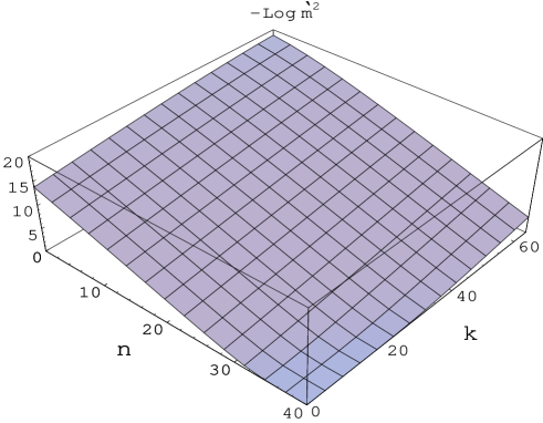
FIG. 1.: Logarithmic plot of the BCM solution field-normalized fermion mass square $\widehat{m}^{2}$ versus couplings $\lambda_{y}=10^{-6+\frac{n}{8}}$ and $\lambda=10^{-9+\frac{k}{8}}$ for $\alpha=\frac{1}{137}$. The numbers in the x-y axes indicate the values of $n$ and $k$, respectively.

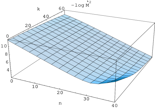
FIG. 2.: Logarithmic plot of the dimensionless scalar square mass $\widehat{M}^{2}$ versus Yukawa and scalar self-interaction couplings. The intervals of the coupling constants used to generate this graph are the same as in Fig.1.

Notice that the fermion mass grows with $\lambda_{y}$ at any given value of $\lambda$. This in turn implies an enhancement of the fermion mass as compared to its value within QED. While in QED the largest mass was no more than $\sim 10^{-10}\surd 2eB$ [2], here the mass surpass this value in the majority of the parameter space in at least 5 orders of magnitude.

It is because of such a significant enhancement of the dynamically generated mass in the presence of scalars, that the magnetic catalysis could play an important role in realistic applications of the HY model. The region of large $\lambda_{y}$, large $\lambda$, where the results are quite reliable, is the most interesting for applications to the electroweak theory, since the values of the coupling constants in that section include the value of the scalar self-couplings consistent with current experimental limits for the Higgs mass, as well as the Yukawa coupling of the top quark.

To finish this subsection, let us consider the behavior of the self energy with the momentum. In Fig. 3 we have plotted the self energy solution (44) as a function of the momentum for fixed values of the couplings. As can be seen, $\sum$ decreases very quickly with the momentum. This behavior is in good agreement with the linearization used in Eq.(34). It also justifies the ultraviolet cutoff at $\surd 2eB$ that was imposed on the integrals appearing in the gap equation (28) and the scalar minimum (24), since, as seen here, the main contribution to the integrals comes from the deep infrared region.

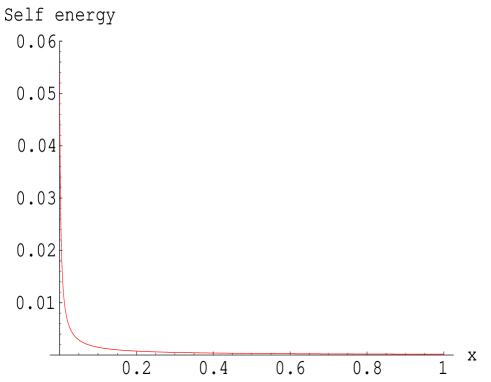
FIG. 3.: Self energy versus momentum squared for $\lambda_{y}=10^{-1}$ and $\lambda=10^{-2}$

C Comparison Between the BCMA and the CMA Solutions

To find the region of reliability of the CMA we have to determine the values of the couplings for which the two approximations give rise to the same mass solutions. With this aim we compare the BCMA equations (57)-(58) with the corresponding CMA equations

$$\widehat{m}=\frac{2}{3}\lambda_{y}\varphi_{c}+\frac{\nu^{2}}{2}\widehat{m}\ln^{2}\frac{1}{\widehat{m}^{2}}$$ (59)

$$\widehat{\varphi}^{3}_{c}=\frac{3\lambda_{y}}{2{\pi}^{2}\lambda}\widehat{m}\ln\frac{1}{\widehat{m}^{2}},$$ (60)

that were previously found in Ref. [13].

Eqs. (59)-(60) look very different from their BCMA counterpart: Eqs. (57)-(58). There is no reason to anticipate that the solutions of both sets of equations will coincide in all the parameter space. Combining Eqs. (59)-(60) we obtain

$$\frac{1}{\widehat{m}^{2}}\ln\frac{1}{\widehat{m}^{2}}=\frac{9\lambda\pi^{2}}{4\lambda^{4}_{y}}[1-\frac{1}{2}\overline{\nu}^{2}ln^{2}\frac{1}{\widehat{m}^{2}}]^{3},$$ (61)

From (61) we see that since $\widehat{m}^{2}$ has to be positive, the consistency of the CMA solution requires $\frac{1}{2}\overline{\nu}^{2}ln^{2}\frac{1}{\widehat{m}^{2}}<1$, which is equivalent to have $t<1.4$. Below, we will numerically check that this condition is indeed always satisfied.

To compare the BCMA and CMA solutions we will explore whether there is a condition under which the CMA and BCMA equations reduce to an identical set. To this end, let us assume that $\overline{\nu}ln\frac{1}{\widehat{m}^{2}}\simeq\nu ln\frac{1}{\widehat{m}^{2}}\ll 1$. This restriction allows us to write Eqs. (57)-(58) as

$$\frac{1}{\widehat{m}^{2}}\ln(\frac{1}{\widehat{m}^{2}})=\frac{9\pi^{2}\lambda}{4\lambda_{y}^{4}},$$ (62)

$$\widehat{M}^{2}=\frac{9\lambda}{8\lambda_{y}^{2}}\widehat{m}^{2}$$ (63)

respectively. They are exactly the same equations found from (60) and (61), after using $t\ll 1$. Thus, in this limiting case, the BCMA reduces to the CMA, thereby $t\ll 1$ defines a condition of reliability of the CMA.

The explicit region of parameter space where the CMA is reliable can be determined from a numerical plot of the ratio between the CMA and BCMA mass square solutions. To be sure that we are working with consistent masses, we will restrict the couplings to a strip in the ($\lambda_{y}$,$\lambda$) plane, leaving out the corner of Fig. 1, where, as discussed above, the consistency of the approximation breaks down.

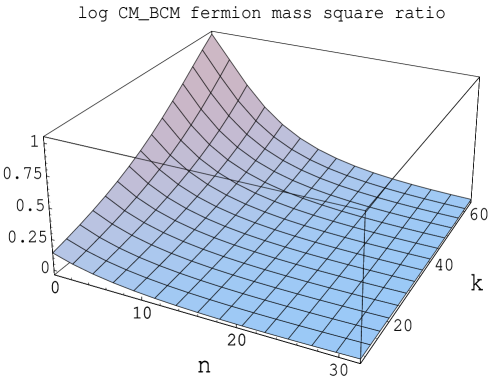
FIG. 4.: $Log(\frac{\widehat{m}_{CM}^{2}}{\widehat{m}_{BCM}^{2}})$ in the region of couplings $10^{-8}<\lambda<10^{-1}$, $10^{-6}<\lambda_{y}<10^{-2}$.

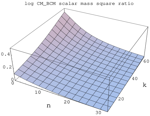
FIG. 5.: $Log(\frac{\widehat{M}_{CM}^{2}}{\widehat{M}_{BCM}^{2}})$ in the region of couplings $10^{-8}<\lambda<10^{-1}$, $10^{-6}<\lambda_{y}<10^{-2}$.

Figs. 4 and 5 show logarithmic plots of the ratio of CMA over BCMA mass square results for fermion and scalar masses respectively, taken in the region of couplings $10^{-8}<\lambda<10^{-1}$, $10^{-6}<\lambda_{y}<10^{-2}$. Both figures display similar behavior of the ratios, characterized by a discernible region of the parameter space, approximately given by $10^{-4}<\lambda<10^{-1}$ and $10^{-6}<\lambda_{y}<10^{-5}$, where a disagreement between BCMA and CMA results is apparent. However, even in this segment, the BCMA and CMA mass squares differ at most in one order of magnitude. Out of this limited region we find very good agreement between BCMA and CMA results, particularly at large $\lambda_{y}$, indicating that this is the most reliable region of the CMA solution within this model.

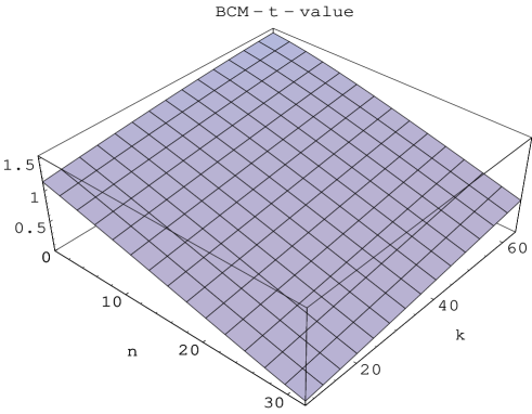
FIG. 6.: The BCM-t-value as a function of $\lambda_{y}=10^{-6+\frac{n}{8}}$ and $\lambda=10^{-9+\frac{k}{8}}$.

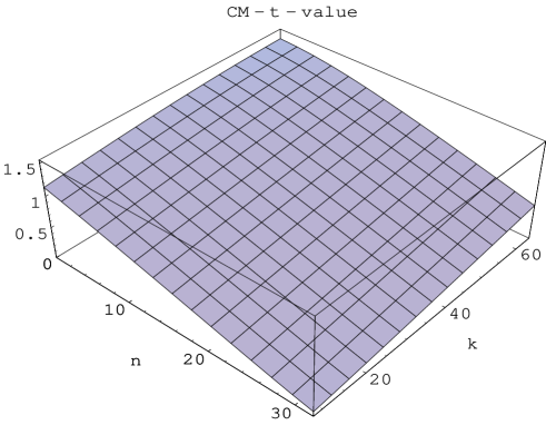
FIG. 7.: The CM-t-value as a function of $\lambda_{y}=10^{-6+\frac{n}{8}}$ and $\lambda=10^{-9+\frac{k}{8}}$.

The above observations are corroborated by the plots of the BCM- and CM- $t$’s, as shown in Figs. 6 and 7 respectively. Both surfaces have similar t-values at equal set of couplings, even when $t\ll 1$ is not satisfied, indicating that, after all, and as already seen in Figs. 4 and 5, the two approximations give rise to very near mass values. Notice that the larger the $\lambda_{y}$’s, the smaller the $t$’s in both approximation, leading to a better agreement between BCMA and CMA results, as expected from our previous analytical considerations. Therefore, although the numerical calculations show that the CMA results are widely reliable, it is in this extreme section of the parameter space where the two approximations totally coincide. From Fig. 7 it is evident that the CM-$t$ never goes over the limiting value of 1.4, so, even in the region of larger discrepancy between the CM and BCM results (large $\lambda$, relatively low $\lambda_{y}$), the CM mass solution remains real, as it should. The curves reflect the fact that the CM-approximation tends to overestimate the mass, because it substitutes in the integrals the self-energy function, which rapidly decreases with momentum, by a constant.

D BCMA in the $\lambda_{y}=0$ Limit (QED case)

We shall discuss now the limiting case $\lambda_{y}=0$ which reduces to (3+1)-dimensional QED with a decoupled self-interacting scalar field. Let us find the solutions for the masses in this case. It is clear from Eq. (24) that no scalar vev, and hence no scalar mass, is generated in this case. The fermion dynamical mass solution can be found from (57) evaluated at $\lambda_{y}=0$. It leads to

$$\tan\left({\verb|t|}\right)=\frac{1}{\nu\epsilon}.$$ (64)

In terms of $\widehat{m}^{2}$, it can be rewritten as follows

$$\widehat{m}^{2}=e^{-\frac{1}{\nu}\arctan(\frac{1}{\nu\epsilon})}$$ (65)

Taking into account that $\nu\epsilon\ll 1$ and using the asymptotic behavior $\arctan(x)\simeq\frac{\pi}{2}-\frac{1}{x}$, we obtain

$$\widehat{m}^{2}=e^{\epsilon}e^{-\pi\surd\frac{\pi}{2\alpha}.}$$ (66)

This result coincides with the BCMA results found for QED within the ladder approximation (see Ref. [2] for details). As known, it is qualitatively very close to its CMA counterpart $\widehat{m}^{2}\simeq e^{-\pi\surd\frac{\pi}{\alpha}}$ [2]. Thus, we are corroborating here the conclusion of the authors of Ref. [2], namely, the reliability of the CMA approach in (3+1)-QED.

It is worth to notice that the dynamical mass behavior is basically affected by the infrared conditions of the self energy, but it is practically indifferent to the ultraviolet boundary condition used in Ref.[2]. This explains why, despite using a momentum cutoff at $\surd 2eB$ and imposing the second boundary condition at $x=1$, we still get in the $\lambda_{y}=0$ case the same result as in [2], where the momentum was allowed to run up to infinity.

IV Concluding Remarks

In this paper we have performed a BCMA study of the magnetically catalyzed fermion and scalar masses in a (3+1)-dimensional Abelian Higgs-Yukawa theory in the presence of a constant magnetic field. Our results show that even in this multiple-coupling theory, the discrepancy between the masses obtained within the CMA and within the more accurate BCMA is not very significant, being the difference in the mass square of at most one order of magnitude. We find that the region where CMA and BCMA results exactly coincide is defined by the condition $\verb|t|=\nu\ln(\frac{1}{\widehat{m}^{2}})\ll 1$.

The BCMA calculations led to fermion masses many orders of magnitude larger than those obtained in the QED case, thereby confirming, within a more accurate approximation, that the Yukawa interactions strengthen the generation of the dynamical fermion mass by several orders of magnitude, a claim done in previous papers [12, 13] based only on CMA results.

As mentioned in the Introduction, a motivation for the inclusion of fermions-scalar interactions in the study of the magnetic catalysis was to find out if this phenomenon could influence the phenomenology of the early universe. A fundamental question here to understand is whether the strengthening of the mass by the fermion-scalar interactions may have any impact in the electroweak phase transition. For this effect to be of any significance for the electroweak physics, a condition has to be met: during the electroweak transition the universe has to be permeated by a primordial magnetic field strong enough as to induce, even at temperatures comparable to the electroweak critical temperature, a modification in the value of the fermion mass.

We should keep in mind that at temperatures below, but close enough, the critical temperature for the electroweak spontaneous symmetry breaking, the fermion masses generated through the Higgs mechanism are very small, since the transition is expected to be either second order or weakly first order. Then, if the magnetic field is much larger than these tiny masses, the fermions will be mainly constrained to their LLL and the MC can be fully operative. However, this is only true if the thermal fluctuations are not as important as to take the fermions out of the LLL. Another way to put this is to say that the critical temperature at which the magnetically induced fermion mass evaporates has to be larger than the electroweak critical temperature.

Magnetic fields may have well been present at the early universe. In fact, there are very plausible arguments favoring the existence of primordial magnetic fields that can serve as the source of the seed fields required to explain the observed magnetic fields in galaxies and clusters of galaxies [23]. The literature on this topic is rich in possible primordial fields generating mechanisms, and many of them can produce very strong fields at and before the electroweak transition [36, 37].

Although the model used in our calculations lacks the complexity of the electroweak theory, it shares some common features with the electromagnetic sector of the electroweak model, and as so we expect that any conclusion drawn within our model can be seen as an indication (even if qualitative) of what the relevance of the effect would be in the electroweak context.

Taking into account that the critical temperature for the vanishing of the magnetically catalyzed fermion mass is typically of the order of the value of the dynamical mass at zero temperature [7, 12], that is $T\sim{m}_{d}(T=0)$, and that a reasonable estimate [36, 37] for the primordial magnetic field at the electroweak scale is $\sim 10^{24}G$, one obtains, for the values of $\lambda_{y}$ and $\lambda$ that gives rise to the largest zero-temperature dynamical mass, that $T_{c}\sim{1GeV}\ll{T}_{ew}\simeq 100GeV$. Hence, no magnetically induced mass would be present at the electroweak temperature because temperature effects override field effects at this scale. Unless new sources of extremely large $B>>T^{2}$ primordial magnetic fields can be identified in the future, these results indicate that the MC has no relevance during the electroweak transition.

Nevertheless, the outcomes of this work may be important for applications of the HY model in situations where magnetic field effects are present at sufficiently low temperatures. We expect that they will be particularly relevant in condensed matter applications. As mentioned in the Introduction, a HY theory has been proposed [22, 26] to describe the observed emergence of a secondary quasiparticle gap in high-$T_{c}$ superconductors at certain doping levels. According to recent experiments [27], the secondary gap can be also triggered by an applied magnetic field. The resemblance of this behavior with the MC is intriguing and deserve a thorough investigation. Such an study, in turn, will require the extension of the results of the present paper to the two-dimensional case in order to make quantitative predictions that can be compared with the experiment.

Acknowledgments

The authors are grateful to V. P. Gusynin for useful discussions. EE is indebted with the Department of Mathematics and Center for Theoretical Physics, MIT, in special with Dan Freedman and Bob Jaffe, for warm hospitality. EJF and VI would like to thank the Institute for Space Studies of Catalonia and the University of Barcelona for their warm hospitality. The work of EE was supported in part by DGI/SGPI (Spain), project BFM2000-0810, and by CIRIT (Catalonia), contract 1999SGR-00257. The work of EJF and VI was supported in part by NSF grant PHY-0070986.

REFERENCES

- [1] V. P. Gusynin, V. A. Miransky, and I. A. Shovkovy, Phys. Rev. Lett. 73 (1994) 3499; Phys. Lett. B 349 (1995) 477.
- [2] V. P. Gusynin, V. A. Miransky, and I. A. Shovkovy, Phys. Rev. D 52 (1995) 4747; Nucl. Phys. B 462 (1996) 249.
- [3] K. G. Klimenko, Z. Phys. C 54 (1992) 323.
- [4] D. K. Hong, Phys. Rev. D 54 (1996) 7879.
- [5] C. N. Leung, Y. J. Ng, and A. W. Ackley, Phys. Rev D 54 (1996) 4181; D.-S Lee, C. N. Leung, and Y. J. Ng, Phys. Rev D 55 (1997) 6504.
- [6] I.A. Shushpanov and A. V. Smilga, Phys. Lett. B 402 (1997) 351.
- [7] V. P. Gusynin and I. A. Shovkovy, Phys. Rev D 56 (1997) 5251.
- [8] D. K. Hong, Phys. Rev. D 57 (1998) 3759.
- [9] V. P. Gusynin, V. A. Miransky, and I. A. Shovkovy, Nucl. Phys. B 563 (1999) 361.
- [10] V. P. Gusynin, E. J. Ferrer and V. de la Incera, Phys. Lett. B 455 (1999) 217.
- [11] E. J. Ferrer and V. de la Incera, Phys. Rev. D 58 (1998) 065008.
- [12] E. J. Ferrer and V. de la Incera, Int. J. Mod. Phys. 14 (1999) 3963.
- [13] E. J. Ferrer and V. de la Incera, Phys. Lett. B 481 (2000) 287.
- [14] V. de la Incera, Proceedings of the International Conference On Quantization, Gauge Theory, And Strings: Conference Dedicated To The Memory Of Professor E.S. Fradkin, pag. 316, edited by A. Semikhatov, M. Vasiliev and V. Zaikin, Scientific World Publ., 5-10 Jun 2000, Moscow, Russia.
- [15] D. Ebert, V. V. Khudyakov, K. G. Klimenko, H. Toki, and V. Ch. Zhukovsky, hep-ph/0108185; V.C. Zhukovsky, V.V. Khudyakov, K.G. Klimenko and D. Ebert, JETP Lett. 74 (2001) 523; D. Ebert, V.V. Khudyakov, K.G. Klimenko and V.Ch. Zhukovsky, Phys.Rev.D 65 (2002) 054024.
- [16] V.A. Miransky and I.A. Shovkovy, Phys.Rev.D66 (2002) 045006.
- [17] V. P. Gusynin, V. A. Miransky, and I. A. Shovkovy, Phys.Rev.D 67 (2003) 107703.
- [18] G. W. Semenoff, I. A. Shovkovy, and L. C. R. Wijewardhana, Mod. Phys. Lett. A 13 (1998) 1143; W. V. Liu, cond-mat/9808134; K. Farakos and N. E. Mavromatos, Phys. Rev. B 57 (1998) 3017; Int. J. Mod. Phys. B 12 (1998) 2475;
- [19] V. Ch. Zhukovsky, K. G. Klimenko, and V. V. Khudyakov, Theor. Math. Phys. 124 (2000) 1132; JETP Lett. 73 (2001) 121.
- [20] E. V. Gorbar, V. P. Gusynin, V. A. Miransky and I. A. Shovkovy, Phys.Rev. B66 (2002) 045108.
- [21] V. P. Gusynin, E. J. Ferrer and V. de la Incera, Mod.Phys.Lett.B 16 (2002) 107; Eur. Phys. Jour. B33 (2003) 397.
- [22] M. Vojta, Y. Zhang, and S. Sachdev,Phys. Rev. Lett. 85 (2000) 4940.
- [23] D. Grasso and H. R. Rubinstein,Phys. Rep. 348 (2001) 163.
- [24] A. C. Durst and P. A. Lee, Phys. Rev.B 62 (2000) 1270.
- [25] T. Valla et al., Science 285 (1999) 2110; Phys. Rev. Lett. 85 (2000) 828.
- [26] D. V. Khveshchenko, and J. Paaske, Phys. Rev. Lett. 86 (2001) 4672.
- [27] Y. Dagan and G. Deutscher,Phys. Rev. Lett. 87 (2001) 177004.
- [28] J. Alexandre, K. Farakos and G. Koutsoumbas, Phys. Rev. D 62 (2000) 105017; Phys. Rev. D 63 (2001) 065015.
- [29] J. Alexandre, K. Farakos and G. Koutsoumbas, Phys. Rev. D 64 (2001) 067702.
- [30] J. M. Cornwall, R. Jackiw and E. Tomboulis, Phys. Rev. D 10 (1974) 2428.
- [31] V.A. Miransky, Dynamical Symmetry Breaking in QFT, (World Scientific, Singapore, 1993).
- [32] V. I. Ritus, Ann. of Phys. (NY) 69 (1972) 555; ZhETF 75 (1978) 1560 (Sov. Phys. JETP 48 (1978) 788); ZhETF 76 (1979) 383.
- [33] V. I. Ritus in Issues in Intense-Field Quantum Electrodynamics, ed. V. L. Ginzburg. Proceedings of P. N. Lebedev Physical Institute, Vol. 111, 5 (1979, Moscow Nauka) (Engl. Transl., V.168, Nova Science, Commack, 1987).
- [34] E. Elizalde, E. J. Ferrer, and V. de la Incera, Annals of Phys. (NY) 295 (2002) 33.
- [35] A. Erderlyi, Higher Transcendental Functions, Vol. 1 (Bateman Manuscript Project, CalTec, McGraw-Hill Book Co.).
- [36] T. Vachaspati, Phys. Lett. B 265 (1991) 258.
- [37] J. Ambjorn and P. Olesen, hep-ph/9304220.