Recent progress in QCD at low energies.

Abstract

The recent results in QCD at low energies are reported. The theoretical analysis of hadronic $\tau$-decay is performed in complex $q^{2}$-plane. The terms of perturbation theory (PT) up to $\alpha^{3}_{s}$ are accounted, the terms of operator product expansion (OPE) – up do dimension 8. The momenta of charmed quark vector current polarization operator are analyzed in 3 loops with account of dimension 4 and 6 OPE terms. The main conclusion is that in the range of low-energy phenomena under consideration PT and OPE are in good agreement with experiment starting from $Q^{2}=-q^{2}\sim 1$ GeV². The values of $\alpha_{s}(m^{2}_{\tau}),\alpha_{s}\langle\overline{q}q\rangle^{2}$, $\langle(\alpha_{s}/\pi)G^{2}\rangle$ and $\overline{m}_{c}(\overline{m}_{c})$ were found.

1 Introduction

The first analysis of QCD at low energies in framework of PT and OPE was performed long ago. The most powerful approach is the method of QCD sum rules [1] (for review of old works see [2], more recent results are reviewed in [3]). In the earlier analysis it was accepted [1], that QCD coupling constant $\alpha_{s}$ is small even at low energies $\alpha_{s}(1$ GeV${}^{2})\approx 0.3$ ($\Lambda^{(3)}_{QCD}\simeq$ 100 MeV) and only first order $\alpha_{s}$ corrections were accounted. Now it is clear, that at low $Q^{2}\sim 1-5$ GeV² $\alpha_{s}(Q^{2})$ is about two times larger, then it was taken in [1]. From the other side, new, more precise experimental data are now available. For these reasons it is necessary the reanalysis of QCD at low energies with account of higher order terms of PT and OPE in comparison with experimental data. In this report I present the results of such analysis.

2 Test of QCD at low energies on the basis of $\tau$-decay data. Determination of $\alpha_{s}(m^{2}_{\tau})$ and of condensate values.

Recently, collaborations ALEPH [4], OPAL [5] and CLEO [6] had measured with a good accuracy the relative probability of hadronic decays of $\tau$-lepton $R_{\tau}=B(\tau\to\nu_{\tau}+hadrons)/B(\tau\to\nu_{\tau}e\overline{\nu}_{e})$, the vector $V$ and axial $A$ spectral functions and the cross section of $e^{+}e^{-}\to hadrons$. Below I present the results of the theoretical analysis of $\tau$-decay data basing on the operator product expansion (OPE) in QCD [7,8]. In the perturbation theory series the terms up to $\alpha^{3}_{s}$ will be taken into account, in OPE – the operators up to dimension 8.

Consider the polarization operator of hadronic currents

$$\Pi^{J}_{\mu\nu}=i~{}\int~{}e^{iqx}\langle TJ_{\mu}(x)J_{\nu}(0)^{{\dagger}}\rangle dx=(q_{\mu}q_{\nu}-q_{\mu\nu}q^{2})\Pi^{(1)}_{J}(q^{2})+q_{\mu}q_{\nu}\Pi^{(0)}_{J}(q^{2}),$$ (1)

$$\mbox{where}~{}~{}~{}~{}J=V,A;~{}~{}~{}V_{\mu}=\bar{u}\gamma_{\mu}d,~{}~{}~{}A_{\mu}=\bar{u}\gamma_{\mu}\gamma_{5}d.$$

The spectral functions measured in $\tau$-decay are imaginary parts of $\Pi^{(1)}_{J}(s)$ and $\Pi^{(0)}_{J}(s)$,   $s=q^{2}$

$$v_{1}/a_{1}(s)=2\pi Im\Pi^{(1)}_{V/A}(s+i0),~{}~{}~{}a_{0}(s)=2\pi Im\Pi^{(0)}_{A}(s+i0)$$ (2)

Functions $\Pi^{(1)}_{V}(q^{2})$ and $\Pi^{(0)}_{A}(q^{2})$ are analytical functions in the $q^{2}$ complex plane with a cut along the right-hand semiaxis starting from $4m^{2}_{\pi}$ for $\Pi^{(1)}_{V}(q^{2})$ and $9m^{2}_{\pi}$ for $\Pi^{(0)}_{A}(q^{2})$. Function $\Pi^{(1)}_{A}(q^{2})$ has kinematical pole at $q^{2}=0$. This is a specific feature of QCD following from chiral symmetry within massless $u$ and $d$ quarks and from its spontaneous violation. The kinematical pole appears due to one-pion state contribution into $\Pi_{A}(q)$, which has the form [7]

$$\Pi^{A}_{\mu\nu}(q)_{\pi}=-\frac{f^{2}_{\pi}}{q^{2}}(q_{\mu}q_{\nu}-q_{\mu\nu}q^{2})-\frac{m^{2}_{\pi}}{q^{2}}q_{\mu}q_{\nu}\frac{f^{2}_{\pi}}{q^{2}-m^{2}_{\pi}}$$ (3)

Consider first the ratio of the total probability of hadronic decays of $\tau$-lepons into states with zero strangeness to the probability of $\tau\to\nu_{\tau}e\overline{\nu}_{e}$. This ratio is given by the equality [9]

$$R_{\tau,V+A}=\frac{B(\tau\to\nu_{\tau}+hadrons_{S=0})}{B(\tau\to\nu_{\tau}e\bar{\nu}_{e})}=$$

$$=6|V_{ud}|^{2}S_{EW}~{}\int\limits^{m^{2}_{\tau}}_{0}~{}\frac{ds}{m^{2}_{\tau}}\Biggl{(}1-\frac{s}{m^{2}_{\tau}}\Biggr{)}^{2}\Biggl{[}\Biggl{(}1+2\frac{s}{m^{2}_{\tau}}\Biggr{)}(v_{1}+a_{1}+a_{0})(s)-2\frac{s}{m^{2}_{\tau}}a_{0}(s)\Biggr{]}$$ (4)

where $|V_{ud}|=0.9735\pm 0.0008$ is the matrix element of the Kabayashi-Maskawa matrix, $S_{EW}=1.0194\pm 0.0040$ is the electroweak correction [10]. Only one-pion state is practically contributing to the last term in (4) and it appears to be small:

$$\Delta R^{(0)}_{\tau}=-24\pi^{2}\frac{f^{2}_{\pi}m^{2}_{\pi}}{m^{4}_{\tau}}=-0.008$$ (5)

Denote

$$\omega(s)\equiv v_{1}+a_{1}+a_{0}=2\pi Im[\Pi^{(1)}_{V}(s)+\Pi{(1)}_{A}(s)+\Pi^{(0)}_{A}(s)]\equiv 2\pi Im\Pi(s)$$ (6)

As follows from eq.(3), $\Pi(s)$ has no kinematical pole, but only right-hand cut. It is convenient to transform the integral in eq.(4) into that over the circle of radius $m^{2}_{\tau}$ in the complex $s$ plane [11]-[13]:

$$R_{\tau,\,V+A}=6\pi i|V_{ud}|^{2}S_{EW}\oint_{|s|=m_{\tau}^{2}}\!{ds\over m_{\tau}^{2}}\left(1-{s\over m_{\tau}^{2}}\right)^{2}\left(1+2{s\over m_{\tau}^{2}}\right)\Pi(s)+\Delta R_{\tau}^{(0)}$$ (7)

Calculate first the perturbative contribution into eq.(7). To this end, use the Adler function $D(Q^{2})$:

$$D(Q^{2})\,\equiv\,-2\pi^{2}\,{d\Pi(Q^{2})\over d\ln{Q^{2}}}\,=\,\sum_{n\geq 0}K_{n}a^{n}\;,\qquad a\equiv{\alpha_{s}\over\pi}\;,\qquad Q^{2}\equiv-s,$$ (8)

the perturbative expansion of which is known up to terms $\sim\alpha^{3}_{s}$. In $\overline{MS}$ regularization scheme $K_{0}=K_{1}=1$,   $K_{2}=1.64$ [14], $K_{3}=6.37$ [15] for 3 flavours and for $K_{4}$ there is the estimate $K_{4}=25\pm 25$ [16]. The renormgroup equation yields

$${da\over d\ln{Q^{2}}}\,=\,-\beta(a)\,=\,-\sum_{n\geq 0}\beta_{n}a^{n+2}\qquad\Rightarrow\qquad\ln{Q^{2}\over\mu^{2}}\,=\,-\,\int_{a(\mu^{2})}^{a(Q^{2})}{da\over\beta(a)},$$ (9)

in the $\overline{MS}$ scheme for three flavours $\beta_{0}=9/4$, $\beta_{1}=4$,   $\beta_{2}=10.06$,   $\beta_{3}=47.23$  [17,18]. Integrating over eq.(8) and using eq.(19) we get

$$\Pi(Q^{2})\,=\,{1\over 2\pi^{2}}\int_{a(\mu^{2})}^{a(Q^{2})}D(a){da\over\beta(a)}$$ (10)

Put $\mu^{2}=m^{2}_{\tau}$ and choose some (arbitrary) value $a(m^{2}_{\tau})$. With the help of eq.(9) one may determine then $a(Q^{2})$ for any $Q^{2}$ and by analytical continuation for any $s$ in the complex plane. Then, calculating (10) find $\Pi(s)$ in the whole complex plane. Substitution of $\Pi(s)$ into eq.(7) determines $R_{\tau}$ for the given $a(m^{2}_{\tau})$ up to power corrections. Thereby, knowing $R_{\tau}$ from experiment it is possible to find the corresponding to it $a(m^{2}_{\tau})$. Note, that with such an approach there is no need to expand the nominator in eqs.(9),(10) in the inverse powers of $lnQ^{2}/\mu^{2}$. Particularly, there is no expansion on the right-hand semiaxis in powers of the parameter $\pi/ln(Q^{2}/\mu^{2})$, which is not small in the investigated region of $Q^{2}$. Advantages of transformation of the integral over the real axis (4) in the contour integral are the following. It can be expected that the applicability region of the theory presented as perturbation theory (PT) + operator expansion (OPE) in the complex $s$-plane is off the shadowed region in Fig.1. It is evident that at positive and comparatively small $s$ PT+OPE do not work. At negative $s=-Q^{2}$ in $\alpha_{s}$ order a nonphysical pole appears, in higher orders, according with (9) it is replaced by a nonphysical cut, which starts from the point $-Q^{2}_{0}$, determined by the formula

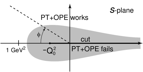
Figure 1: The applicability region of PT and OE in the complex plane $s$. In the dashed region PT + OE does not work.

$$\ln{Q_{0}^{2}\over\mu^{2}}\,=\,-\,\int_{a(\mu^{2})}^{\infty}{da\over\beta(a)}$$ (11)

Integration over the contour allows one to obviate the dashed region in Fig.1 (except for the vicinity of the positive semiaxis, the contribution of which, is suppressed by the factor $(1-\frac{s}{m^{2}_{\tau}})^{2}$ in eq.(7)), i.e. to work in the applicability region of PT+OPE. The OPE terms, i.e., power corrections to polarization operator, are given by the formula:

$$\Pi(s)_{nonpert}=\sum_{n\geq 2}{\left<O_{2n}\right>\over(-s)^{n}}\left(1+c_{n}{\alpha_{s}\over\pi}\right)={\alpha_{s}\over 6\pi\,Q^{4}}\left<G_{\mu\nu}^{a}G_{\mu\nu}^{a}\right>\left(1+{7\over 6}{\alpha_{s}\over\pi}\right)+$$

$$+{128\over 81\,Q^{6}}\,\pi\alpha_{s}\left<\bar{q}q\right>^{2}\left[1+\left({29\over 24}+{17\over 18}\ln{Q^{2}\over\mu^{2}}\right){\alpha_{s}\over\pi}\right]+{\left<O_{8}\right>\over Q^{8}}$$ (12)

($\alpha_{s}$-corrections to the 1-st and 2-d terms in eq.(11) were calculated in [19] and [20], respectively). Contributions of the operator with $d=2$ proportional to $m^{2}_{u}$, $m^{2}_{d}$ and of the condensate $2(m_{u}+m_{d})\langle 0|\bar{q}q|0\rangle$ are neglected. (The latter is of an order of magnitude smaller than the gluonic condensate contribution). When calculating the d=6 term, factorization hypothesis was used. It can be readily seen that d=4 condensates (up to small $\alpha_{s}$ corrections) give no contribution into the integral over contour eq.(7). The contribution from the condensate $\langle O_{8}\rangle$ may be estimated as $|\langle O_{8}\rangle|<10^{-3}GeV^{8}$ and appears to be negligibly small. $R_{\tau,V+A}$ may be represented as

$$R_{\tau,V+A}=3|V_{ud}|^{2}S_{EW}\left(\,1\,+\,\delta_{EW}^{\prime}\,+\,\delta^{(0)}\,+\,\delta^{(6)}_{V+A}\,\right)+\Delta R^{(0)}~{}=$$

$$=~{}3.475\pm 0.022$$ (13)

where $\delta^{\prime}_{em}=(5/12\pi)\alpha_{em}(m^{2}_{\tau})=0.001$ is electromagnetic correction [21], $\delta^{(6)}_{A+V}=-(5\pm 2)\cdot 10^{-3}$ is the contribution of d=6 condensate (see below) and $\delta^{(0)}$ is the PT correction. The right-hand part presents the experimental value obtained as a difference between the total probability of hadronic decays $R_{\tau}=3.636\pm 0.021$ [22] and the probability of decays in states with the strangeness $S=-1~{}~{}R_{\tau,s}=0.161\pm 0.007$ [23,24]. For perturbative correction it follows from eq.(13)

$$\delta^{(0)}=0.206\pm 0.010$$ (14)

Employing the above described method in ref.[8] the constant $\alpha_{s}(m^{2}_{\tau})$ was found from (14)

$$\alpha_{s}(m^{2}_{\tau})=0.355\pm 0.025$$ (15)

The calculation was made with the account of terms $\sim\alpha^{3}_{\tau}$, the estimate of the effect of the terms $\sim\alpha^{4}_{s}$ is accounted for in the error. May be, the error is underestimated (by 0.010-0.015), since the theoretical and experimental errors were added in quadratures.

I determine now the values of condensates basing on the data [3]-[4] on spectral functions. It is convenient first to consider the difference $\Pi_{V}-\Pi_{A}$, which is not contributed by perturbative terms and there remains only the OPE contribution:

$$\Pi_{V}^{(1)}(s)-\Pi_{A}^{(1)}(s)\,=\,\sum_{D\geq 4}\,{O^{V-A}_{D}\over(-s)^{D/2}}\left(\,1\,+\,c_{D}{\alpha_{s}\over\pi}\,\right)\,$$ (16)

The gluonic condensates contribution falls out in the $V-A$ difference and only the following condensates with d=4,6,8 remain

$$O^{V-A}_{4}=2\,(m_{u}+m_{d})\,<\bar{q}q>\;=\;-\,f_{\pi}^{2}m_{\pi}^{2}$$ (17)

$$O^{V-A}_{6}=2\pi\alpha_{s}\left<\,(\bar{u}\gamma_{\mu}\lambda^{a}d)(\bar{d}\gamma_{\mu}\lambda^{a}u)-(\bar{u}\gamma_{5}\gamma_{\mu}\lambda^{a}d)(\bar{d}\gamma_{5}\gamma_{\mu}\lambda^{a}u)\,\right>=$$

$$=-\,{64\pi\alpha_{s}\over 9}<\bar{q}q>^{2}$$ (18)

$$O^{V-A}_{8}=8\pi\alpha_{s}\,m_{0}^{2}<\bar{q}q>^{2}\;,~{}~{}-q\langle 0\mid\overline{q}\sigma_{\mu\nu}\frac{\lambda^{n}}{2}G^{n}_{\mu\nu}q\mid 0\rangle\equiv m^{2}_{0}\langle 0\mid\overline{q}q\mid 0\rangle$$ (19)

In the right-hand of (18) and the first of eq.’s (19) the factorization hypothesis was used. Calculation of the coefficients at $\alpha_{s}$ in eq.(16) gave $c_{4}=4/3$ [19] and $c_{6}=89/48$ [20]. The value of $\alpha_{s}(m^{2}_{\tau})$ (15) corresponds to $\alpha_{s}(1GeV^{2})=0.60$. Thus, if we take for quark condensate at the normlization point $\mu^{2}=1GeV^{2}$ the value following from Gell-Mann-Oakes-Renner relation at $m_{u}+m_{d}=11.7$ MeV, then vacuum condensates with the account of $\alpha_{s}$-corrections appear to be equal (at $\mu^{2}=1GeV^{2}$):

$$O_{4}=-4.22\cdot 10^{-4}~{}GeV^{4}$$ (20)

$$O_{6}=-3.75\cdot 10^{-3}~{}GeV^{6}$$ (21)

$$O_{8}=2.5\cdot 10^{-3}~{}GeV^{8}$$ (22)

(In what follows, indeces $V-A$ will be omitted and $O_{D}$ will mean condensates with the account of $\alpha_{s}$ corrections).

Our aim is to compare OPE theoretical predictions with experimental data on $V-A$ structure functions measured in $\tau$-decay and the values of $O_{6}$ and $O_{8}$ found from experiment to compare with eqs.(21),(22). Numerical values of $O_{6}$ and $O_{8}$ (21),(22) do not strongly differ. This indicates that OPE asymptotic series (16) at $Q^{2}=-s\sim 1GeV^{2}$ converge badly and, may be, even diverge and the role of higher dimension operators may be essential. Therefore it is necessary to improve the series convergence. The most plausible method is to use Borel transformation. Write for $\Pi^{(1)}_{V}-\Pi^{(1)}_{A}$ the subtractionless dispersion relation

$$\Pi^{(1)}_{V}(s)-\Pi^{(1)}_{A}(s)\,=\,{1\over 2\pi^{2}}\int_{0}^{\infty}{v_{1}(t)-a_{1}(t)\over t-s}\,dt\,+\,{f_{\pi}^{2}\over s}$$ (23)

Put $s=s_{0}^{i\phi}$ ($\phi=0$ on the upper edge of the cut) and make the Borel transformation in $s_{0}$. As a result, we get the following sum rules for the real and imaginary parts of (23):

$$\int_{0}^{\infty}\exp{\!\left({s\over M^{2}}\cos{\phi}\right)}\cos{\!\left({s\over M^{2}}\sin{\phi}\right)}(v_{1}-a_{1})(s)\,{ds\over 2\pi^{2}}\,=\,f_{\pi}^{2}+\,\sum_{k=1}^{\infty}(-)^{k}{\cos{(k\phi)}\,O_{2k+2}\over k!\,M^{2k}}$$ (24)

$$\int_{0}^{\infty}\exp{\!\left({s\over M^{2}}\cos{\phi}\right)}\,\sin{\!\left({s\over M^{2}}\sin{\phi}\right)}(v_{1}-a_{1})(s)\,{ds\over 2\pi^{2}M^{2}}\,=\,\sum_{k=1}^{\infty}(-)^{k}{\sin{(k\phi)}\,O_{2k+2}\over k!\,M^{2k+2}}$$ (25)

The use of the Borel transformation along the rays in the complex plane has a number of advantages. The exponent index is negative at $\pi/2<\phi<3\pi/2$. Choose $\phi$ in the region $\pi/2<\phi<\pi$. In this region, on one hand, the shadowed area in fig.1 in the integrals (24),(25) is touched to a less degree, and on the other hand, the contribution of large $s$, particularly, $s>m^{2}_{\tau}$ , where experimental data are absent, is exponentially suppressed. At definite values of $\phi$ the contribution of some condensates vanishes, what may be also used. In particular, the condensate $O_{8}$ does not contribute to (24) at $\phi=5\pi/6$ and to (25) at $\phi=2\pi/3$, while the contribution of $O_{6}$ to (24) vanishes at $\phi=3\pi/4$. Finally, a well known advantage of the Borel sum rules is factorial suppression of higher dimension terms of OPE. Figs.2,3 presents the results of the calculations of left-hand parts of eqs.(24),(25) on the basis of the ALEPH [1] experimental data comparing with OPE predictions – the right-hand part of these equations.

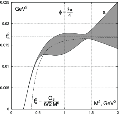
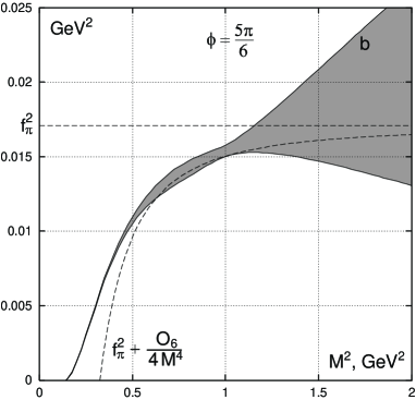
Figure 2: Eq.(24): the left-hand part is obtained basing on the experimental data, the shaded region corresponds to experimental errors; the right-hand part – the theoretical one – is represented by the dotted curve, numerical values of condensates are taken to be equal to the central values of eqs.(26),(27); a) $\phi=3\pi/4$,  b) $\phi=5\pi/6$.

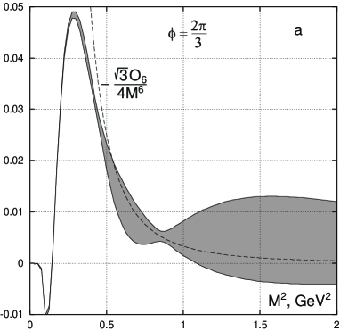
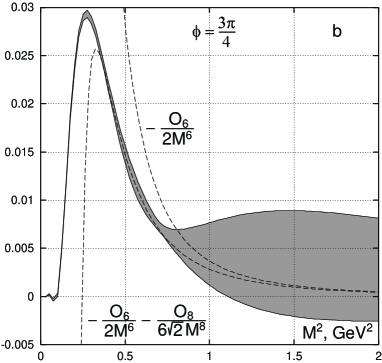
Figure 3: The same for eq.(53): a) $\phi=2\pi/3$,   b) $\phi=3\pi/4$.

The experimental data are best described at the values [7]

$$O_{6}=-(6.8\pm 2.1)\cdot 10^{-3}~{}GeV^{6}$$ (26)

$$O_{8}=-(7\pm 4)\cdot 10^{-3}~{}GeV^{8}$$ (27)

When estimating errors in (26),(27), an uncertainty of higher dimension operator contribution was taken into account in addition to experimental errors. (For details – see [7]).

As is seen from the figures, at these values of condensates a good agreemeent with experiment starts rather early – at $M^{2}>0.5GeV^{2}$. The values (26),(27) are by a factor of 1.5-2 larger than (21),(22). As was discussed above, the accuracy of (21),(22) is of order 50$\%$. Therefore, the most plausible is that the real value of condensates $O_{6},O_{8}$ is somewhere close to the lower edge of errors in (26),(27).

Consider now the polarization operator $\Pi(s)$ defined in (6) and condensates entering OPE for $\Pi(s)$ (see (12)). In principle, the perturbative terms contribute to chirality conserving condensates. If we will follow the separation method of perturbative and nonperturbative contribution by introducing infrared cut-off [25,26], then such a contribution would really appear due to the region of virtualities smaller than $\mu^{2}$. In the present paper, according to [8], an another method is exploited, when the $\beta$-function is expanded only in the number of loops, (see eq.(10) and the text after it) but not in $1/lnQ^{2}$. So, the dependence of condensates on the normalization point $\mu^{2}$ is determined only by perturbative corrections, as is seen in (12). Condensates determined in such a way may be called $n$-loop ones (in the given case – 3-loop). Consider the Borel transformation of the sum $\Pi(s)_{pert}+\Pi(s)_{nonpert}$ where $\Pi(s)_{pert}$ is given by eq.(10), and $\Pi(s)_{nonpert}$ – by eq.(12). Fig.4 presents the results of 3-loop calculation for two values of $\alpha_{s}(m^{2}_{\tau})$ – 0.355 and 0.330. The widths of the bands correspond to theoretical error taken to be equal to the last accounted term $K_{3}a^{2}$ in the Adler function (8). (The same result for the error is obtained if one takes 4 loops in $\beta$-function and puts $K_{4}=50\pm 50$). The dotted line corresponds to the sum of contributions of gluonic condensate $\langle\frac{\alpha_{s}}{\pi}G^{2}\rangle=0.012$ GeV⁴ and $O^{V+A}_{6}$ condensate in (12) with numerical value corresponding to $O^{V-A}_{6}$ (26). The dots with errors present experimental data. (The contribution of the operators $d=4$ and $d=6$ is given separately in the insert).

It is seen that the curve with $\alpha_{s}(m^{2}_{\tau})=0.330$ and condensate contributions can be agreed with experiment, starting from $M^{2}=1.1GeV^{2}$, the agreement being improved at smaller values $\langle 0|\frac{\alpha_{s}}{\pi}G^{2}|0\rangle$ than 0.012 GeV⁴. The curve with $\alpha_{s}(m^{2}_{\tau})=0.355$ with the account of condensates coincides with experiment only at $M^{2}>1.5GeV^{2}$. The same tendency persist for the Borel sum rules taken along the rays in the $s$ complex plane at various $\phi$. Fig.5 gives the sum rule for $\phi=5\pi/6$. From consideration of this and of other sum rules there follows the estimation for gluonic condensate:

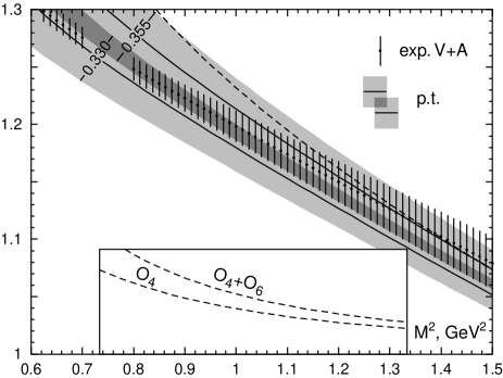
Figure 4: The results of the Borel transformation of $V+A$ correlator for two values $\alpha_{s}(m^{2}_{\tau}=0.355$ and $\alpha_{s}(m^{2}_{\tau})=0.330$. The widths of the bands correspond to PT errors, dots with errors – experimental data. The dotted curve is the sum of the perturbative contribution at $\alpha_{s}(m^{2}_{\tau})=0.330$ and $O_{4}$,  $O_{6}$ condensates.

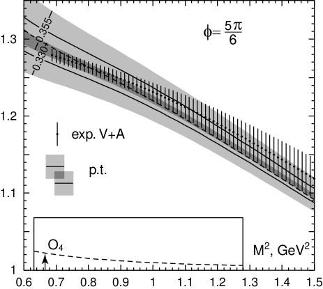
Figure 5: The result of the Borel transformation along the ray at $\phi=5\pi/6$. The dotted line corresponds to the central value of gluonic condensate (56), added to the PT curve with $\alpha_{s}(m^{2}_{\tau})=0.330$.

$$\langle 0\mid\frac{\alpha_{s}}{\pi}G^{a}_{\mu\nu}G^{a}_{\mu\nu}\mid 0\rangle=0.006\pm 0.012~{}GeV^{4}$$ (28)

The best agreement of the theory with experiment in the low $Q^{2}$ region (up to $\sim 2\%$ at $M^{2}>0.8GeV^{2}$) is obtained at $\alpha_{s}(m^{2}_{\tau})=0.330$ which corresponds to $\alpha_{s}(m^{2}_{z})=0.118$.

It was shown [8], that in the dilute instanton gas appoximation [27] instantons do not practically affect determination of $\alpha_{s}(m^{2}_{\tau})$ and the Borel sum rules. Their effect, however, appears to be considerable and strongly dependent on the value of the instanton radius $\rho_{c}$ in the sum rules obtained by integration over closed contours in the complex plane $s$ at the radii of the contours $s<2GeV^{2}$.

3 Sum rules for charmonium and gluonic condensate.

In this Section the charmonium sum rules are revisited. (In what follows I formulate the main results of [28]).

Consider the polarization operator of charmed vector currents

$$i\int dx\,e^{iqx}\left<\,TJ_{\mu}(x)J_{\nu}(0)\,\right>\,=\,(\,q_{\mu}q_{\nu}-g_{\mu\nu}q^{2}\,)\,\Pi(q^{2})\;,\qquad J_{\mu}=\bar{c}\gamma_{\mu}c$$ (29)

The dispersion representation for $\Pi(q^{2})$ has the form

$$R(s)\,=\,4\pi\,{\rm Im}\,\Pi(s+i0)\;,\qquad\Pi(q^{2})\,=\,{q^{2}\over 4\pi^{2}}\int_{4m^{2}}^{\infty}\,{R(s)\,ds\over s(s-q^{2})}\;,$$ (30)

where $R(\infty)=1$ in partonic model. In approximation of infinitely narrow widths of resonances $R(s)$ can be written as sums of contributions from resonances and continuum

$$R(s)\,=\,{3\,\pi\over Q_{c}^{2}\,\alpha_{\rm em}^{2}\!(s)}\,\sum_{\psi}m_{\psi}\Gamma_{\psi\to ee}\,\delta(s-m_{\psi}^{2})\,+\,\theta(s-s_{0})$$ (31)

where $Q_{c}=2/3$ is the charge of charmed quarks, $s_{0}$ - is the continuum threshold (in what follows $\sqrt{s_{0}}=4.6GeV$),    $\alpha(s)$ - is the running electromagnetic constant,  $\alpha(m^{2}_{J/\psi})=1/133.6$ Following [1], to suppress the contribution of higher states and continuum we will study the polarization operator moments

$$M_{n}(Q^{2})\equiv{4\pi^{2}\over n!}\left(-{d\over dQ^{2}}\right)^{n}\Pi(-Q^{2})=\int_{4m^{2}}^{\infty}{R(s)\,ds\over(s+Q^{2})^{n+1}}$$ (32)

According to (31) the experimental values of moments are determind by the equality

$$M_{n}(Q^{2})\,=\,{27\,\pi\over 4\,\alpha_{\rm em}^{2}}\sum_{\psi=1}^{6}{m_{\psi}\Gamma_{\psi\to ee}\over(m_{\psi}^{2}+Q^{2})^{n+1}}\,+\,{1\over n(s_{0}+Q^{2})^{n}}$$ (33)

It is reasonable to consider the ratios of moments $M_{n1}(Q^{2})/M_{n2}(Q^{2})$ from which the uncertainty due to error in $\Gamma_{J/\psi\to ee}$ markedly falls out. Theoretical value for $\Pi(q^{2})$ is represented as a sum of perturbative and nonperturbative contributions. It is convenient to express the perturbative contribution through $R(s)$, making use of (30), (32):

$$R(s)\,=\,\sum_{n\geq 0}R^{(n)}(s,\mu^{2})\,a^{n}(\mu^{2})$$ (34)

where $a(\mu^{2})=\alpha_{s}(\mu^{2})/\pi$. Nowadays, three terms of expansion in (34) are known: $R^{(0)}$ [29]  $R^{(1)}$ [30],   $R^{(2)}$ [31]. They are represented as functions of quark velocity $v=\sqrt{1-4m^{2}/s}$,   where $m$ - is the pole mass of quark. Since they are cumbersome, I will not present them here.

Nonperturbative contributions into polarization operator have the form (restricted by d=6 operators):

$$\Pi_{nonpert}(Q^{2})=\frac{1}{(4m^{2})^{2}}\langle 0\mid\frac{\alpha_{s}}{\pi}G^{2}\mid 0\rangle[~{}f^{(0)}(z)+af^{(1)}(z)~{}]+$$

$$+\frac{1}{(4m^{2})^{3}}g^{3}f^{abc}\langle 0\mid G^{a}_{\mu\nu}G^{b}_{\nu\lambda}G^{c}_{\lambda\mu}\mid 0\rangle F(z),~{}~{}z=-\frac{Q^{2}}{4m^{2}}$$ (35)

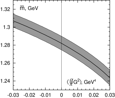
Figure 6: The dependence of $\overline{m}(\overline{m})$ on $\langle 0|\alpha s/\pi)G^{2}|0\rangle$ obtained at $n=10$,  $Q^{2}=0.98\cdot 4m^{2}$ and $\alpha_{s}(Q^{2}+\overline{m}^{2})$.

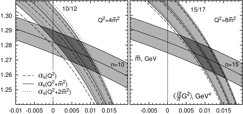
Figure 7: The dependence of $\overline{m}(\overline{m})$ on $\langle 0|(\alpha s/\pi)G^{2}|0\rangle$ obtained from the moments (horizontal bands) and their ratios (vertical bands) at different $\alpha_{s}$. The left-hand figure: $Q^{2}=4\overline{m}^{2}$,   $n=10$,   $M_{10}/M_{12}$; the right-hand figure – $Q^{2}=8\overline{m}^{2}$,   $n=15$,   $M_{15}/M_{17}$.

Functions $f^{(0)}(z)$,   $f^{(1)}(z)$ and $F(z)$ were calculated in [1], [32], [33], respectively. The use of the quark pole mass is, however, inacceptable. So, it is reasonable to turn to $\overline{MS}$ mass $\overline{m}(\mu^{2})$, taken at the point $\mu^{2}=\overline{m}^{2}$. After turning to the $\overline{MS}$ mass $\overline{m}(\overline{m}^{2})$ we

$$n=10\;,\;Q^{2}=4{\bar{m}}^{2}:\qquad{{\bar{M}}^{(1)}\over{\bar{M}}^{(0)}}=0.045\;,\qquad{{\bar{M}}^{(2)}\over{\bar{M}}^{(0)}}=1.136\;,\qquad{{\bar{M}}^{(G,1)}\over{\bar{M}}^{(G,0)}}=-1.673$$ (36)

At $a\sim 0.1$ and at the ratios of moments given by (36) there is a good reason to believe that the PT series well converges. Such a good convergence holds (at $n>5$) only in the case of large enough $Q^{2}$, at $Q^{2}=0$ one does not succeed in finding such $n$, that perturbative corrections, $\alpha_{s}$ corrections to gluonic condensates and the term $\sim\langle G^{3}\rangle$ contribution would be simultaneously small.

It is also necessary to choose the scale - normalization point $\mu^{2}$ where $\alpha_{s}(\mu^{2})$ is taken. In (34)  $R(s)$ is a physical value and cannot depend on $\mu^{2}$. Since, however, we take into account in (34) only three terms, at unsuitable choice of $\mu^{2}$ such $\mu^{2}$ dependence may arise due to neglected terms. At large $Q^{2}$ the natural choice is $\mu^{2}=Q^{2}$. It can be thought that at $Q^{2}=0$ the reasonable scale is $\mu^{2}=\overline{m}^{2}$, though some numerical factor is not excluded in this equality. That is why it is reasonable to take interpolation form

$$\mu^{2}=Q^{2}+\overline{m}^{2},$$ (37)

but to check the dependence of final results on a possible factor at $\overline{m}^{2}$. Equalling theoretical value of some moment at fixed $Q^{2}$ (in the region where $M^{(1)}_{n}$ and $M^{(2)}_{n}$ are small) to its experimental value one can find the dependence of $\overline{m}$ on $\langle(\alpha_{s}/\pi)G^{2}\rangle$ (neglecting the terms $\sim\langle G^{3}\rangle$). Such a dependence for $n=10$ and $Q^{2}/4m^{2}=0.98$ is presented in Fig.6.

To fix both $\overline{m}$ and $\langle(\alpha_{s}/\pi)G^{2}\rangle$ one should, except for moments, take their ratios. Fig.7 shows the value of $\overline{m}$ obtained from the moment $M_{10}$ and the ratio $M_{10}/M_{12}$ at $Q^{2}=4m^{2}$ and from the moment $M_{15}$ and the ratio $M_{15}/M_{17}$ at $Q^{2}=8m^{2}$. The best values of masses of charmed quark and gluonic condensate are obtained from Fig.7:

$${\bar{m}}({\bar{m}}^{2})\,=\,1.275\pm 0.015\,{\rm GeV}\;,\qquad\left<{\alpha_{s}\over\pi}G^{2}\right>\,=\,0.009\pm 0.007\,{\rm GeV}^{4}$$ (38)

Up to now the corrections $\sim\langle G^{3}\rangle$ were not taken into account. It appears that in the region of $n$ and $Q^{2}$ used to find $\overline{m}$ and gluonic condensate they are comparatively small and, practically, not changing $\overline{m}$, increase $\langle(\alpha_{s}/\pi)G^{2}\rangle$ by $10-20\%$ if the term $\sim\langle G^{3}\rangle$ is estimated according to instanton gas model [34] at $\rho_{c}=0.5fm$.

It should be noted that improvement of the accuracy of $\Gamma_{J/\psi\to ee}$ would make it possible to precise the value of gluonic condensate: the widths of horizontal bands in fig.7 are determined mainly just by this error. In particular, this, perhaps, would allow one to exclude the zero value of gluonic condensate, that would be extremely important. Unfortunately, eq.(38) does not allow one to do it for sure. Diminution of theoretical error which determine the width of vertical bands seems to be less real.

4 Conclusion

In this report I compare the results of the recent precise measurements of $\tau$-lepton hadronic decays [4]-[6] with QCD predictions in the low energy region. The perturbative terms up to $\alpha^{3}_{s}$ and the terms of the operator product expansion (OPE) up to d=8 were taken into account. It is shown that QCD with the account of OPE terms agrees with experiment up to $\sim 2\%$ at the values of the complex Borel parameter $|M^{2}|>0.8-1.0GeV^{2}$ in the left-hand semiplane of the complex plane. It was found:
1. The values of the QCD coupling constant $\alpha_{s}(m^{2}_{\tau})=0.355\pm 0.025$ from the total probability of $\tau$-decays and $\alpha_{s}(m^{2}_{\tau})=0.330$ from the sum rules at low energies. (The latter value corresponds to $\alpha_{s}(m^{2}_{z})=0.118$).
2. The value of the quark condensate square (assuming factorization)

$$\alpha_{s}\langle\mid\overline{\psi}\psi\mid 0\rangle^{2}=(2.25\pm 0.70)\cdot 10^{-4}~{}\mbox{GeV}^{6}$$

and of quark-gluon condensate of d=8.
3. The value of gluonic condensate:

a) from the $\tau$-decay data:

$$\langle 0\mid\frac{\alpha_{s}}{\pi}G^{2}\mid 0\rangle=(0.006\pm 0.012)~{}\mbox{GeV}^{4}$$

b) from the sum rules for charmonium

$$\langle 0\mid\frac{\alpha_{s}}{\pi}G^{2}\mid 0\rangle=(0.009\pm 0.007)~{}GeV^{4}$$

It is shown that the sum rules for charmonium are in agreement with experiment when accounting for perturbative corrections $\sim\alpha^{2}_{s}$ and for OPE terms proportional to $\langle(\alpha_{s}/\pi)G^{2}\rangle$ and to $\langle G^{3}\rangle$.

The main conclusion is that in the range of low-energy phenomena under consideration, perturbation theory and operator product expansion are in an excellent agreement with experiment starting from $Q^{2}\sim 1GeV^{2}$.

I am deeply indebted to K.N.Zyablyuk who had made the main calculations in papers [7,8,28], the results of which I used here.

This work was supported by the grants CRDF RP2-2247, INTAS-2000-587 and RFFI 00-02-17808.

References

- [1] M.A.Shifman, A.I.Vainshtein and V.I.Zakharov, Nucl. Phys. 147, 385, 448 (1979).
-
[2]
B.L.Ioffe in: Proc. of the XXII International
Confertence on High Energy Physics, Leipzig, 1984, v.2, p.176
B.L.Ioffe, Lectures in XXIII Cracow School of Physics, Acta Physica Polonica B16, 543 (1984). - [3] P.Colangelo and A.Khodjamirian in: Handbook of QCD, Boris Ioffe Festschrift, ed. by M.Shifman, World Scientific 2001, v.3, p.1495. (1998).
- [4] ALEPH Collaboration, R.Barate et al., Eur.Phys.J.C 4, 409 (1998).
- [5] OPAL Collaboration, K.Ackerstaff et al., Eur.Phys.J.C 7, 571 (1999); G.Abbiendi et al., ibid, 13, 197 (2002).
- [6] CLEO Collaboration, S.J.Richichi et al., Phys.Rev.D 60, 112002 (1999).
- [7] B.L.Ioffe, K.N.Zyablyuk, Nucl.Phys.A 687, 437 (2001).
- [8] B.V.Geshkenbein, B.L.Ioffe, K.N.Zyablyuk, Phys.Rev.D 64, 093009 (2001).
- [9] A.Pich, Proc. of QCD94 Workshop, Monpellier, 1944; Nucl.Phys.B (proc.Suppl) 39, 396 (1995).
- [10] W.J.Marciano, A.Sirlin, Phys.Rev.Lett. 61, 1815 (1988).
- [11] E.Braaten, Phys.Rev.Lett. 60, 1606 (1988); Phys.Rev.D 39, 1458 (1989).
- [12] S.Narison, A.Pich, Phys.Lett.B 211, 183 (1988).
- [13] F.Le Diberder, A.Pich, Phys.Lett.B 286, 147 (1992).
- [14] K.G.Chetyrkin, A.L.Kataev, F.V.Tkachov, Phys.Lett.B 85, 277 (1979); M.Dine, J.Sapirshtein, Phys.Rev.Lett. 43 668 (1979); W.Celmaster, R.Gonsalves, ibid, 44, 560 (1980).
-
[15]
L.R.Surgaladze,
M.A.Samuel, Phys.Rev.Lett. 66, 560 (1991);
S.G.Goryshny, A.L.Kataev, S.A.Larin, Phys.Lett.B 259, 144 (1991). - [16] A.L.Kataev, V.V.Starshenko, Mod.Phys.Lett.A 10, 235 (1995).
- [17] O.V.Tarasov, A.A.Vladimirov, A.Yu.Zharkov, Phys.Lett.B 93, 429 (1980); S.A.Larin, J.A.M.Vermaseren, ibid, 303, 334 (1993).
- [18] T.van Ritbergen, J.A.M.Vermaseren, S.A.Larin, Phys.Lett.B 400, 379 (1997).
- [19] K.G.Chetyrkin, S.G.Gorishny, V.P.Spiridonov, Phys.Lett.B 160, 149 (1985).
- [20] L.-E.Adam, K.G.Chetyrkin, Phys.Lett.B 329, 129 (1994).
- [21] E.Braaten, C.S.Lee, Phys.Rev.D 42, 3888 (1990).
- [22] K.Hagiwara et al., Particle Data Groop, Phys.Rev.D 66, 010001 (2002).
- [23] ALEPH Collaboration, R.Barate et al., Eur.Phys.J.C 11, 599 (1999).
- [24] OPAL Collaboration, G.Abbiendi et al., Eur.Phys.J.C 19, 653 (2001).
- [25] V.A.Novikov, M.A.Shifman, A.I.Vainstein and V.I.Zakharov, Nucl.Phys. B 249, 445 (1985).
- [26] M.A.Shifman, Lecture at 1997 Yukawa International Seminar, Kyoto, 1997, Suppl.Prog.Theor.Phys., 1998, Vol.131, p.1.
- [27] T.Shafer, E.V.Shuryak, Rev.Mod.Phys. 70, 323 (1998).
- [28] B.L.Ioffe, K.N.Zyablyuk, hep-ph/0207183.
- [29] V.B.Berestetsky, I.Ya.Pomeranchuk, JETP 29, 864 (1955).
- [30] J.Schwinger, Particles, Sources, Fields, Addison-Wesley Publ., 1973, V.2.
-
[31]
A.H.Hoang, J.H.Kuhn, T.Teubner,
Nucl.Phys.B 452, 173 (1995);
K.G.Chetyrkin, J.H.Kuhn, M.Steinhauser, Nucl.Phys.B 482, 213 (1996);
K.G.Chetyrkin et al., Nucl.Phys.B 503, 339 (1997);
K.G.Chetyrkin et al., Eur.Phys.J.C 2, 137 (1998). - [32] D.J.Broadhurst et al., Phys.Lett.B 329, 103 (1994).
- [33] S.N.Nikolaev, A.V.Radyushkin, Yad.Fiz. 39, 147 (1984).
- [34] V.A.Novikov, M.A.Shifman, A.I.Vainshtein, V.I.Zakharov, Phys.Let. B86, 347 (1979).