SEMI-NUMERICAL RESUMMATION OF EVENT SHAPES AND JET RATES

Abstract

We describe a numerical procedure to resum multiple emission effects in event shape variables and jet rates.

1 Introduction

Event shape variables (and jet rates) are among the most studied observables in QCD. They are useful both to measure $\alpha_{\mbox{\scriptsize s}}$ [1] and to search for genuine non perturbative (NP) effects [2]. A perturbative (PT) fixed order expansion describes well an event shape rate (the fraction $\Sigma(v)$ of events whose value of the event shape $V$ is less than $v$) in the region $v\sim 1$. In the less inclusive region $v\ll 1$ large logarithms $\alpha_{\mbox{\scriptsize s}}^{m}\ln^{n}v$ arising from incomplete real-virtual cancellations have to be resummed to all orders to give meaning to the PT series [3-7]. In order to fix the scale of $\alpha_{\mbox{\scriptsize s}}$ one needs to control in $\ln\Sigma$ all terms of the form $\alpha_{\mbox{\scriptsize s}}^{n}L^{n+1}$ (leading LL or double DL logarithms) and $\alpha_{\mbox{\scriptsize s}}^{n}L^{n}$ (next-to-leading NLL or single SL logarithms), with $L=\ln 1/v$. It is therefore important to understand the sources of large logarithmic contributions and to find a general way to resum them, at least at NLL level. The aim of the paper is to describe a general procedure to resum SL terms arising from multiple emission effects, which is the most difficult task in any resummation programme.

2 Classification of large logarithms

Leading logarithms originate from soft and collinear gluon radiation and are in general straightforward to resum. SL contributions instead have a variety of sources:

• running of the coupling;

• soft emission at large angles;

• hard collinear splitting;

• multiple emission effects.

The first three contributions can be easily resummed by computing the first order result (in the soft-collinear limit), and exponentiating the answer. The last contribution is the most difficult to address. In the luckiest case (additive observable) it requires only one Laplace transform [3], in more complicated cases one needs to introduce an additional amount of Fourier transforms [4] (which can be as many as five in the thrust minor case [6]). There are situations (thrust major, oblateness) in which an analytical formulation does not even exist at all. It is therefore important to investigate if there is a general method capable to resum SL terms arising from multiple emission effects.

3 Resummation of multiple emission effects

A resummed integrated distribution for a ‘suitable’ (for a definition see [8]) observable $V$ can be written in the form

$$\Sigma(v)=e^{-R(v)}\>{\cal{F}}(R^{\prime})\>,\qquad R^{\prime}=-v\frac{dR}{dv}\>,$$ (1)

where the radiator $R$ builds up the Sudakov form factor obtained by exponentiating the one soft-collinear gluon contribution, while ${\cal{F}}(R^{\prime})$ is a SL function which accounts for multiple emission effects. Suppose that we know the resummed distribution $D_{s}(v_{s})$ of a ‘simple’ variable $V_{s}$. The distribution $D(v)$ of a more complicated observable $V$ is related to $D_{s}(v_{s})$ by:

$$D(v)=v\int\frac{dv_{s}}{v_{s}}P(v|v_{s})\>D_{s}(v_{s})\>,$$ (2)

with $P(v|v_{s})$ the probability of having $V$ equal to $v$ given a value $v_{s}$ for $V_{s}$. The result (2) is quite general. If $V$ and $V_{s}$ have the same DL structure, it can be simplified to give, at SL accuracy:

$$\begin{split}\Sigma(v)=\Sigma_{s}(v)\,{\cal{F}}(R^{\prime})\>,\quad{\cal{F}}(R^{\prime})=\int\frac{dx}{x}x^{-R^{\prime}}p(x,R^{\prime})\>,\quad p\left(\frac{v}{v_{s}},R^{\prime}\right)=vP(v|v_{s})\>.\end{split}$$ (3)

If we now choose $V_{s}(\{k_{i}\})=\max_{i}\{V(k_{i})\}$, the resummation of $\Sigma_{s}(v_{s})$ leads directly to

$$\Sigma_{s}(v_{s})=e^{-R(v_{s})}\>,$$ (4)

so that the function ${\cal{F}}(R^{\prime})$ obtained from (3) coincides with the one introduced in (1).

The effort of any resummation is then to compute $p(x,R^{\prime})$. This can be done numerically with the following Monte Carlo procedure. One starts with a given Born configuration with a fixed number of jets. One then

1. fixes a value $v_{s}$ of the simple observable;

2. generates a soft and collinear emission according to the phase space $R^{\prime}$, with $V(k_{i})<V(k_{i-1})$;

3. if $V(k_{i})<\epsilon\ll 1$ one stops, otherwise goes back to step $I$;

4. given the momentum set $\{k_{i}\}_{i=1,\dots,n}$ one computes the value of the observable $v=V(k_{1},\dots,k_{n})$.

The above procedure gives the probability $P(v|v_{s})$, which can be integrated according to (3) to give the function ${\cal{F}}(R^{\prime})$.

Figure 1: Comparison of the analytical and numerical results for the function ${\cal{F}}(R^{\prime})$ for the thrust and the two broadenings. The lines represent the analytical predictions while the dots are the numerical results.

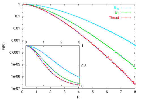
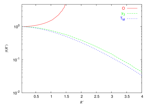
The method is process independent and has been tested in the case of observables for which an analytical resummation is known. For the thrust and the two broadenings $B_{T}$ and $B_{W}$ the results are shown in figure 1. The Monte Carlo procedure reproduces with great precision the function ${\cal{F}}(R^{\prime})$ for these observables. This means that numerical results are truly interchangeable with analytical ones. The method has then been applied [8] to the thrust major $T_{M}$ and the oblateness $O$, for which a resummed prediction did not exist yet, and to the three-jet resolution $y_{3}$ (Durham algorithm [9]), for which only a part of SL contributions had been computed [10] (see figure 2).

Figure 2: The function ${\cal{F}}(R^{\prime})$ for the thrust major $T_{M}$, the oblateness $O$ and the three-jet resolution $y_{3}$.

This new method can then be seen as a first step towards a full automatic resummation of event shapes and jet rates at NLL accuracy.

Acknowledgements

It was a pleasure to carry out this work with Gavin Salam and Giulia Zanderighi. I am also grateful to Matteo Cacciari, Yuri Dokshitzer, Pino Marchesini, Lorenzo Magnea and Graham Smye for helpful comments and suggestions.