ABSTRACT

We derive the general resummed effective Lagrangian for Higgs-mediated flavour-changing neutral-current (FCNC) interactions in the Minimal Supersymmetric Standard Model (MSSM), without resorting to particular assumptions that rely on the squark-mass or the quark-Yukawa structure of the theory. In our derivation we also include the possibility of explicit CP violation through the Cabibbo–Kobayashi–Maskawa mixing matrix and soft supersymmetry-breaking mass terms. The advantages of our resummed FCNC effective Lagrangian are explicitly demonstrated within the context of phenomenologically motivated scenarios. We obtain new testable predictions in the large $\tan\beta$ regime of the theory for CP-conserving and CP-violating observables related to the $K$- and $B$-meson systems, such as $\Delta M_{K,B}$, $\epsilon_{K}$, $\epsilon^{\prime}/\epsilon$, ${\cal B}(B_{d,s}\to\ell^{+}\ell^{-})$ and their associated leptonic CP asymmetries. Finally, based on our resummed FCNC effective Lagrangian, we can identify configurations in the soft supersymmetry-breaking parameter space, for which a kind of a Glashow–Iliopoulos–Maiani-cancellation mechanism becomes operative and hence all Higgs-mediated, $\tan\beta$-enhanced effects on $K$- and $B$-meson FCNC observables vanish.

1 Introduction

The appearance of too large flavour-changing neutral-current (FCNC) interactions of Higgs bosons to fermionic matter is a generic feature of SU(2)${}_{L}\times$U(1)_Y theories with two and more Higgs doublets. Unless there is a symmetry to forbid these Higgs-mediated FCNC interactions to occur in the bare Lagrangian of the model [1], their unsuppressed existence will inevitably lead to predictions for rare processes in the kaon and $B$-meson systems that violate experimental limits by several orders of magnitude [1, 2]. In the minimal realization of softly-broken supersymmetry (SUSY), the Minimal Supersymmetric Standard Model (MSSM), the holomorphicity of the superpotential prevents the occurrence of Higgs-boson FCNCs by coupling the one Higgs-doublet superfield, $\widehat{H}_{1}$, to the down-quark sector, and the other one, $\widehat{H}_{2}$, to the up-quark sector. However, the above holomorphic property of the superpotential is violated by finite radiative (threshold) corrections due to soft SUSY-breaking interactions [3, 4]. As a consequence, Higgs-mediated FCNCs reappear at the one-loop level, but are naturally suppressed for low and intermediate values of $\tan\beta=\langle\widehat{H}_{2}\rangle/\langle\widehat{H}_{1}\rangle$, i.e.  for $\tan\beta\stackrel{{\scriptstyle<}}{{{}_{\sim}}}20$. For larger values of $\tan\beta$, e.g. $\tan\beta\stackrel{{\scriptstyle>}}{{{}_{\sim}}}30$, the FCNCs partially overcome the loop suppression factor $1/(16\pi^{2})$ and become phenomenologically relevant [5, 6], especially for the $K$- and $B$-meson systems.

Recently, the topic of Higgs-boson FCNCs in the large-$\tan\beta$ limit of the MSSM has received much attention [5, 6, 7, 8, 9, 10, 11, 12, 13, 14, 15, 16]. Several approaches have been devised to implement the non-holomorphic finite radiative corrections into the phenomenological analysis of FCNC processes, such as $K^{0}\bar{K}^{0}$ and $B^{0}\bar{B}^{0}$ mixings, $B\to X_{s}\gamma$ and $B_{s}\to\ell^{+}\ell^{-}$. In most cases, however, the suggested approaches to threshold radiative effects involve certain explicit or implicit assumptions pertinent to the squark-mass and the quark-Yukawa structures of the theory, such as the dominance of the top quark in the FCNC transition amplitudes. We term the latter assumption the $t$-quark dominance hypothesis. On the other hand, some of the approaches neglect higher-order terms in the resummation of threshold corrections to $d$-quark Yukawa couplings, which become important in the large-$\tan\beta$ regime of the theory.

In this paper we derive the effective Lagrangian that properly takes into account the resummation of higher-order threshold effects on Higgs-boson FCNC interactions to down quarks. To accomplish this in Section 2, we avoid the imposition of particular assumptions on the structure of the soft squark masses and the quark-Yukawa couplings of the theory. Moreover, we do not rely on specific kinematic approximations to the transition amplitudes, such as the aforementioned $t$-quark dominance hypothesis in the FCNC matrix elements. In our derivation of the effective Lagrangian, we also consider the possibility of CP violation through two sources: (i) the Cabibbo-Kobayashi-Maskawa (CKM) mixing matrix [17] and (ii) the soft SUSY-violating mass terms. As we explicitly demonstrate in Section 3, our resummed FCNC effective Lagrangian gives rise to new testable predictions for CP-conserving as well as CP-violating observables related to the $K$- and $B$-meson systems. In the same section, we qualitatively discuss the implications of $\tan\beta$-enhanced Higgs-mediated interactions for the direct CP-violation parameter $\epsilon^{\prime}/\epsilon$ in the kaon system. Section 4 is devoted to our numerical analysis of a number of $K$- and $B$-meson observables, such as $\Delta M_{K}$, $\epsilon_{K}$, $\Delta M_{B_{d,s}}$, ${\cal B}(B_{d,s}\to\ell^{+}\ell^{-})$ and their associated leptonic CP asymmetries. In particular, based on our resummed FCNC effective Lagrangian, we are able to identify configurations in the soft SUSY-breaking parameter space, for which a kind of a Glashow–Iliopoulos–Maiani-cancellation mechanism (GIM) [18] becomes operative in the Higgs–$d$-quark sector. As a result, all Higgs-mediated, $\tan\beta$-enhanced effects on $K$- and $B$-meson FCNC observables vanish. Finally, Section 5 summarizes our conclusions.

2 Resummed FCNC effective Lagrangian

In this section, we derive the general form for the effective Lagrangian of Higgs-mediated FCNC interactions in the CP-violating MSSM. For this purpose, we also consistently resum the $\tan\beta$-enhanced radiative effects on the $d$-quark Yukawa couplings [7]. First, we analyze a simple soft SUSY-breaking model based on the assumption of minimal flavour violation [6, 10, 13, 14], where the CKM matrix is the only source of flavour and CP violations. We find that even within this minimal framework, the usually neglected $c$-quark contribution to Higgs-mediated FCNC interactions may be competitive to the $t$-quark one in certain regions of the parameter space. After having gained some insight from the above considerations, we then extend our resummed effective Lagrangian approach to more general cases that include a non-universal or hierarchical squark sector as well as CP violation originating from the CKM matrix and the soft SUSY-breaking parameters.

Figure 1: Non-holomorphic radiative effects on the $d$-quark Yukawa couplings induced by (a) gluinos $\tilde{g}$ and (b) charged Higgsinos $\tilde{h}^{-}_{1,2}$.

Before discussing the most general case, let us first consider the following simple form for the effective Yukawa Lagrangian governing the Higgs-mediated FCNC interactions in the quark sector [5, 6]:

$$-{\cal L}_{Y}\ =\ \bar{d}_{R}^{0}\,{\bf h_{d}}\Big{[}\,\Phi^{0*}_{1}\>+\>\Phi^{0*}_{2}\,\Big{(}{\bf\hat{E}_{g}}\>+\>{\bf\hat{E}_{u}}\,{\bf h_{u}^{\dagger}}{\bf h_{u}}\Big{)}\,\Big{]}\,d_{L}^{0}\ +\ \Phi_{2}^{0}\,\bar{u}_{R}^{0}\,{\bf h_{u}}\,u_{L}^{0}\ +\ {\rm H.c.}\,,$$ (2.1)

where $\Phi^{0}_{1,2}$ are the electrically neutral dynamical degrees of freedom of the two Higgs doublets and the superscript ‘0’ on the $d$- and $u$-type quarks denotes fields in the interaction basis. In (2.1), ${\bf h_{d}}$ and ${\bf h_{u}}$ are $3\times 3$-dimensional down- and up-quark Yukawa matrices, and [4, 5, 6]

$${\bf\hat{E}_{g}} = {\bf 1}\,\frac{2\alpha_{s}}{3\pi}\,m_{\tilde{g}}^{*}\mu^{*}\,I(m_{\tilde{d}_{L}}^{2},m_{\tilde{d}_{R}}^{2},|m_{\tilde{g}}|^{2})\;,$$ (2.2)

$${\bf\hat{E}_{u}} = {\bf 1}\,\frac{1}{16\pi^{2}}\,\mu^{*}A_{U}^{*}\,I(m_{\tilde{u}_{L}}^{2},m_{\tilde{u}_{R}}^{2},|\mu|^{2})$$ (2.3)

are finite non-holomorphic radiative effects induced by the diagrams shown in Fig. 1. In the above, the loop integral $I(x,y,z)$ is given by

$$I(x,y,z)\ =\ \frac{xy\ln(x/y)\>+\>yz\ln(y/z)\>+\>xz\ln(z/x)}{(x-y)\,(y-z)\,(x-z)}\ ,$$ (2.4)

with $I(x,x,x)=1/(2x)$. To keep things simple in the beginning, we assume that in (2.2) and (2.3), the bilinear soft SUSY-breaking masses of the squarks, $m^{2}_{\tilde{u}_{L,R}}$, $m^{2}_{\tilde{d}_{L,R}}$, and the trilinear soft Yukawa couplings $A_{U}=A_{u,d}$ are flavour-diagonal and universal at the soft SUSY-breaking scale $M_{\rm SUSY}$. We also neglect the left-right mixing terms $\tilde{u}_{L}$-$\tilde{u}_{R}$ and $\tilde{d}_{L}$-$\tilde{d}_{R}$ in the squark mass matrices. The consequences of relaxing the above assumptions will be discussed later on.

From (2.1), we can easily write down the effective Lagrangian relevant to the effective $d$- and $u$-type quark masses:

$$-{\cal L}_{\rm mass}\ =\ \frac{v_{1}}{\sqrt{2}}\,\bar{d}_{R}^{0}\,{\bf h_{d}}\Big{[}\,{\bf 1}\>+\>\tan\beta\,\Big{(}\,{\bf\hat{E}_{g}}\>+\>{\bf\hat{E}_{u}}\,{\bf h_{u}^{\dagger}}{\bf h_{u}}\,\Big{)}\,\Big{]}\,d_{L}^{0}\ +\ \frac{v_{2}}{\sqrt{2}}\,\bar{u}_{R}^{0}\,{\bf h_{u}}\,u_{L}^{0}\ +\ {\rm H.c.}$$ (2.5)

Our next step is to redefine the quark fields as follows:

$$u_{L}^{0}\ =\ {\bf{\cal U}_{L}^{Q}}\,u_{L}\,,\quad d_{L}^{0}\ =\ {\bf{\cal U}_{L}^{Q}}\,{\bf{V}}\,d_{L}\,,\quad u_{R}^{0}\ =\ {\bf{\cal U}_{R}^{u}}\,u_{R}\,,\quad d_{R}^{0}\ =\ {\bf{\cal U}_{R}^{d}}\,d_{R}\,,$$ (2.6)

where ${\bf{\cal U}_{L}^{Q}}$, ${\bf{\cal U}_{R}^{u}}$, ${\bf{\cal U}_{R}^{d}}$ and ${\bf{V}}$ are 3-by-3 unitary matrices that relate the weak to mass eigenstates of quarks. Evidently, ${\bf{V}}$ is by construction the physical CKM matrix. Substituting (2.6) into (2.5) yields

$$-{\cal L}_{\rm mass}\!\!\! = \!\!\!\frac{v_{1}}{\sqrt{2}}\,\bar{d}_{R}\,{\bf{\cal U}_{R}^{d}}^{\dagger}{\bf h_{d}}{\bf{\cal U}_{L}^{Q}}\,\Big{[}\,{\bf 1}\>+\>\tan\beta\,\Big{(}\,{\bf\hat{E}_{g}}\>+\>{\bf\hat{E}_{u}}|{\bf\hat{h}_{u}}|^{2}\,\Big{)}\,\Big{]}\,{\bf{V}}\,d_{L}\ +\ \frac{v_{2}}{\sqrt{2}}\,\bar{u}_{R}\,{\bf\hat{h}_{u}}\,u_{L}\ +\ {\rm H.c.}$$ (2.7)

$$= \bar{d}_{R}\,{\bf\hat{M}_{d}}\,d_{L}\ +\ \bar{u}_{R}\,{\bf\hat{M}_{u}}\,u_{L}\ +\ {\rm H.c.}\;,$$

where ${\bf\hat{M}_{d}}$ and ${\bf\hat{M}_{u}}$ are the physical $d$- and $u$-quark mass matrices, respectively. Consistency of (2.7) implies

$${\bf\hat{M}_{u}} = \frac{v_{2}}{\sqrt{2}}\,{\bf\hat{h}_{u}}\;,$$ (2.8)

$${\bf{\cal U}_{R}^{d}}^{\dagger}{\bf h_{d}}{\bf{\cal U}_{L}^{Q}} = \frac{\sqrt{2}}{v_{1}}\,{\bf\hat{M}_{d}}{\bf{V}}^{\dagger}\,{\bf\hat{R}}^{-1}\;,$$ (2.9)

with

$${\bf\hat{R}}\ =\ {\bf 1}\>+\>{\bf\hat{E}_{g}}\tan\beta\>+\>{\bf\hat{E}_{u}}\tan\beta\,|{\bf\hat{h}_{u}}|^{2}\;.$$ (2.10)

Notice that (2.9) plays the rôle of a re-defining (renormalization) condition for the $d$-quark Yukawa couplings, in the process of resumming higher-order radiative corrections. Observe also that the matrix ${\bf\hat{R}}$ cannot be zero, as this would result in massless $d$ quarks.

With the help of (2.6) and (2.9), we can now express our original Yukawa Lagrangian (2.1) in terms of the mass eigenstates $d_{L,R}$ and $u_{L,R}$ in a resummed form:

$$-{\cal L}_{Y} = \frac{\sqrt{2}}{v_{1}}\,\bar{d}_{R}\,{\bf\hat{M}_{d}}{\bf{V}}^{\dagger}{\bf\hat{R}}^{-1}\Big{[}\,\Phi_{1}^{0*}\>+\>\Phi_{2}^{0*}\Big{(}{\bf\hat{E}_{g}}\>+\>{\bf\hat{E}_{u}}|{\bf\hat{h}_{u}}|^{2}\Big{)}\,\Big{]}{\bf{V}}\,d_{L}\ +\ \Phi_{2}^{0}\,\bar{u}_{R}{\bf\hat{h}_{u}}u_{L}\ +\ {\rm H.c.}$$ (2.11)

$$= \frac{\sqrt{2}}{v_{2}}\,\Big{(}\tan\beta\,\Phi_{1}^{0*}\>-\>\Phi_{2}^{0*}\Big{)}\,\bar{d}_{R}\,{\bf\hat{M}_{d}}{\bf{V}}^{\dagger}{\bf\hat{R}}^{-1}{\bf{V}}\,d_{L}\ +\ \frac{\sqrt{2}}{v_{2}}\,\Phi_{2}^{0*}\,\bar{d}_{R}\,{\bf\hat{M}_{d}}\,d_{L}$$

$$+\ \Phi_{2}^{0}\,\bar{u}_{R}{\bf\hat{h}_{u}}u_{L}\ +\ {\rm H.c.}$$

In deriving the last equality in (2.11), we have employed the relation: ${\bf\hat{R}}^{-1}({\bf\hat{E}_{g}}+{\bf\hat{E}_{u}}|{\bf\hat{h}_{u}}|^{2})\ =\ ({\bf 1}-{\bf\hat{R}}^{-1})/\tan\beta$.

It is very illuminating to see how the FCNC part of (2.11) compares with the literature, e.g. with that obtained in Ref. [6]. To this end, let us first assume that ${\bf 1}+{\bf\hat{E}_{g}}\tan\beta\neq 0$ and decompose ${\bf\hat{R}}^{-1}$ as follows:

$${\bf\hat{R}}^{-1}\ =\ \frac{{\bf 1}}{{\bf 1}+{\bf\hat{E}_{g}}\tan\beta}\ +\ \chi_{\rm FC}\;,$$ (2.12)

where $\chi_{\rm FC}$ is the diagonal matrix

$$\chi_{\rm FC}\ =\ -\,\frac{{\bf\hat{E}_{u}}\,|{\bf\hat{h}_{u}}|^{2}\,\tan\beta}{({\bf 1}\,+\,{\bf\hat{E}_{g}}\tan\beta)\,{\bf\hat{R}}}\ \;.$$ (2.13)

Making use of the above linear decomposition of ${\bf\hat{R}}^{-1}$ and the unitarity of the CKM matrix in (2.11), the FCNC part of our resummed effective Lagrangian reads

$$-{\cal L}_{\rm FCNC}\!\! = \!\!\frac{\sqrt{2}}{v_{2}}\,\Big{(}\tan\beta\,\Phi_{1}^{0*}\>-\>\Phi_{2}^{0*}\Big{)}\,\bar{d}_{iR}\,m_{d_{i}}\,\bigg{(}\,V_{ti}^{*}\chi_{\rm FC}^{(t)}V_{tj}\>+\>V_{ci}^{*}\chi_{\rm FC}^{(c)}V_{cj}\>+\>V_{ui}^{*}\chi_{\rm FC}^{(u)}V_{uj}\,\bigg{)}d_{jL}\,,$$

where $\chi_{\rm FC}^{(u,c,t)}$ are the diagonal entries of $\chi_{\rm FC}$ and summation over $i,j=d,s,b$ is understood. The term proportional to $\chi_{\rm FC}^{(t)}$ gives the top quark contribution, which is the result of [6] and subsequent articles [10, 13, 14]. However, we should remark here that the frequently-used top-quark dominance approximation cannot be justified from considerations based only on minimal flavour-violation models [6, 10, 13, 14]. In fact, the other terms in (2) and especially the one proportional to $\chi_{\rm FC}^{(c)}$ due to the charm-quark contribution become rather important in the limit ${\bf 1}+{\bf\hat{E}_{g}}\tan\beta\to 0$. In this limit, the singularity in $\chi_{\rm FC}^{(t)}$ is canceled against the singularities of $\chi_{\rm FC}^{(c)}$ and $\chi_{\rm FC}^{(u)}$ as a result of the unitarity of ${\bf{V}}$. In this context, we should note that the limit ${\bf 1}+{\bf\hat{E}_{g}}\tan\beta\to 0$ is not attainable before the theory itself reaches a non-perturbative regime. Requiring that all $d$-quark Yukawa couplings are perturbative, we can estimate the lower bound, $|{\bf 1}+{\bf\hat{E}_{g}}\tan\beta|\stackrel{{\scriptstyle>}}{{{}_{\sim}}}2.5\times 10^{-2}$, for $\tan\beta=50$. Although $|{\bf 1}\>+\>{\bf\hat{E}_{g}}\tan\beta|$ must not vanish in perturbation theory, it can be sufficiently close to zero, so that the $c$-quark contribution becomes competitive with the $t$-quark one.

So far, we have assumed that the radiatively-induced matrices ${\bf\hat{E}_{g}}$ and ${\bf\hat{E}_{u}}$ in the effective Yukawa Lagrangian (2.1) are proportional to the unity matrix. However, this assumption of flavour universality is rather specific. It gets generally invalidated by the mixing of the squark generations, the soft trilinear Yukawa couplings and renormalization-group (RG) running of the soft SUSY-breaking parameters from the unification to the low-energy scale. In this respect, the minimal-flavour-violation hypothesis, although better motivated, should also be viewed as a particular way from minimally departing from universality.

Nevertheless, given that threshold radiative effects on the up sector are negligible, especially for large values of $\tan\beta$, it is straightforward to derive the general resummed form for the Higgs-mediated FCNC effective Lagrangian. Starting from general non-diagonal matrices ${\bf\tilde{E}_{g}}$ and ${\bf\tilde{E}_{u}}$ in (2.1) and following steps very analogous to those from (2.1) to (2.11), we arrive at the same form as in (2.11) for the resummed FCNC effective Lagrangian, but with ${\bf\hat{E}_{g}}$, ${\bf\hat{E}_{u}}$ and ${\bf\hat{R}}$ replaced by

$${\bf{E}_{g}} = {\bf{\cal U}_{L}^{Q}}^{\dagger}{\bf\tilde{E}_{g}}{\bf{\cal U}_{L}^{Q}}\,,\qquad\qquad{\bf{E}_{u}}\ =\ {\bf{\cal U}_{L}^{Q}}^{\dagger}{\bf\tilde{E}_{u}}{\bf{\cal U}_{L}^{Q}}\,,$$ (2.15)

$${\bf{R}} = {\bf 1}\>+\>\tan\beta\,\Big{(}{\bf{E}_{g}}\>+\>{\bf{E}_{u}}\,|{\bf\hat{h}_{u}}|^{2}\>+\>\dots\Big{)}\,,$$ (2.16)

where the ellipses in (2.16) denote additional (generically sub-dominant) threshold effects [20]. Notice that the unitary matrix ${\bf{\cal U}_{L}^{Q}}$ in (2.15), which is only constrained by the relation $|{\bf\hat{h}_{u}}|^{2}={\bf{\cal U}_{L}^{Q}}^{\dagger}{\bf h_{u}^{\dagger}}{\bf h_{u}}{\bf{\cal U}_{L}^{Q}}$, introduces additional non-trivial model dependence in the matrices ${\bf{E}_{g}}$, ${\bf{E}_{u}}$ and ${\bf{R}}$. In other words, the presence of ${\bf{\cal U}_{L}^{Q}}$ reflects the fact that the $3\times 3$-dimensional matrices ${\bf h_{u}^{\dagger}}{\bf h_{u}}$, $m^{2}_{\tilde{u}_{L}}$ and $m^{2}_{\tilde{d}_{L}}$ cannot be diagonalized simultaneously, without generating FCNC couplings in other interactions in the MSSM Lagrangian, e.g. in the $\tilde{W}_{3}$-$u_{L}$-$\tilde{u}_{L}$ and $\tilde{W}^{-}$-$u_{L}$-$\tilde{d}_{L}$ couplings. Moreover, even in minimal flavour-violating scenarios, the $3\times 3$-dimensional matrix ${\bf{R}}$ may generally contain additional radiative effects proportional to ${\bf{\cal U}_{L}^{Q}}^{\dagger}{\bf h_{d}^{\dagger}}{\bf h_{d}}{\bf{\cal U}_{L}^{Q}}$ induced by RG running of the squark masses from the unification to the soft SUSY-breaking scale $M_{\rm SUSY}$. These contributions can be resummed individually by taking appropriately the hermitian square of the modified (2.9) and solving for ${\bf{\cal U}_{L}^{Q}}^{\dagger}{\bf h_{d}^{\dagger}}{\bf h_{d}}{\bf{\cal U}_{L}^{Q}}$. This last step may involve the use of iterative or other numerical methods.

In the general case of a non-universal squark sector, the resummed FCNC couplings of the Higgs bosons to down-type quarks can always be parameterized in terms of a well-defined set of parameters at the electroweak scale. In the weak basis, in which ${\bf{\cal U}_{L}^{Q}}={\bf 1}$, the set of input parameters consists of: (i) the soft squark mass matrices $m^{2}_{\tilde{u}_{L,R}}$, $m^{2}_{\tilde{d}_{L,R}}$ and soft Yukawa-coupling matrices $A_{u,d}$; (ii) the $u$- and $d$-quark masses; (iii) the CKM mixing matrix ${\bf{V}}$.

In our last step in deriving the resummed FCNC effective Lagrangian, we express the Higgs fields $\Phi^{0}_{1,2}$ in terms of their mass eigenstates $H_{1,2,3}$ and the neutral would-be Goldstone boson $G^{0}$ in the presence of CP violation [21]. Following the conventions of [19], we relate the weak to mass eigenstates through the linear transformations:

$$\Phi_{1}^{0} = \frac{1}{\sqrt{2}}\,\Big{[}\,O_{1i}\,H_{i}\ +\ i\,\Big{(}\cos\beta~{}G^{0}\>-\>\sin\beta~{}O_{3i}\,H_{i}\,\Big{)}\,\Big{]}\,,$$

$$\Phi_{2}^{0} = \frac{1}{\sqrt{2}}\,\Big{[}\,O_{2i}\,H_{i}\ +\ i\,\Big{(}\sin\beta~{}G^{0}\>+\>\cos\beta~{}O_{3i}\,H_{i}\,\Big{)}\,\Big{]}\,,$$ (2.17)

where $O_{ij}$ is a 3-by-3 orthogonal matrix that accounts for CP-violating Higgs-mixing effects [22]. If we substitute the weak Higgs fields $\Phi^{0}_{1,2}$ by virtue of (2) into (2.11), we obtain the general resummed effective Lagrangian for the diagonal as well as off-diagonal Higgs interactions to $d$ quarks,

$${\cal L}_{H_{i}\bar{d}d^{\prime}}\ =\ -\,\frac{g_{w}}{2M_{W}}\,\sum_{i=1}^{3}\,H_{i}\>\bar{d}\,\Big{(}\,{\bf\hat{M}_{d}}\,{{\bf g}}_{H_{i}\bar{d}d^{\prime}}^{L}\,P_{L}\ +\ {{\bf g}}_{H_{i}\bar{d}d^{\prime}}^{R}\,{\bf\hat{M}_{d^{\prime}}}P_{R}\,\Big{)}\,d^{\prime}\,,$$ (2.18)

where $P_{L\,(R)}=[1-(+)\,\gamma_{5}]/2$ and

$${{\bf g}}_{H_{i}\bar{d}d^{\prime}}^{L}\!\! = \!\!{\bf{V}}^{\dagger}{\bf{R}}^{-1}{\bf{V}}\,\frac{O_{1i}}{\cos\beta}\ +\ \bigg{(}{\bf 1}\>-\>{\bf{V}}^{\dagger}{\bf{R}}^{-1}{\bf{V}}\,\bigg{)}\,\frac{O_{2i}}{\sin\beta}\ -\ i\,\bigg{(}{\bf 1}\>-\>\frac{1}{\cos^{2}\beta}\,{\bf{V}}^{\dagger}{\bf{R}}^{-1}{\bf{V}}\,\bigg{)}\,\frac{O_{3i}}{\tan\beta}\ ,$$

$${{\bf g}}_{H_{i}\bar{d}d^{\prime}}^{R}\!\! = \!\!\big{(}\,{{\bf g}}_{H_{i}\bar{d}d^{\prime}}^{L}\,\big{)}^{\dagger}\,.$$ (2.19)

The $3\times 3$-dimensional matrix ${\bf{R}}$ in (2), which resums all $\tan\beta$-enhanced finite radiative effects, is given by (2.16). Equation (2.18), along with (2), constitutes the major result of the present paper, which will be extensively used in our phenomenological discussions in Section 3.

Finally, let us summarize the most important properties of the resummed effective Lagrangian (2.18):

• The FCNC interactions in (2.18) are described by $\tan^{2}\beta$-enhanced terms that are proportional to $O_{1i}$ and $O_{3i}$ and to ${\bf{V}}^{\dagger}{\bf{R}}^{-1}{\bf{V}}$ in (2). These $\tan^{2}\beta$-enhanced FCNC terms properly take into account resummation, non-universality in the squark sector and CP-violating effects.

• The resummation matrix ${\bf R}$ controls the strength of the Higgs-mediated FCNC effects. For instance, if ${\bf R}$ is proportional to unity, then a kind of a GIM-cancellation mechanism [18] becomes operative and the Higgs-boson contributions to all FCNC observables vanish identically in this case. Furthermore, as well as the top quark, the other two lighter up-type quarks can give significant contributions to FCNC transition amplitudes, which are naturally included in (2.18) through the resummation matrix ${\bf R}$.

• In the CP-invariant limit of the theory, the effective couplings ${{\bf g}}_{H_{i}\bar{d}d^{\prime}}^{L,R}$ are either pure real or pure imaginary numbers. Moreover, in the limit ${\bf{V}}\to{\bf 1}$, the effective Lagrangian (2.18) of the diagonal Higgs-couplings to down quarks is in excellent agreement with the one presented in [19, 23].

• If $M_{H^{+}}\sim M_{H_{2,3}}\gg M_{H_{1}}$, one can show that $O_{11}\approx\cos\beta$, $O_{21}\approx\sin\beta$ and $O_{31}\approx 0$. In this case, the $H_{1}$-coupling to $d$ quarks becomes SM like and so $H_{1}$-mediated FCNC effects are getting suppressed. Instead, the FCNC couplings of the heavy $H_{2,3}$ bosons to $d$-type quarks retain their $\tan\beta$-enhanced strength in the above kinematic region.

• The one-loop resummed effective Lagrangian (2.18) captures the major bulk of the one-loop radiative effects [24] for large values of $\tan\beta$, e.g.  for $\tan\beta\stackrel{{\scriptstyle>}}{{{}_{\sim}}}40$, and for a soft SUSY-breaking scale $M_{\rm SUSY}$ much higher than the electroweak scale [7]. In addition, (2.18) is only valid in the limit in which the four-momentum of the $d$ quarks and Higgs bosons in the external legs is much smaller than $M_{\rm SUSY}$. This last condition is automatically satisfied in our computations of low-energy FCNC observables.

In the next section, we will study in detail the phenomenological consequences of the $\tan\beta$-enhanced FCNC effects mediated by Higgs bosons on rare processes and CP asymmetries related to the $K$- and $B$-meson systems.

3 Applications to $K$- and $B$-meson systems

We shall now analyze the impact of our resummed effective Lagrangian (2.18) for Higgs-mediated FCNC interactions on representative $K$- and $B$-meson observables. For comprehensive reviews on $K$- and $B$-meson physics, we refer the reader to [25, 26, 27].

3.1 ${\Delta M_{K}}$, ${\epsilon_{K}}$ and $\epsilon^{\prime}/\epsilon$

Our starting point is the effective Hamiltonian for the $\Delta S=2$ interactions,

$$H_{\rm eff}^{\Delta S=2}\ =\ \frac{G_{F}^{2}}{16\pi^{2}}\,M_{W}^{2}\,\sum_{i}\,C_{i}(\mu)\,Q_{i}(\mu)\;,$$ (3.1)

where $G_{F}=1.16639\times 10^{-5}~{}{\rm GeV}^{-2}$ is the Fermi constant, and $C_{i}(\mu)$ are the scale-dependent Wilson coefficients associated to the $\Delta S=2$ quark-dependent operators $Q_{i}$. Note that the CKM matrix elements in (3.1) have been absorbed into the Wilson coefficients. The $\Delta S=2$ operators $Q_{i}$ may be summarized as follows:

$$Q_{1}^{\rm VLL} = (\bar{s}\gamma_{\mu}P_{L}d)(\bar{s}\gamma^{\mu}P_{L}d)\,,\qquad\!Q_{1}^{\rm VRR}\ =\ (\bar{s}\gamma_{\mu}P_{R}d)(\bar{s}\gamma^{\mu}P_{R}d)\,,$$

$$Q_{1}^{\rm LR} = (\bar{s}\gamma_{\mu}P_{L}d)(\bar{s}\gamma^{\mu}P_{R}d)\,,\qquad\ Q_{2}^{\rm LR}\ =\ (\bar{s}P_{L}d)(\bar{s}P_{R}d)\,,$$

$$Q_{1}^{\rm SLL} = (\bar{s}P_{L}d)(\bar{s}P_{L}d)\,,\qquad\qquad Q_{1}^{\rm SRR}\ =\ (\bar{s}P_{R}d)(\bar{s}P_{R}d)\,,$$

$$Q_{2}^{\rm SLL} = (\bar{s}\sigma_{\mu\nu}P_{L}d)(\bar{s}\sigma^{\mu\nu}P_{L}d)\,,\quad Q_{2}^{\rm SRR}\ =\ (\bar{s}\sigma_{\mu\nu}P_{R}d)(\bar{s}\sigma^{\mu\nu}P_{R}d)\;,$$ (3.2)

with $\sigma_{\mu\nu}=\frac{1}{2}[\gamma_{\mu},\gamma_{\nu}]$. Here, much of our discussion and notation follows Ref. [28].

It now proves convenient to decompose both the $K^{0}$-$\bar{K}^{0}$ mass difference ${\Delta M_{K}}$ and the known CP-violating mixing parameter ${\epsilon_{K}}$ into a SM and a SUSY contribution:

$$\Delta M_{K} = M_{K_{L}}\>-\>M_{K_{S}}\ =\ \Delta M_{K}^{\rm SM}+\Delta M_{K}^{\rm SUSY}\;,$$

$$\epsilon_{K} = \epsilon_{K}^{\rm SM}+\epsilon_{K}^{\rm SUSY}\;.$$ (3.3)

To a good approximation, one has

$$\Delta M_{K}^{\rm SM,\,SUSY} = 2\,\Re e\,\langle\bar{K}^{0}|\,H_{\rm eff}^{\Delta S=2}\,|K^{0}\rangle_{\rm SM,\,SUSY}\;,$$ (3.4)

$$\epsilon_{K}^{\rm SM,\,SUSY} = \frac{{\rm exp}(i\pi/4)}{\sqrt{2}\,\Delta M_{K}}\ \Im m\,\langle\bar{K}^{0}|\,H_{\rm eff}^{\Delta S=2}\,|K^{0}\rangle_{\rm SM,\,SUSY}\;.$$ (3.5)

The SUSY contribution to the matrix element $\langle\bar{K}^{0}|H_{\rm eff}^{\Delta S=2}|K^{0}\rangle_{\rm SUSY}$ may be written down as [28, 29]

$$\langle\bar{K}^{0}|\,H_{\rm eff}^{\Delta S=2}\,|K^{0}\rangle_{\rm SUSY} = \frac{G_{F}^{2}}{12\pi^{2}}\,M_{W}^{2}m_{K}F_{K}^{2}\eta_{2}\hat{B}_{K}\,\Big{[}\,\bar{P}_{1}^{\rm VLL}\,\Big{(}\,C_{1}^{\rm VLL}\>+\>C_{1}^{\rm VRR}\,\Big{)}$$ (3.6)

$$+\>\bar{P}_{1}^{\rm LR}\,C_{1}^{\rm LR}\ +\ \bar{P}_{2}^{\rm LR}\,C_{2}^{\rm LR}$$

$$+\>\bar{P}_{1}^{\rm SLL}\,\Big{(}\,C_{1}^{\rm SLL}\>+\>C_{1}^{\rm SRR}\,\Big{)}\ +\ \bar{P}_{2}^{\rm SLL}\,\Big{(}\,C_{2}^{\rm SLL}\>+\>C_{2}^{\rm SRR}\,\Big{)}\,\Big{]}\,,\qquad$$

where $m_{K}=498$ MeV, $F_{K}=160$ MeV and the $\bar{P}$’s are the next-to-leading order (NLO) QCD factors that include the relevant hadronic matrix elements [28, 30, 31, 32, 29]. At the scale $\mu=2$ GeV, they are given by [28]

$$\bar{P}_{1}^{\rm VLL}=0.25\,,\quad\bar{P}_{1}^{\rm LR}=-18.6\,,\quad\bar{P}_{2}^{\rm LR}=30.6\,,\quad\bar{P}_{1}^{\rm SLL}=-9.3\,,\quad\bar{P}_{2}^{\rm SLL}=-16.6\;.$$ (3.7)

On obtaining (3.7), we have used the numerical values: $\eta_{2}=0.57$ and $\hat{B}_{K}=0.85\pm 0.15$.

From studies in the CP-conserving MSSM with minimal flavour violation [29, 10, 14], it is known that for large values of $\tan\beta\stackrel{{\scriptstyle>}}{{{}_{\sim}}}40$, the dominant contribution to $\langle\bar{K}^{0}|H_{\rm eff}^{\Delta S=2}|K^{0}\rangle_{\rm SUSY}$ comes from Higgs-mediated two-loop double penguin (DP) diagrams proportional to $C_{2}^{\rm LR}$. Within the framework of our large-$\tan\beta$-resummed FCNC effective Lagrangian (2.18) that includes CP violation, the Wilson coefficients due to DP graphs are found to be

$$C_{1}^{\rm SLL\,(DP)} = -\,\frac{16\pi^{2}m_{s}^{2}}{\sqrt{2}\,G_{F}M_{W}^{2}}\,\sum_{i=1}^{3}\,\frac{g_{H_{i}\bar{s}d}^{L}\,g_{H_{i}\bar{s}d}^{L}}{M_{H_{i}}^{2}}\;,$$

$$C_{1}^{\rm SRR\,(DP)} = -\,\frac{16\pi^{2}m_{d}^{2}}{\sqrt{2}\,G_{F}M_{W}^{2}}\,\sum_{i=1}^{3}\,\frac{g_{H_{i}\bar{s}d}^{R}\,g_{H_{i}\bar{s}d}^{R}}{M_{H_{i}}^{2}}\;,$$

$$C_{2}^{\rm LR\,(DP)} = -\,\frac{32\pi^{2}m_{s}m_{d}}{\sqrt{2}\,G_{F}M_{W}^{2}}\,\sum_{i=1}^{3}\,\frac{g_{H_{i}\bar{s}d}^{L}\,g_{H_{i}\bar{s}d}^{R}}{M_{H_{i}}^{2}}\;,$$ (3.8)

where the $\tan^{2}\beta$-enhanced couplings $g_{H_{i}\bar{s}d}^{L,R}$ may be evaluated from (2). Note that the DP Wilson coefficients in (3.1) exhibit a $\tan^{4}\beta$-dependence and, although being two-loop suppressed, they become very significant for large values of $\tan\beta\stackrel{{\scriptstyle>}}{{{}_{\sim}}}40$.

In addition to the aforementioned DP contributions due to Higgs-boson exchange graphs, there exist relevant one-loop contributions to $\langle\bar{K}^{0}|H_{\rm eff}^{\Delta S=2}|K^{0}\rangle_{\rm SUSY}$ at large $\tan\beta$: (i) the $t$-$H^{\pm}$ box contribution to $C_{2}^{\rm LR}$ of the two-Higgs-doublet-model (2HDM) type, and (ii) the one-loop chargino-stop box diagram contributing to $C_{1}^{\rm SLL}$. The first contribution (i) becomes significant, up to 10%, only in the kinematic region $M_{H^{\pm}}\approx m_{t}$. In this case, to a good approximation, $C_{1}^{\rm SLL}$ may be given by [29, 10]

$$C_{2}^{\rm LR\,(2HDM)}\approx-\,\frac{2m_{s}m_{d}}{M_{W}^{2}}\,(V_{ts}^{*}V_{td})^{2}\,\tan^{2}\beta\;.$$ (3.9)

Note that the light-quark masses contained in (3.1) and (3.9) are running and are evaluated at the top-quark mass scale, i.e. $m_{s}(m_{t})\simeq 61$ MeV, $m_{d}(m_{t})\simeq 4$ MeV. The second contribution (ii) becomes non-negligible only for small values of the $\mu$-parameter [10, 29], i.e. for $|\mu|\stackrel{{\scriptstyle<}}{{{}_{\sim}}}200$ GeV.

In view of the above discussion, the kinematic parameter range of interest to us is:

$$M_{\rm SUSY},\;\mu\ \gg\ m_{t}\,,\qquad\tan\beta\ \stackrel{{\scriptstyle>}}{{{}_{\sim}}}\ 40\,,$$ (3.10)

including the case $M_{H^{\pm}}\approx m_{t}$, for which the Higgs-mediated DP effects can dominate the $K^{0}$-$\bar{K}^{0}$ transition amplitude. Thus, taking also into account the sub-dominant 2HDM contribution (3.9), formula (3.6) simplifies to

$$\langle\bar{K}^{0}|\,H_{\rm eff}^{\Delta S=2}\,|K^{0}\rangle_{\rm SUSY}\!\! = \!\!4.6\times 10^{-11}{\rm~{}GeV}\ \bigg{(}\,\frac{F_{K}}{160{\rm~{}MeV}}\,\bigg{)}^{2}\,\bigg{(}\,\frac{\eta_{2}}{0.57}\,\bigg{)}\,\bigg{(}\,\frac{\hat{B}_{K}}{0.85}\,\bigg{)}$$ (3.11)

$$\times\,\biggl{[}\,30.6\,\biggl{(}\,C_{2}^{\rm LR\,(DP)}\>+\>C_{2}^{\rm LR\,(2HDM)}\,\biggr{)}\ -\ 9.3\,\biggl{(}\,C_{1}^{\rm SLL\,(DP)}\>+\>C_{1}^{\rm SRR\,(DP)}\,\biggr{)}\,\biggr{]}\,.\qquad$$

Observe that the Wilson coefficients $C_{1}$ and $C_{2}$ contribute with opposite signs to $\langle\bar{K}^{0}|\,H_{\rm eff}^{\Delta S=2}\,|K^{0}\rangle_{\rm SUSY}$. Based on (3.11), we will give numerical estimates of $\Delta M_{K}$ and $\epsilon_{K}$ in Section 4.

We now turn our attention to the computation of the direct CP-violation parameter $\epsilon^{\prime}/\epsilon$ in the kaon system, induced by CP-violating Higgs-mediated FCNC interactions. In the SM, unlike the $Z$-penguin graphs, the Higgs-penguin contribution to $K\to\pi\pi$, which is proportional to the operator

$$Q_{H}\ =\ (\bar{s}P_{L}d)\,\sum_{q=u,d,s}\,(\bar{q}q)\;,$$ (3.12)

has a suppressed Wilson coefficient proportional to $m^{2}_{q}/M^{2}_{H}$, where the SM Higgs-boson mass $M_{H}$ is subject into the experimental bound: $M_{H}\stackrel{{\scriptstyle>}}{{{}_{\sim}}}114$ GeV. One might even think of the possibility that the operator $Q_{H}$ in (3.12), which has enhanced Wilson coefficients for $q=c,b$, mixes with the gluonic and electroweak penguins, as well as with the other basis operators in (3.1). However, as was already pointed out in [33], this is not the case, and so the SM-Higgs penguin effects remain negligible.

The situation changes drastically in the MSSM with explicit CP violation, since the Higgs-boson FCNC couplings to down-type quarks are substantially enhanced by $\tan^{2}\beta$-dependent terms, for large values of $\tan\beta$. Furthermore, besides the CKM phase, the presence of complex soft SUSY-breaking masses with large CP-violating phases may further increase the Higgs-boson FCNC effects on $\epsilon^{\prime}/\epsilon$. In fact, we note that soft CP-odd phases could even be the only source [3] to account for direct CP violation.

To reliably estimate the new SUSY effect on $\epsilon^{\prime}/\epsilon$ due to Higgs-boson FCNC interactions, we normalize each individual contribution with respect to the dominant SM contribution arising from the operator $Q_{6}=\sum_{q=u,d,s}(\bar{s}P_{R}q)(\bar{q}P_{L}d)$ [34, 35], with Wilson coefficient $y_{6}$, viz.

$${\frac{\epsilon^{\prime}}{\epsilon}}\ =\ \biggl{(}{\frac{\epsilon^{\prime}}{\epsilon}}\biggr{)}_{6}\,\Big{(}\,\Omega_{\rm SM}\ +\ \Omega_{\rm SUSY}\ +\ \Omega_{\rm SUSY}^{\rm Higgs}\,\Big{)}\ .$$ (3.13)

In the MSSM with minimal flavour violation, the non-Higgs SUSY contribution $\Omega_{\rm SUSY}$ is small [36]. Sizable contributions may be obtained if one relaxes the assumptions of universality and CP conservation in the squark sector [37, 38].

Here, we compute a novel contribution to $\epsilon^{\prime}/\epsilon$, namely the quantity $\Omega_{\rm SUSY}^{\rm Higgs}$ in (3.13), which entirely originates from Higgs-boson exchange diagrams in the CP-violating MSSM. Based on our resummed FCNC effective Lagrangian (2.18), we obtain in the zero strong-phase approximation

$$\Omega_{\rm SUSY}^{\rm Higgs}\!\! = \!\!2\,\sum_{i=1}^{3}\,\sum_{q=u,d,s}\,\frac{m_{s}\,m_{q}}{M_{H_{i}}^{2}}$$

$$\times\,\Bigg{[}\,\frac{\Im m(g_{H_{i}\bar{s}d}^{L})\,g_{H_{i}\bar{q}q}^{S}}{A^{2}\lambda^{5}\eta}\,\Bigg{(}\,\frac{\langle\pi^{+}\pi^{-}|(\bar{s}P_{L}d)(\bar{q}q)|K^{0}\rangle_{0}}{y_{6}\,\langle\pi^{+}\pi^{-}|Q_{6}|K^{0}\rangle_{0}}\ -\ \frac{1}{|\omega|}\,\frac{\langle\pi^{+}\pi^{-}|(\bar{s}P_{L}d)(\bar{q}q)|K^{0}\rangle_{2}}{y_{6}\,\langle\pi^{+}\pi^{-}|Q_{6}|K^{0}\rangle_{0}}\,\Bigg{)}$$

$$+\,\frac{\Re e(g_{H_{i}\bar{s}d}^{L})\,g_{H_{i}\bar{q}q}^{P}}{A^{2}\lambda^{5}\eta}\,\Bigg{(}\,\frac{\langle\pi^{+}\pi^{-}|(\bar{s}P_{L}d)(\bar{q}\gamma_{5}q)|K^{0}\rangle_{0}}{y_{6}\,\langle\pi^{+}\pi^{-}|Q_{6}|K^{0}\rangle_{0}}\ -\ \frac{1}{|\omega|}\,\frac{\langle\pi^{+}\pi^{-}|(\bar{s}P_{L}d)(\bar{q}\gamma_{5}q)|K^{0}\rangle_{2}}{y_{6}\,\langle\pi^{+}\pi^{-}|Q_{6}|K^{0}\rangle_{0}}\,\Bigg{)}\,\Bigg{]}$$

$$+\,2\sum_{i=1}^{3}\sum_{q=u,d,s}\,\frac{m_{d}\,m_{q}}{M_{H_{i}}^{2}}$$

$$\times\,\Bigg{[}\,\frac{\Im m(g_{H_{i}\bar{s}d}^{R})\,g_{H_{i}\bar{q}q}^{S}}{A^{2}\lambda^{5}\eta}\,\Bigg{(}\,\frac{\langle\pi^{+}\pi^{-}|(\bar{s}P_{R}d)(\bar{q}q)|K^{0}\rangle_{0}}{y_{6}\,\langle\pi^{+}\pi^{-}|Q_{6}|K^{0}\rangle_{0}}\ -\ \frac{1}{|\omega|}\,\frac{\langle\pi^{+}\pi^{-}|(\bar{s}P_{R}d)(\bar{q}q)|K^{0}\rangle_{2}}{y_{6}\,\langle\pi^{+}\pi^{-}|Q_{6}|K^{0}\rangle_{0}}\,\Bigg{)}$$

$$+\,\frac{\Re e(g_{H_{i}\bar{s}d}^{R})\,g_{H_{i}\bar{q}q}^{P}}{A^{2}\lambda^{5}\eta}\,\Bigg{(}\,\frac{\langle\pi^{+}\pi^{-}|(\bar{s}P_{R}d)(\bar{q}\gamma_{5}q)|K^{0}\rangle_{0}}{y_{6}\,\langle\pi^{+}\pi^{-}|Q_{6}|K^{0}\rangle_{0}}\ -\ \frac{1}{|\omega|}\,\frac{\langle\pi^{+}\pi^{-}|(\bar{s}P_{R}d)(\bar{q}\gamma_{5}q)|K^{0}\rangle_{2}}{y_{6}\,\langle\pi^{+}\pi^{-}|Q_{6}|K^{0}\rangle_{0}}\,\Bigg{)}\,\Bigg{]}\,,$$

where the subscripts 0, 2 adhered to the hadronic matrix elements denote the total isospin $I$ of the final states, and $A^{2}\lambda^{5}\eta$ is a CKM combination in the Wolfenstein parameterization, which has the value $A^{2}\lambda^{5}\eta\approx 1.3\times 10^{-4}$ in the SM. Furthermore, for $\Lambda_{\rm QCD}=325$ MeV and $m_{s}=150$ MeV, the SM Wilson coefficient $y_{6}$ and the matrix element of $Q_{6}$ take on the values [35]: $y_{6}=-0.089$ and $\langle\pi^{+}\pi^{-}|Q_{6}|K^{0}\rangle_{0}=-0.35{\rm~{}GeV}^{3}$, respectively. Also, experimental analyses suggest the value $|\omega|=0.045$, approximately yielding the SM contribution $\Omega_{\rm SM}\sim 1$ to $\epsilon^{\prime}/\epsilon$ in (3.13). Finally, the parameters $g^{S,P}_{H_{i}\bar{d}d}$ and $g^{S,P}_{H_{i}\bar{u}u}$ that occur in (3.1) are the diagonal scalar and pseudoscalar couplings of the $H_{i}$ bosons to $u$- and $d$-type quarks [19], whose strengths are normalized to the SM Higgs-boson coupling. These reduced $H_{i}$-couplings are given by

$$g^{S}_{H_{i}\bar{d}d}\! = \!{\textstyle\frac{1}{2}}\,\big{(}\,g^{L}_{H_{i}\bar{d}d}\>+\>g^{R}_{H_{i}\bar{d}d}\,\big{)}\,,\qquad g^{P}_{H_{i}\bar{d}d}\ =\ {\textstyle\frac{i}{2}}\,\big{(}\,g^{L}_{H_{i}\bar{d}d}\>-\>g^{R}_{H_{i}\bar{d}d}\,\big{)}\,,\qquad$$ (3.15)

$$g^{S}_{H_{i}\bar{u}u}\! = \!O_{2i}/\sin\beta\,,\qquad g^{P}_{H_{i}\bar{u}u}\ =\ -O_{3i}\cot\beta\,,$$ (3.16)

where we have neglected the small radiative threshold effects in the up sector.

On the experimental side, the latest world average result for $\Re e(\epsilon^{\prime}/\epsilon)$ is [39]

$$\Re e\bigg{(}\,\frac{\epsilon^{\prime}}{\epsilon}\,\bigg{)}\ =\ (1.66\pm 0.16)\times 10^{-3}\;,$$ (3.17)

at the 1-$\sigma$ confidence level (CL). In the light of the experimental result (3.17) and the discussion given above, we may conservatively require that

$$|\Omega_{\rm SUSY}^{\rm Higgs}|\ \stackrel{{\scriptstyle<}}{{{}_{\sim}}}\ 1\;.$$ (3.18)

The biggest contribution in the sum over quarks in (3.1) comes from the $d$-quark and exhibits the qualitative scaling behaviour

$$\Omega_{\rm SUSY}^{\rm Higgs}\ \simeq\ \frac{2m_{s}m_{d}}{M_{H}^{2}}\,\frac{\tan^{3}\beta}{|\omega|}\,\times\,{\cal O}(1)\;.$$ (3.19)

For instance, for $\tan\beta=50$ and $M_{H}=200$ GeV, (3.19) gives $\Omega_{\rm SUSY}^{\rm Higgs}\simeq 0.1\times{\cal O}(1)$. Obviously, such a contribution is, in principle, non-negligible, but very sensitively depends on the actual values of the new hadronic matrix elements:

$$(Q^{L,R}_{S,P})_{I}\ =\ \langle\pi^{+}\pi^{-}|\,(\bar{s}P_{L,R}d)\,(\bar{q}(1,\gamma_{5})q)\,|K^{0}\rangle_{I}\;,$$ (3.20)

with $I=0,2$. A detailed calculation of the hadronic matrix elements $(Q^{L,R}_{S,P})_{I}$ in (3.20) will be given elsewhere. In Section 4, however, we will present numerical estimates of $\Delta M_{K}$ and $\epsilon_{K}$ within the context of generic soft SUSY-breaking models.

3.2 $\Delta M_{B_{q}}$, $B_{q}\to\ell^{+}\ell^{-}$ and associated CP asymmetries

We start our discussion of a set of observables in the $B$-meson system by first analyzing the $B^{0}_{q}$-$\bar{B}^{0}_{q}$ mass difference, $\Delta M_{B_{q}}$ with $q={s,d}$, in the CP-violating MSSM at large $\tan\beta$. In the applicable limit of equal $B$-meson lifetimes, $\Delta M_{B_{q}}$ may be written as the modulus of a sum of a SM and a SUSY term:

$$\Delta M_{B_{q}}\ =\ 2\,|\langle\bar{B}_{q}^{0}|\,H_{\rm eff}^{\Delta B=2}\,|B^{0}_{q}\rangle_{\rm SM}\ +\ \langle\bar{B}_{q}^{0}|\,H_{\rm eff}^{\Delta B=2}\,|B^{0}_{q}\rangle_{\rm SUSY}|\;,$$ (3.21)

where the effective $\Delta B=2$ Hamiltonian $H_{\rm eff}^{\Delta B=2}$ may be obtained from the $\Delta S=2$ one stated in (3.1), after making the obvious replacements: $s\to b$ and $d\to q$, with $q=d,s$. Proceeding as in Section 3.1, we arrive at analogous closed expressions for the SUSY contributions to the $\Delta B=2$ transition amplitudes:

$$\langle\bar{B}^{0}_{d}|\,H_{\rm eff}^{\Delta B=2}\,|B^{0}_{d}\rangle_{\rm SUSY}\!\! = \!\!1711{\rm~{}ps}^{-1}\Bigg{(}\,\frac{\hat{B}_{B_{d}}^{1/2}\,F_{B_{d}}}{230{\rm~{}MeV}}\,\Bigg{)}^{2}\,\Bigg{(}\,\frac{\eta_{B}}{0.55}\,\Bigg{)}$$

$$\times\,\Big{[}\,0.88\,\Big{(}\,C_{2}^{\rm LR\,(DP)}\>+\>C_{2}^{\rm LR\,(2HDM)}\,\Big{)}\ -\ 0.52\,\Big{(}\,C_{1}^{\rm SLL\,(DP)}\>+\>C_{1}^{\rm SRR\,(DP)}\,\Big{)}\,\Big{]}\;,$$

$$\langle\bar{B}^{0}_{s}|\,H_{\rm eff}^{\Delta B=2}\,|B^{0}_{s}\rangle_{\rm SUSY}\!\! = \!\!2310{\rm~{}ps}^{-1}\Bigg{(}\,\frac{\hat{B}_{B_{s}}^{1/2}\,F_{B_{s}}}{265{\rm~{}MeV}}\,\Bigg{)}^{2}\Bigg{(}\,\frac{\eta_{B}}{0.55}\,\Bigg{)}$$ (3.22)

$$\times\,\Big{[}\,0.88\,\Big{(}\,C_{2}^{\rm LR\,(DP)}\>+\>C_{2}^{\rm LR\,(2HDM)}\,\Big{)}\ -\ 0.52\,\Big{(}\,C_{1}^{\rm SLL\,(DP)}\>+\>C_{1}^{\rm SRR\,(DP)}\,\Big{)}\,\Big{]}\;.\qquad\quad$$

In deriving (3.2), we have also substituted the values determined in [28, 30, 31, 32, 29] for the NLO-QCD factors, along with their hadronic matrix elements at the scale $\mu=4.2$ GeV:

$$\bar{P}_{1}^{\rm LR}\ =\ -0.58\;,\qquad\bar{P}_{2}^{\rm LR}\ =\ 0.88\;,\qquad\bar{P}_{1}^{\rm SLL}\ =\ -0.52\;,\qquad\bar{P}_{2}^{\rm SLL}\ =\ -1.1\;.$$ (3.23)

Moreover, the corresponding Wilson coefficients appearing in (3.2) may be recovered from those in (3.1) and (3.9), after performing the quark replacements mentioned above.

Another observable, which is enhanced at large $\tan\beta$, is the pure leptonic decay of $B$ mesons [5, 6, 8, 9, 10, 11, 12, 13, 14, 15], $\bar{B}^{0}_{q}\to\ell^{+}\ell^{-}$, with $\ell=\mu$, $\tau$. Neglecting contributions proportional to the lighter quark masses $m_{d,s}$, the relevant effective Hamiltonian for $\Delta B=1$ FCNC transitions, such as $b\to q\ell^{+}\ell^{-}$ with $q=d,s$, is given by

$$H_{\rm eff}^{\Delta B=1}\ =\ -\,2\,\sqrt{2}\,G_{F}\,V_{tb}V_{tq}^{*}\,\Big{(}\,C_{S}\,{\cal O}_{S}\ +\ C_{P}\,{\cal O}_{P}\ +\ C_{10}\,{\cal O}_{10}\Big{)}\;,$$ (3.24)

where

$${\cal O}_{S} = \frac{e^{2}}{16\pi^{2}}\,m_{b}\,(\bar{q}P_{R}b)\,(\bar{\ell}\ell)\;,$$

$${\cal O}_{P} = \frac{e^{2}}{16\pi^{2}}\,m_{b}\,(\bar{q}P_{R}b)\,(\bar{\ell}\gamma_{5}\ell)\;,$$

$${\cal O}_{10} = \frac{e^{2}}{16\pi^{2}}\,(\bar{q}\gamma^{\mu}P_{L}b)\,(\bar{\ell}\gamma_{\mu}\gamma_{5}\ell)\;.$$ (3.25)

Employing our resummed FCNC effective Lagrangian (2.18), it is not difficult to compute the Wilson coefficients $C_{S}$ and $C_{P}$ in the region of large values of $\tan\beta$:

$$C_{S} = \frac{2\pi m_{\ell}}{\alpha_{\rm em}}\,\frac{1}{V_{tb}V_{tq}^{*}}\,\sum_{i=1}^{3}\,\frac{g_{H_{i}\bar{q}b}^{R}\,g_{H_{i}\bar{\ell}\ell}^{S}}{M_{H_{i}}^{2}}\ ,$$

$$C_{P} = i\,\frac{2\pi m_{\ell}}{\alpha_{\rm em}}\,\frac{1}{V_{tb}V_{tq}^{*}}\,\sum_{i=1}^{3}\,\frac{g_{H_{i}\bar{q}b}^{R}\,g_{H_{i}\bar{\ell}\ell}^{P}}{M_{H_{i}}^{2}}\ ,$$ (3.26)

while $C_{10}=-4.221$ is the leading SM contribution. In analogy to (3.15), the reduced scalar and pseudoscalar Higgs couplings to charged leptons $g_{H_{i}\bar{\ell}\ell}^{S,P}$ in (3.2) are given by

$$g_{H_{i}\bar{\ell}\ell}^{S}\ =\ \frac{O_{1i}}{\cos\beta}\ ,\qquad g_{H_{i}\bar{\ell}\ell}^{P}\ =\ -\,\tan\beta\,O_{3i}\;,$$ (3.27)

where non-holomorphic vertex effects on the leptonic sector have been omitted as being negligibly small.

With the approximations mentioned above, the branching ratio for the $\bar{B}^{0}_{q}$ meson decay to $\ell^{+}\ell^{-}$ acquires the simple form [9]

$${\cal B}(\bar{B}^{0}_{q}\to\ell^{+}\ell^{-}) =$$

$$\frac{G_{F}^{2}\alpha_{\rm em}^{2}}{16\pi^{3}}\,M_{B_{q}}\tau_{B_{q}}\,|V_{tb}V_{tq}^{*}|^{2}\,\sqrt{1-\frac{4m_{\ell}^{2}}{M_{B_{q}}^{2}}}\ \Bigg{[}\,\Bigg{(}\,1-\frac{4m_{\ell}^{2}}{M_{B_{q}}^{2}}\Bigg{)}\,|F^{q}_{S}|^{2}\ +\ |F_{P}^{q}\>+\>2m_{\ell}F_{A}^{q}|^{2}\,\Bigg{]}\;,$$

where $\tau_{B_{q}}$ is the total lifetime of the $B_{q}$ meson and

$$F_{S,P}^{q}\ =\ -\,\frac{i}{2}\,M_{B_{q}}^{2}F_{B_{q}}\,\frac{m_{b}}{m_{b}+m_{q}}\,C_{S,P}\;,\qquad F_{A}^{q}\ =\ -\,\frac{i}{2}\,F_{B_{q}}\,C_{10}\;.$$ (3.29)

In our numerical estimates, we ignore the contribution from $C_{10}$, as being subdominant in the region of large $\tan\beta$, i.e. for $\tan\beta\stackrel{{\scriptstyle>}}{{{}_{\sim}}}40$, where all Higgs-particle masses are well below the TeV scale. The SM predictions as well as the current experimental bounds pertinent to ${\cal B}(\bar{B}^{0}_{d}\to\ell^{+}\ell^{-})$ can be read off from Table 1 in [41].

In the CP-violating MSSM, an equally important class of observables related to ${\cal B}(\bar{B}^{0}_{d,s}\to\ell^{+}\ell^{-})$ [16] is the one probing possible CP asymmetries that can take place in the same leptonic $B$-meson decays. The leptonic CP asymmetries may shed even light on the CP nature of possible new-physics effects, as the SM prediction for these observables turns out to be dismally small of order $10^{-3}$ [42]. This SM result is a consequence of the fact that the CP-violating phase in $B^{0}$-$\bar{B}^{0}$-mixing parameter $q/p$ is opposite to the one entering the ratio of the amplitudes $\bar{{\cal A}}_{L(R)}(\bar{B}^{0}_{d,s}\to l^{+}_{L(R)}l^{-}_{L(R)})/{\cal A}_{L(R)}({B}^{0}_{d,s}\to l^{+}_{L(R)}l^{-}_{L(R)})$, such that the net CP-violating effect on the observable parameter $\lambda_{L(R)}=(q/p)(\bar{{\cal A}}_{L(R)}/{\cal A}_{L(R)})$ almost cancels out.

There are two possible time-dependent CP asymmetries associated with leptonic $B$-meson decays that are physically allowed:

$${\cal A}_{\rm CP}^{(B_{q}^{0}\to l_{L}^{+}l_{L}^{-})}\ =\ \frac{\int_{0}^{\infty}dt\,\Gamma(B_{q}^{0}(t)\to l_{L}^{+}l_{L}^{-})\>-\>\int_{0}^{\infty}dt\,\Gamma(\bar{B}_{q}^{0}(t)\to l_{R}^{+}l_{R}^{-})}{\int_{0}^{\infty}dt\,\Gamma(B_{q}^{0}(t)\to l_{L}^{+}l_{L}^{-})\>+\>\int_{0}^{\infty}dt\,\Gamma(\bar{B}_{q}^{0}(t)\to l_{R}^{+}l_{R}^{-})}$$ (3.30)

and ${\cal A}_{\rm CP}^{(B_{q}^{0}\to l_{R}^{+}l_{R}^{-})}$, with $L\leftrightarrow R$. Under the assumption that $q/p$ is a pure phase, one finds [42]

$${\cal A}_{\rm CP}^{(B_{q}^{0}\to l_{L}^{+}l_{L}^{-})}\ =\ -\,\frac{2x_{q}\,\Im m\lambda_{q}}{(2\,+\,x_{q}^{2})\>+\>x_{q}^{2}\,|\lambda_{q}|^{2}}\ ,\qquad{\cal A}_{\rm CP}^{(B_{q}^{0}\to l_{R}^{+}l_{R}^{-})}\ =\ -\,\frac{2x_{q}\,\Im m\lambda_{q}}{(2\,+\,x_{q}^{2})\,|\lambda_{q}|^{2}\>+\>x_{q}^{2}}\ ,\quad$$ (3.31)

where $x_{q}=\Delta M_{B_{q}}/\Gamma_{B_{q}}$ and

$$\lambda_{q}\ =\ \frac{M^{q*}_{12}}{|M^{q}_{12}|}\ \Bigg{(}\,\frac{V_{tb}V_{tq}^{*}}{V^{*}_{tb}V_{tq}}\,\Bigg{)}\ \frac{\beta_{l}\,C_{S}\>+\>C_{P}\>+\>2m_{l}C_{10}/(m_{b}M_{B_{q}})}{\beta_{l}\,C_{S}^{*}\>-\>C_{P}^{*}\>-\>2m_{l}C_{10}/(m_{b}M_{B_{q}})}\ .$$ (3.32)

In (3.32), $\beta_{l}=(1-4m_{l}^{2}/M_{B_{q}}^{2})^{1/2}$, $M^{q}_{12}$ is the dispersive part of the $B^{0}_{q}$-$\bar{B}^{0}_{q}$ matrix element, and $C_{S,P}$ are Wilson coefficients given in (3.2). The maximal value that the leptonic CP asymmetries in (3.31) can reach is ${\cal A}_{\rm CP}^{\rm max}=1/\sqrt{2+x_{q}^{2}}$ and is obtained for $\Im m\lambda_{q}=|\lambda_{q}|^{2}$. From current experimental data [43], one may extract the values $x_{d}=0.76$ and $x_{s}\stackrel{{\scriptstyle>}}{{{}_{\sim}}}19$ at the 95% CL, which leads to ${\cal A}_{\rm CP}^{\rm max}(B_{s})\approx 5\%$ and ${\cal A}_{\rm CP}^{\rm max}(B_{d})\approx 62\%$.

Within the framework of our resummed FCNC effective Lagrangian, we also improve earlier calculations [42] of the CP asymmetries by including $B^{0}_{q}$-$\bar{B}^{0}_{q}$ mixing effects through $M^{q*}_{12}/|M^{q}_{12}|$ in (3.32). According to our standard approach of splitting the amplitude into a SM and a MSSM part, we obtain for the SM part

$$M_{12}^{q*\,({\rm SM})}\ =\ \frac{G_{F}^{2}M_{W}^{2}}{12\pi^{2}}\ M_{B_{q}}\eta_{B}\hat{B}_{B_{q}}F_{B_{q}}^{2}\,(V_{tq}V_{tb}^{*})^{2}\,S_{tt}\;,$$ (3.33)

where $S_{tt}\approx 2.38$ is the value of the dominant $m_{t}$-dependent loop function for a top-pole mass $m_{t}=175$ GeV. The SUSY contribution to $M_{12}^{q*\,({\rm SUSY})}=\langle\bar{B}_{d}^{0}|\,H_{\rm eff}^{\Delta B=2}\,|B^{0}_{d}\rangle_{\rm SUSY}$ may be obtained from (3.2).

In the next section, we will present numerical estimates for the $K$- and $B$-meson FCNC observables, based on the analytic expressions derived above.

4 Numerical estimates

In this section, we shall numerically analyze the impact of the $\tan^{2}\beta$-enhanced FCNC interactions on a number of $K$- and $B$-meson observables which were discussed in detail in Sections 3.1 and 3.2, such as ${\Delta M_{K}}$, $\epsilon_{K}$, $\Delta M_{B_{d}}$, $\Delta M_{B_{s}}$, $B_{d}\to\tau^{+}\tau^{-}$, $B_{s}\to\mu^{+}\mu^{-}$ and their associated leptonic CP asymmetries. For our illustrations, we consider two generic low-energy soft SUSY-breaking scenarios, (A) and (B).

In scenario (A), the squark masses are taken to be universal and ${\bf\hat{E}_{g}}$ and ${\bf\hat{E}_{u}}$ are proportional to the unity matrix at the soft SUSY-breaking scale $M_{\rm SUSY}$. The CP-conserving version of this scenario has frequently been discussed in the literature within the context of minimal flavour-violation models, see e.g. [6].

In scenario (B) we assume the existence of a mass hierarchy between the first two generations of squarks and the third generation, namely the first two generations are degenerate and can be much heavier than the third one. In addition, although not mandatory, we assume for simplicity that the model-dependent unitary matrix ${\bf{\cal U}_{L}^{Q}}$ in (2.15) is such that ${\bf{E}_{g}}$ and ${\bf{E}_{u}}$ become diagonal matrices in this scenario. Clearly, in the limit in which all squarks are degenerate, scenario (B) coincides with (A).

In Fig. 2 we give a schematic representation of the generic mass spectrum that will be assumed in our numerical analysis. More explicitly, we fix the charged Higgs-boson $M_{H^{+}}$ to the value $200$ GeV. Since the effect of the gaugino-Higgsino mixing [15, 16] on the resummation matrix ${\bf R}$ can be significantly reduced for $m_{\tilde{W}}\ll\mu$, we ignore this contribution by considering the relatively low value $m_{\tilde{W}}\approx 2m_{t}\ll M_{\rm SUSY}$ in our numerical estimates, with $m_{t}=175$ GeV. As can be seen from Fig. 2, the third-generation soft squark mass $m_{\tilde{t}}$, the $\mu$-parameter, the gluino mass $m_{\tilde{g}}$ and the trilinear soft Yukawa coupling $A_{U}$ are set, for simplicity reasons, to the common soft SUSY-breaking scale $M_{\rm SUSY}$, which is typically taken to be 1 TeV.

The soft squark masses of the other two generations are assumed to be equal to $m_{\tilde{q}}$ in our generic framework. To account for a possible hierarchical difference between the mass scales $m_{\tilde{t}}$ and $m_{\tilde{q}}$, we introduce the so-called hierarchy factor $\rho$, such that $m_{\tilde{q}}=\rho m_{\tilde{t}}=\rho M_{\rm SUSY}$. As has been mentioned above, models of minimal flavour violation correspond to scenario (A) with $\rho=1$. As we will see in detail in Sections 4.1 and 4.2, the predictions for the $K$- and $B$-meson FCNC observables crucially depend on the values of the hierarchy factor $\rho$. Equally important modifications in the predictions are obtained for different values of the soft CP-violating phases $\phi_{g}={\rm arg}\,(m_{\tilde{g}})$ and $\phi_{A_{U}}={\rm arg}\,(A_{U})$. In addition, the $K$- and $B$-meson FCNC observables exhibit a non-trivial dependence on the CKM phase $\delta_{\rm CKM}$, which is varied independently in our figures.

Although we primarily use $\tan\beta=50$ and $M_{H^{+}}=0.2$ TeV as inputs in our numerical analysis, approximate predictions for other values of the input parameters may be obtained by rescaling the numerical estimates by a factor

$$x_{\cal O}\ =\ \bigg{(}\,\frac{\tan\beta}{50}\,\bigg{)}^{n}\>\times\>\bigg{(}\,\frac{0.2~{}{\rm TeV}}{M_{H^{+}}}\,\bigg{)}^{k}\,,$$ (4.1)

where the integers $n$ and $k$ depend on the FCNC observable ${\cal O}$ under study. Such a rescaling proves to be fairly accurate for $\tan\beta\stackrel{{\scriptstyle>}}{{{}_{\sim}}}40$ and $M_{H^{+}}\stackrel{{\scriptstyle>}}{{{}_{\sim}}}150$ GeV, which is the kinematic region of our interest.

4.1 ${\Delta M_{K}}$ and $|\epsilon_{K}|$

The SM effects on ${\Delta M_{K}}$ and $|\epsilon_{K}|$ were extensively discussed in the literature [44], so we will not dwell upon this issue here as well. Instead, we assume that the SM explains well the experimental results for the above two observables [43]:

$$\Delta M_{K}^{\rm exp} = (3.490\pm 0.006)\times 10^{-12}~{}{\rm MeV}\,,$$ (4.2)

$$|\epsilon^{\rm exp}_{K}| = (2.282\pm 0.017)\times 10^{-3}\;.$$ (4.3)

Given the significant uncertainties in the calculation of hadronic matrix elements, however, our approach will be to constrain the soft SUSY-breaking parameters by conservatively requiring that $\Delta M_{K}^{\rm SUSY}$ and $|\epsilon_{K}^{\rm SUSY}|$ do not exceed in size the SM predictions.

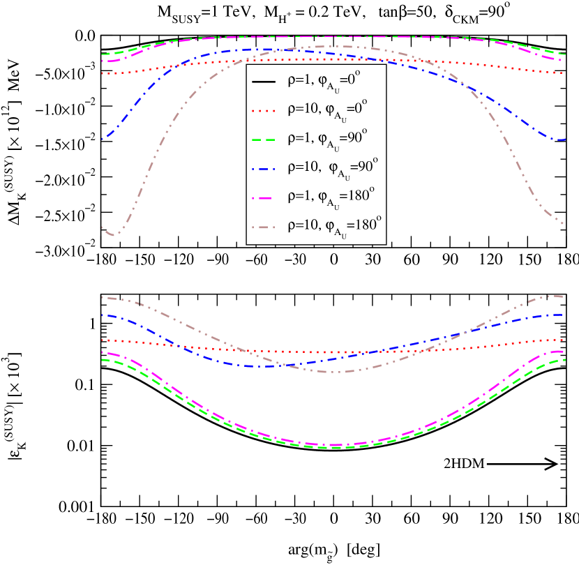
Figure 3: SUSY Higgs-DP contributions to $\epsilon_{K}$ and $\Delta M_{K}$ given in units of $10^{-12}$ MeV and $10^{-3}$, respectively, as functions of the gluino phase ${\rm arg}\,(m_{\tilde{g}})$, for $M_{\rm SUSY}=1$ TeV, $M_{H^{+}}=0.2$ TeV, $\tan\beta=50$ and $\delta_{\rm CKM}=90^{\circ}$. As is shown above, the different curves are obtained for selected values of $\rho$ and $\phi_{A_{U}}$. The size of the 2HDM effect alone on $\epsilon_{K}$ is indicated by an arrow.

To start with, we display in Fig. 3 numerical values for the Higgs-boson DP effects on ${\Delta M_{K}}$ and $|\epsilon_{K}|$ as functions of the gluino phase ${\rm arg}\,m_{\tilde{g}}$, where the hierarchy factor $\rho$ and the phase $\phi_{A_{U}}={\rm arg}\,(A_{t,b})$ of the soft SUSY-breaking trilinear Yukawa couplings assume the discrete values: $(\rho,\ \phi_{A_{U}})=(1,\ 0^{\circ}),\ (10,\ 0^{\circ}),\ (1,\ 90^{\circ}),\ (10,\ 90^{\circ}),(1,\ 180^{\circ}),\ (10,\ 180^{\circ})$. According to our CP-phase conventions [19], $\mu$ is always taken to be positive, while the CKM phase $\delta_{\rm CKM}$ is chosen to its maximal value $90^{\circ}$. The subdominant one-loop 2HDM contribution coming from $W^{\pm}$-$H^{\mp}$ box graphs [cf. (3.9)] has also been indicated by an arrow in Fig. 3. Predictions for $M_{H^{+}}$ and $\tan\beta$ values other than those shown in Fig. 2 may be approximately obtained by multiplying the numerical estimates by a factor $x_{\cal O}=(\tan\beta/50)^{4}\times(0.2~{}{\rm TeV}/M_{H^{+}})^{2}$. We observe in Fig. 3 that the resulting values for $\Delta M_{K}^{\rm SUSY}$ can exceed the experimental error in (4.2) by one order of magnitude, for $\rho=10$ and $|\phi_{A_{U}}|,\ |\phi_{\tilde{g}}|\stackrel{{\scriptstyle>}}{{{}_{\sim}}}90^{\circ}$. For the same inputs, $|\epsilon_{K}^{\rm SUSY}|$ takes on values comparable to the experimentally measured one (4.3). Here, we should stress the fact that universal squark-mass scenarios corresponding to $\rho=1$ can still predict sizeable effects on $\epsilon_{K}$. This non-zero result should be contrasted with the one of the gluino-squark box contributions to ${\Delta M_{K}}$ and $|\epsilon_{K}|$ [45] which do vanish in the limit of strictly degenerate squarks due to a SUSY-GIM-cancellation mechanism.

In our case of Higgs-mediated FCNC observables, however, the situation is slightly different. As we have discussed in Section 2, the size of the FCNC effects is encoded in the flavour structure of the 3-by-3 resummation matrix ${\bf{R}}$. Since ${\bf{R}}$ is diagonal for the scenarios (A) and (B) under consideration, we can expand the $\tan\beta$-enhanced FCNC terms $({\bf{V}}^{\dagger}\,{\bf{R}}^{-1}\,{\bf{V}})_{dd^{\prime}}$ in (2.18) as follows:

$$({\bf{V}}^{\dagger}\,{\bf{R}}^{-1}\,{\bf{V}})_{dd^{\prime}}\ =\ V^{*}_{ud}\,R^{-1}_{u}\,V_{ud^{\prime}}\>+\>V^{*}_{cd}\,R^{-1}_{c}\,V_{cd^{\prime}}\>+\>V^{*}_{td}\,R^{-1}_{t}\,V_{td^{\prime}}\;,$$ (4.4)

where $d$ and $d^{\prime}$ collectively denote all down-type quarks, with $d\neq d^{\prime}$. For the parameters adopted in Fig. 2, the quantities $R^{-1}_{u,c,t}$ can be simplified further to

$$R^{-1}_{u} \approx \bigg{[}\,1\>+\>\bigg{(}\,\frac{\alpha_{s}}{3\pi\rho^{2}}\,e^{-i\phi_{\tilde{g}}}\>+\>\frac{|h_{u}|^{2}}{32\pi^{2}\rho^{2}}\,e^{-i\phi_{A_{U}}}\,\bigg{)}\tan\beta\,\bigg{]}^{-1}\;,$$

$$R^{-1}_{c} \approx \bigg{[}\,1\>+\>\bigg{(}\,\frac{\alpha_{s}}{3\pi\rho^{2}}\,e^{-i\phi_{\tilde{g}}}\>+\>\frac{|h_{c}|^{2}}{32\pi^{2}\rho^{2}}\,e^{-i\phi_{A_{U}}}\,\bigg{)}\,\tan\beta\,\bigg{]}^{-1}\;,$$

$$R^{-1}_{t} = \bigg{[}\,1\>+\>\bigg{(}\,\frac{\alpha_{s}}{3\pi}\,e^{-i\phi_{\tilde{g}}}\>+\>\frac{|h_{t}|^{2}}{32\pi^{2}}\,e^{-i\phi_{A_{U}}}\,\bigg{)}\,\tan\beta\,\bigg{]}^{-1}\;.$$ (4.5)

Then, from (4.1), it is easy to see that the off-diagonal elements of ${\bf{V}}^{\dagger}{\bf{R}}^{-1}{\bf{V}}$ increase if $\phi_{A_{U}},\ \phi_{\tilde{g}}=\pm\pi$ and so the effective couplings $g^{L,R}_{H_{i}\bar{d}d^{\prime}}$, thereby giving rise to enhanced predictions. This is a very generic feature which is reflected in Fig. 3 and, as we will see in Section 4.2, also holds true for our numerical estimates of $B$-meson FCNC observables.

Neglecting the small Yukawa couplings of the first two generations and making use of the unitarity of ${\bf{V}}$, we find for $d\neq d^{\prime}$

$$({\bf{V}}^{\dagger}{\bf{R}}^{-1}{\bf{V}})_{dd^{\prime}}\ \propto\ V_{td}^{*}\,V_{td^{\prime}}\,\Bigg{[}\,\frac{\alpha_{s}}{3\pi}\,e^{-i\phi_{\tilde{g}}}\,\Bigg{(}\,\frac{1}{\rho^{2}}\>-\>1\,\Bigg{)}\ -\ \frac{|h_{t}|^{2}}{32\pi^{2}}\,e^{-i\phi_{A_{U}}}\,\Bigg{]}\,\tan\beta\;.$$ (4.6)

If $\rho=1$, the dominant FCNC effect originates from the second term in the square brackets of (4.6), provided $|1+\frac{\alpha_{s}}{3\pi}\,e^{-i\phi_{\tilde{g}}}\tan\beta|\gg 5\times 10^{-4}\,\tan\beta$ (see also footnote 2). If $\rho\gg 1$, then gluino corrections become dominant; they are larger by a factor $\frac{a_{s}}{3\pi}/\frac{1}{32\pi^{2}}\simeq 3.6$. However, between the low and high $\rho$-regime, there is an intermediate value of $\rho$, where $({\bf{V}}^{\dagger}{\bf{R}}^{-1}{\bf{V}})_{dd^{\prime}}$ does exactly vanish for $d\neq d^{\prime}$, and so the effective couplings $g^{L,R}_{H_{i}\bar{d}d^{\prime}}$. In this case, one has $R_{u}^{-1}=R_{c}^{-1}=R_{t}^{-1}$ in (4.1), implying that ${\bf{R}}$ is proportional to the unity matrix. Then, it is $({\bf{V}}^{\dagger}{\bf{R}}^{-1}{\bf{V}})_{dd^{\prime}}=0$, as a result of a GIM-cancellation mechanism due to the unitarity of the CKM matrix. We call such a point in the parameter space GIM operative point. The $\rho$ value, for which the GIM-cancellation mechanism becomes fully operative, may easily be determined from (4.6), i.e.

$$\rho^{2}_{\rm GIM}\ =\ \bigg{(}\,1\>+\>\frac{3|h_{t}|^{2}}{32\pi\alpha_{s}}\,e^{i(\phi_{\tilde{g}}-\phi_{A_{U}})}\,\bigg{)}^{-1}\;.$$ (4.7)

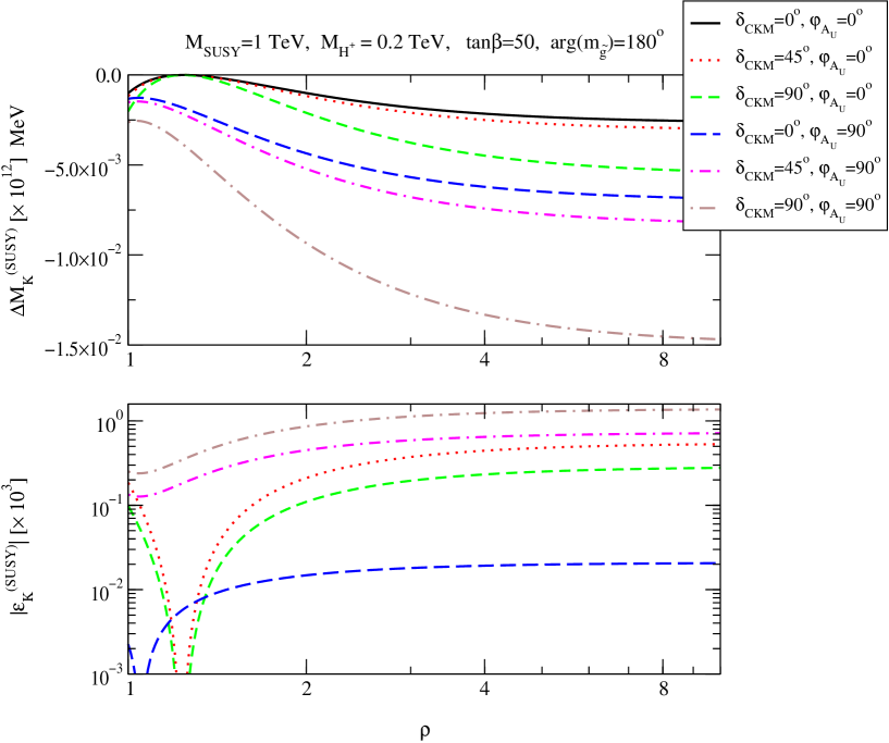
Figure 4: SUSY Higgs-DP contributions to $\epsilon_{K}$ and $\Delta M_{K}$ given in units of $10^{-12}$ MeV and $10^{-3}$, respectively, as functions of the hierarchy factor $\rho$, for $M_{\rm SUSY}=1$ TeV, $M_{H^{+}}=0.2$ TeV, $\tan\beta=50$, and ${\rm arg}\,m_{\tilde{g}}=180^{\circ}$, where the values of $\delta_{\rm CKM}$ and $\phi_{A_{U}}$ are varied discretely.

For the MSSM parameter space under study, there is always a GIM-operative value for the hierarchy factor $\rho$, iff $\phi_{A_{U}}-\phi_{\tilde{g}}=0$ or $\pm\pi$. For $\phi_{A_{U}}-\phi_{\tilde{g}}=0$, we have $\rho_{\rm GIM}<1$, whereas it is $\rho_{\rm GIM}>1$, for $\phi_{A_{U}}-\phi_{\tilde{g}}=\pi$. In fact, the second case is realized in Fig. 4 for $\rho_{\rm GIM}\approx 1.22$, where $\Delta M_{K}^{\rm SUSY}$ and $|\epsilon_{K}^{\rm SUSY}|$ vanish independently of the value of the CKM phase. Here, we should emphasize the fact that the value of $\rho_{\rm GIM}$ does not depend on the FCNC observable under consideration and is in excellent agreement with the one determined by (4.7). Because of the above flavour-universal property of $\rho_{\rm GIM}$, one may even face the very unusual possibility of discovering SUSY at high-energy colliders, without accompanying such a discovery with any new-physics signal in low-energy $K$- and $B$-meson FCNC observables.

It is now instructive to gauge the relative size of the different DP-induced Wilson coefficients in (3.1). For simplicity, let us take $\rho=1$. Then, each individual DP-induced Wilson coefficient in (3.1) may be approximately given by

$$\sum_{i=1}^{3}\,(g^{L}_{H_{i}\bar{s}d})^{2} \approx (\chi_{\rm FC}^{(t)})^{2}\,(V_{ts}^{*}V_{td})^{2}\ \sum_{i=1}^{3}\,\frac{O_{1i}^{2}-O_{3i}^{2}+2\,i\,O_{1i}O_{3i}}{M_{H_{i}}^{2}}\ ,$$

$$\sum_{i=1}^{3}\,(g^{R}_{H_{i}\bar{s}d})^{2} \approx (\chi_{\rm FC}^{(t)*})^{2}\,(V_{ts}^{*}V_{td})^{2}\,\sum_{i=1}^{3}\,\frac{O_{1i}^{2}-O_{3i}^{2}-2\,i\,O_{1i}O_{3i}}{M_{H_{i}}^{2}}\ ,$$

$$\sum_{i=1}^{3}\,(g^{L}_{H_{i}\bar{s}d}\,g^{R}_{H_{i}\bar{s}d}) \approx |\chi_{\rm FC}^{{(t)}}|^{2}\,(V_{ts}^{*}V_{td})^{2}\,\sum_{i=1}^{3}\,\frac{O_{1i}^{2}+O_{3i}^{2}}{M_{H_{i}}^{2}}\ ,$$ (4.8)

where $\chi_{\rm FC}^{{(t)}}$ is the $t$-quark dependent entry of the diagonal matrix $\chi_{\rm FC}$ defined in (2.13). For $M_{H^{+}}\stackrel{{\scriptstyle>}}{{{}_{\sim}}}180$ GeV, CP-violation and Higgs-mixing effects start to decouple from the lightest $H_{1}$-sector [19]. Moreover, in the region $\tan\beta\stackrel{{\scriptstyle>}}{{{}_{\sim}}}40$, the $\Phi_{2}$-component in the $H_{2}$- and $H_{3}$-boson mass-eigenstates is suppressed. As a consequence of the latter, we obtain

$$\sum_{i=1}^{3}\ \frac{O_{1i}^{2}\>-\>O_{3i}^{2}}{M_{H_{i}}^{2}} = \Big{(}\,O^{2}_{11}\>-\>O^{2}_{31}\,\Big{)}\,\Bigg{(}\,\frac{1}{M^{2}_{H_{1}}}\>-\>\frac{1}{M^{2}_{H_{23}}}\,\Bigg{)}\ +\ {\cal O}\Bigg{(}\,\frac{M^{2}_{H_{2}}-M^{2}_{H_{3}}}{M^{2}_{H_{23}}}\,\Bigg{)}\,,$$ (4.9)

$$\sum_{i=1}^{3}\ \frac{O_{1i}\,O_{3i}}{M_{H_{i}}^{2}} = O_{11}\,O_{31}\,\Bigg{(}\,\frac{1}{M^{2}_{H_{1}}}\>-\>\frac{1}{M^{2}_{H_{23}}}\,\Bigg{)}\ +\ {\cal O}\Bigg{(}\,\frac{M^{2}_{H_{2}}-M^{2}_{H_{3}}}{M^{2}_{H_{23}}}\,\Bigg{)}\,,$$ (4.10)

where $M^{2}_{H_{23}}=\frac{1}{2}\,(M^{2}_{H_{2}}+M^{2}_{H_{3}})$ and the orthogonality of the $O$ matrix has been used. Since it is $O_{11},\ O_{31}\ll 1$ in the kinematic region of our interest, then on account of (4.9) and (4.10) and for maximal CKM phase $\delta_{\rm CKM}=90^{\circ}$, the dominant contribution to $\Delta M_{K}^{\rm SUSY}$ and $\epsilon_{K}^{\rm SUSY}$ comes from the last DP expression in (4.1), namely from the Wilson coefficient $C^{\rm LR\,(DP)}_{2}$ in (3.1), despite the additional suppression factor $m_{d}/m_{s}\approx 1/10$ with respect to $C^{\rm SLL\,(DP)}_{1}$. If $\delta_{\rm CKM}=0$, $\Delta M_{K}^{\rm SUSY}$ still receives its largest contribution from $C^{\rm LR\,(DP)}_{2}$, while $|\epsilon_{K}^{\rm SUSY}|$ is dominated by the first DP expression in (4.1), i.e.  from $C^{\rm SLL\,(DP)}_{1}$; the second DP expression in (4.1) is very suppressed with respect to the first one by two powers of the ratio $m_{d}/m_{s}$. From Fig. (3), we also see that in addition to the CKM phase $\delta_{\rm CKM}$, the soft SUSY-breaking CP-phases, such as ${\rm arg}\,(m_{\tilde{g}})$ and ${\rm arg}\,(A_{U})$, may also give rise by themselves to enhancements of $|\Delta M_{K}^{\rm SUSY}|$ and $|\epsilon_{K}^{\rm SUSY}|$ even up to one order of magnitude. Analogous remarks and observations also hold true for the $B$-meson FCNC observables which are to be discussed in the next section.

Finally, we should comment on the fact that the 2HDM contribution by itself due to $C^{\rm LR\,(2HDM)}_{2}$ in (3.9) can only give rise to the undetectably small numerical values, $|\Delta M_{K}^{\rm 2HDM}|=5\times 10^{-17}$ MeV and $|\epsilon_{K}^{\rm 2HDM}|=5\times 10^{-6}$ (indicated by an arrow in the Fig. 3), for $\delta_{\rm CKM}=90^{\circ}$.

4.2 $\Delta M_{B_{q}}$, $B_{q}\to\ell^{+}\ell^{-}$ and associated leptonic CP asymmetries

In this section, we will present numerical estimates for a number of $B$-meson FCNC observables, such as the mass difference $\Delta M_{B_{q}}$, the branching ratio for $B_{q}\to\ell^{+}\ell^{-}$ and the CP asymmetries associated with the $B$-meson leptonic decays. The current experimental status of these observables is as follows [43]:

$$\Delta M_{B_{d}} = 0.489\>\pm\>0.008\ {\rm ps}^{-1}\,,$$ (4.11)

$$\Delta M_{B_{s}} > 13.1\ {\rm ps}^{-1}\,,$$ (4.12)

$${\cal B}(B_{s}\to\mu^{+}\mu^{-}) < 2.0\times 10^{-6}$$ (4.13)

and [46]

$${\cal B}(B_{d}\to\tau^{+}\tau^{-})\ <\ 0.015\,.$$ (4.14)

Future experiments at an upgraded phase of the Tevatron collider may reach higher sensitivity to ${\cal B}(B_{s}\to\mu^{+}\mu^{-})$ up to the $10^{-8}$-level [47, 12, 11].

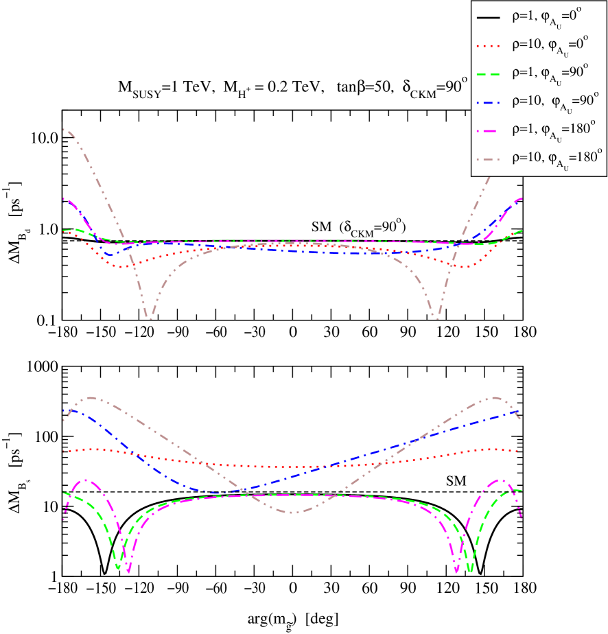
Figure 5: SM and SUSY Higgs-DP contributions to $\Delta M_{B_{d}}$ and $\Delta M_{B_{s}}$ as functions of the gluino phase ${\rm arg}\,(m_{\tilde{g}})$, for $M_{\rm SUSY}=1$ TeV, $M_{H^{+}}=0.2$ TeV, $\tan\beta=50$ and $\delta_{\rm CKM}=90^{\circ}$, where the hierarchy factor $\rho$ and $\phi_{A_{U}}$ are varied independently as shown above. The SM contributions alone for $\delta_{\rm CKM}=90^{\circ}$ are displayed by horizontal dashed lines.

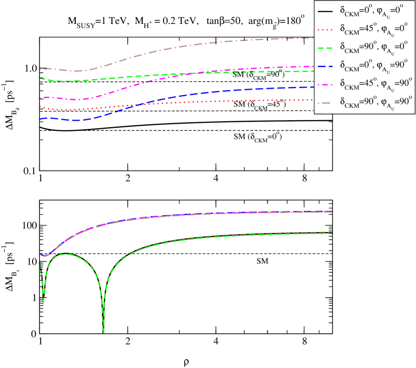
Figure 6: SM and SUSY Higgs-DP contributions to $\Delta M_{B_{d}}$ and $\Delta M_{B_{s}}$ versus the hierarchy factor $\rho$, for $M_{\rm SUSY}=1$ TeV, $M_{H^{+}}=0.2$ TeV, $\tan\beta=50$, and ${\rm arg}\,m_{\tilde{g}}=180^{\circ}$, where $\delta_{\rm CKM}$ and $\phi_{A_{U}}$ obtain discrete values as shown above. Also shown are the SM effects alone for different choices of the CKM phase $\delta_{\rm CKM}$ (horizontal dashed lines).

Let us start our discussion by numerically analyzing the $B$-meson mass differences $\Delta M_{B_{d}}$ and $\Delta M_{B_{s}}$. As in the case of the $K$-meson observables, we use the same input values as those shown in Fig. 2, i.e.  $M_{\rm SUSY}=1$ TeV, $M_{H^{+}}=0.2$ TeV and $\tan\beta=50$. Then, Fig. 5 displays the combined, SM and Higgs-DP, contributions to $\Delta M_{B_{d}}$ and $\Delta M_{B_{s}}$ as functions of the gluino phase ${\rm arg}\,(m_{\tilde{g}})$, for $\delta_{\rm CKM}=90^{\circ}$ and different choices of hierarchy factor $\rho$ and $\phi_{A_{U}}$. Note that the SM contributions alone for $\delta_{\rm CKM}=90^{\circ}$ are displayed by horizontal dashed lines. Even though the SM predictions for $\Delta M_{B_{d,s}}$ may adequately describe by themselves the experimental values in (4.11) and (4.12), they cannot yet decisively exclude possible new-physics contributions due to the inherent uncertainties in the calculation of hadronic matrix elements such as those induced by SUSY Higgs-mediated FCNC interactions. In particular, we observe in Fig. 5 that SM and Higgs-DP effects may add constructively or destructively to the mass differences $\Delta M_{B_{d,s}}$. Similar features are found in Fig. 6, where the SM and SUSY Higgs-DP contributions to $\Delta M_{B_{d}}$ and $\Delta M_{B_{s}}$ are plotted versus the hierarchy factor $\rho$, for discrete values of $\delta_{\rm CKM}$ and $\phi_{A_{U}}$. In our SM CKM-phase convention [43], unlike the CKM matrix element $V_{ts}$, the matrix element $V_{td}$ is very sensitive to $\delta_{\rm CKM}$ values. As a result, the SM predictions for $\Delta M_{B_{d}}$ strongly depend on the selected value of $\delta_{\rm CKM}$, as can be seen from Fig. 6.

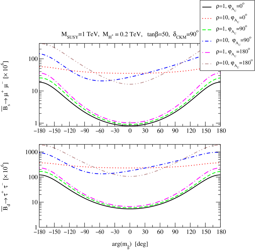
Figure 7: SUSY Higgs-penguin contributions to ${\cal B}(\bar{B}^{0}_{s}\to\mu^{+}\mu^{-})$ and ${\cal B}(\bar{B}^{0}_{d}\to\tau^{+}\tau^{-})$ versus the gluino phase ${\rm arg}\,(m_{\tilde{g}})$, for $M_{\rm SUSY}=1$ TeV, $M_{H^{+}}=0.2$ TeV, $\tan\beta=50$, and $\delta_{\rm CKM}=90^{\circ}$, where $\rho$ and $\phi_{A_{U}}$ are varied discretely.

In Fig. 7, we exhibit numerical values for the branching ratios ${\cal B}(\bar{B}^{0}_{s}\to\mu^{+}\mu^{-})$ and ${\cal B}(\bar{B}^{0}_{d}\to\tau^{+}\tau^{-})$ as functions for the gluino phase ${\rm arg}\,(m_{\tilde{g}})$, for $M_{\rm SUSY}=1$ TeV, $M_{H^{+}}=0.2$ TeV, $\tan\beta=50$, and $\delta_{\rm CKM}=90^{\circ}$, where $\rho$ and $\phi_{A_{U}}$ are varied discretely. Since the branching ratios are driven by Higgs-penguin effects in the region of large $\tan\beta$, predictions for other inputs of $\tan\beta$ and $M_{H^{+}}$ may be easily estimated by rescaling the numerical values by a factor $x_{\cal O}=(\tan\beta/50)^{6}\times(0.2~{}{\rm TeV}/M_{H^{+}})^{4}$, for $\tan\beta\stackrel{{\scriptstyle>}}{{{}_{\sim}}}40$. Thus, confronting the predictions for ${\cal B}(\bar{B}^{0}_{s}\to\mu^{+}\mu^{-})$ with experiment data in (4.13), combined bounds on the $\tan\beta$-$M_{H^{+}}$ plane may be obtained for a given set of soft SUSY-breaking parameters. As we see in Fig. 7, these combined bounds become even more restrictive for large gluino phases, ${\rm arg}\,m_{\tilde{g}}\stackrel{{\scriptstyle>}}{{{}_{\sim}}}90^{\circ}$, in agreement with our discussions in Section 4.1.

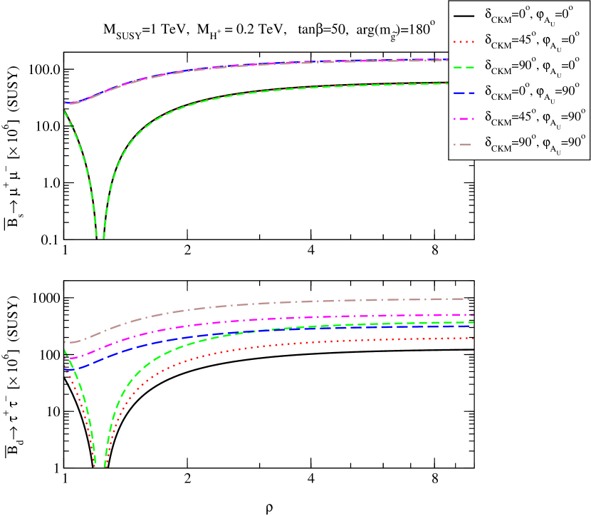
Figure 8: SUSY Higgs-penguin contributions to ${\cal B}(\bar{B}^{0}_{s}\to\mu^{+}\mu^{-})$ and ${\cal B}(\bar{B}^{0}_{d}\to\tau^{+}\tau^{-})$ as functions of the hierarchy factor $\rho$, for $M_{\rm SUSY}=1$ TeV, $M_{H^{+}}=0.2$ TeV, $\tan\beta=50$, and ${\rm arg}\,m_{\tilde{g}}=180^{\circ}$, where $\delta_{\rm CKM}$ and $\phi_{A_{U}}$ take discrete values.

However, there is an additional factor that may crucially affect our predictions for the branching ratios of the decays $\bar{B}^{0}_{s}\to\mu^{+}\mu^{-}$ and $\bar{B}^{0}_{d}\to\tau^{+}\tau^{-}$, namely the hierarchy parameter $\rho$. As we show in Fig. 8, even for the extreme choice of a gluino phase ${\rm arg}\,m_{\tilde{g}}=180^{\circ}$, ${\cal B}(\bar{B}^{0}_{d}\to\mu^{+}\mu^{-})$ and ${\cal B}(\bar{B}^{0}_{s}\to\mu^{+}\mu^{-})$ can get very suppressed for a specific value of $\rho$ in certain soft SUSY-breaking scenarios that can realize a GIM-operative point in their parameter space. As we detailed in Section 4.1, this phenomenon occurs for the universal value of $\rho=\rho_{\rm GIM}=1.22$, when $\phi_{A_{U}}-\phi_{\tilde{g}}=\pm 180^{\circ}$. As can be seen in Fig. 8, the predicted values for $\bar{B}^{0}_{s}\to\mu^{+}\mu^{-}$ and $\bar{B}^{0}_{d}\to\tau^{+}\tau^{-}$, where $\phi_{A_{U}}=0^{\circ}$, confirm the above observation.

As we have already mentioned, the observables $\Delta M_{B_{s}}$ and ${\cal B}(\bar{B}_{s}^{0}\to\mu^{+}\mu^{-})$ exhibit a different scaling behaviour with respect to $M_{H^{+}}$ and $\tan\beta$, through the scaling factor $x_{\cal O}$ in (4.1). Once the above two kinematic parameters are fixed to some input values, the two observables $\Delta M_{B_{s}}$ and ${\cal B}(\bar{B}_{s}^{0}\to\mu^{+}\mu^{-})$ are then rather correlated to each other, since their dependences on the $\mu$-parameter and $A_{U}$ are very similar in the minimal flavour-violating case $\rho=1$ [14]. As one can see from Figs. 5–8, our numerical analysis agrees well with the above result for $\rho=1$. However, we also observe that the correlation is practically lost for $\rho>1$, e.g. close to the GIM-operative points, and/or by the inclusion of CP-violating effects, as $\Delta M_{B_{s}}$ and ${\cal B}(\bar{B}_{s}^{0}\to\mu^{+}\mu^{-})$ have different dependences on the soft CP-odd phases.

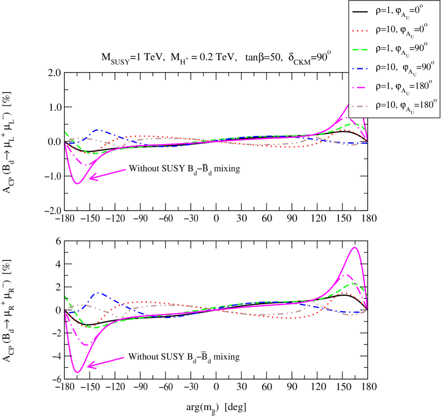
Figure 9: Numerical values for the CP asymmetries ${\cal A}_{\rm CP}^{(B^{0}_{d}\to\mu^{+}_{L}\mu^{-}_{L})}$ and ${\cal A}_{\rm CP}^{(B^{0}_{d}\to\mu^{+}_{R}\mu^{-}_{R})}$ as functions of the gluino phase ${\rm arg}\,(m_{\tilde{g}})$, for $M_{\rm SUSY}=1$ TeV, $M_{H^{+}}=0.2$ TeV, $\tan\beta=50$, and $\delta_{\rm CKM}=90^{\circ}$, where $\rho$ and $\phi_{A_{U}}$ are varied discretely. Also shown is the prediction for the CP asymmetries without including $B^{0}_{d}$-$\bar{B}^{0}_{d}$ mixing.

Let us now investigate the size of the CP asymmetries in the leptonic $B_{d}$-meson decays in the CP-violating MSSM; the corresponding CP asymmetries for the $B_{s}$ meson are experimentally constrained to be rather small, less than 5% (see also discussion after (3.32)). In Fig. 9, we display numerical values for the CP asymmetries ${\cal A}_{\rm CP}^{(B^{0}_{d}\to\mu^{+}_{L}\mu^{-}_{L})}$ and ${\cal A}_{\rm CP}^{(B^{0}_{d}\to\mu^{+}_{R}\mu^{-}_{R})}$ as functions of the gluino phase ${\rm arg}\,(m_{\tilde{g}})$, for $M_{\rm SUSY}=1$ TeV, $M_{H^{+}}=0.2$ TeV, $\tan\beta=50$, and $\delta_{\rm CKM}=90^{\circ}$. As usual, we independently vary the parameters $\rho$ and $\phi_{A_{U}}$ to take on the discrete values $\rho=1,\ 10$ and $\phi_{A_{U}}=0^{\circ},90^{\circ}$ and $180^{\circ}$. We find that if the $B^{0}_{d}$-$\bar{B}^{0}_{d}$ mixing is consistently taken into account, the typical size of ${\cal A}_{\rm CP}^{(B^{0}_{d}\to\mu^{+}_{L}\mu^{-}_{L})}$ and ${\cal A}_{\rm CP}^{(B^{0}_{d}\to\mu^{+}_{R}\mu^{-}_{R})}$ does not exceed 0.7% and 3%, respectively. If $B^{0}_{d}$-$\bar{B}^{0}_{d}$ mixing is not included, the CP asymmetries can reach slightly higher values up to 1.2% and 6%, respectively. The apparent reason for the smallness of the CP asymmetries is due to the occurrence of an approximate cancellation in the sum $C_{S}+C_{P}$ in (3.32) at large $\tan\beta$, as the muon velocity is $\beta_{\mu}\approx 1$.

Having gained some insight from the above exercise, one may seek alternative ways to enhance the di-muon asymmetries ${\cal A}_{\rm CP}^{(B_{d}^{0}\to\mu_{L,(R)}^{+}\mu_{L,(R)}^{-})}$. To this end, the first attempt would be to suppress the effect of the $B_{d}^{0}-\bar{B}_{d}^{0}$ mixing by considering smaller $\tan\beta$ values, e.g.  $\tan\beta\stackrel{{\scriptstyle<}}{{{}_{\sim}}}10$. In this intermediate region of $\tan\beta$, the above cancellation in the sum $C_{S}+C_{P}$ does not occur due to non-trivial CP-violating Higgs-mixing effects and so the CP asymmetries ${\cal A}_{\rm CP}^{(B_{d}^{0}\to\mu_{L,(R)}^{+}\mu_{L,(R)}^{-})}$ can be significantly increased. To get an idea of the magnitude of the CP asymmetries in this case, we consider the so-called CPX scenario introduced in [48] to maximize CP-violating effects in the lightest Higgs sector of an effective MSSM. In the CPX scenario, the $\mu$-parameter and the soft trilinear Yukawa coupling $A_{U}$ are set by the relations: $\mu=4M_{\rm SUSY}$ and $A_{U}=2M_{\rm SUSY}$. Thus, for $M_{H^{+}}=0.15$ TeV, $M_{\rm SUSY}=1$ TeV, $\tan\beta=7$, $\rho=10$, $\phi_{A_{U}}=45^{\circ}$ and $\phi_{\tilde{g}}=0^{\circ}$, we find that CP-violating Higgs-penguin effects can give rise to the CP asymmetries:

$${\cal A}_{\rm CP}^{(B_{d}^{0}\to\mu_{L}^{+}\mu_{L}^{-})}\ \approx\ -9~{}\%\,,\qquad{\cal A}_{\rm CP}^{(B_{d}^{0}\to\mu_{R}^{+}\mu_{R}^{-})}\ \approx\ -37~{}\%$$ (4.15)

where ${\cal B}(B_{d}\to\mu^{+}\mu^{-})=3.6\times 10^{-10}$, which is an order of magnitude larger than the SM prediction [41]. Another variant of the CPX scenario of equally phenomenological importance utilizes the parameters: $\tan\beta=10$, $\rho=10$, $\phi_{A_{U}}=45^{\circ}$ and $\phi_{\tilde{g}}=90^{\circ}$, with $M_{\rm SUSY}=1$ TeV. In this case, we obtain

$${\cal A}_{\rm CP}^{(B_{d}^{0}\to\mu_{L}^{+}\mu_{L}^{-})}\ \approx\ 11~{}\%\,,\qquad{\cal A}_{\rm CP}^{(B_{d}^{0}\to\mu_{R}^{+}\mu_{R}^{-})}\ \approx\ 43~{}\%$$ (4.16)

and ${\cal B}(B_{d}\to\mu^{+}\mu^{-})=4.1\times 10^{-9}$, which is two orders of magnitude above the SM prediction. The above scenario appears to pass all the experimental constraints, including those deduced from LEP2 analyses of direct Higgs searches [48, 49]. Most interestingly, a possible observation of a non-zero CP asymmetry in the leptonic di-muon channel will constitute the harbinger for new physics at $B$ factories. At this stage, it is important to comment on the fact that the numerical values stated in (4.15) and (4.16) should be viewed as crude estimates, since they are obtained entirely on the basis of our resummed FCNC effective Lagrangian (2.18) at the intermediate $\tan\beta$ regime. However, in this region of $\tan\beta$, we expect additional one-loop effects to start getting relevant, such as supersymmetric $Z$-penguin and box diagrams. Even though our initial estimates given above appear to yield rather encouraging results, a complete study of the leptonic $B$-meson branching ratios and the respective CP asymmetries for all values of $\tan\beta$ would be preferable.

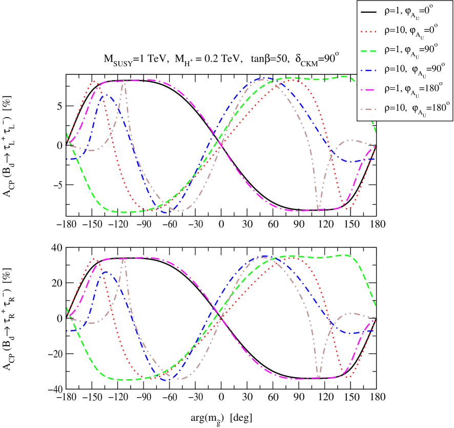
Figure 10: Numerical estimates of the CP asymmetries ${\cal A}_{\rm CP}^{(B^{0}_{d}\to\tau^{+}_{L}\tau^{-}_{L})}$ and ${\cal A}_{\rm CP}^{(B^{0}_{d}\to\tau^{+}_{R}\tau^{-}_{R})}$ versus the gluino phase ${\rm arg}\,(m_{\tilde{g}})$, for $M_{\rm SUSY}=1$ TeV, $M_{H^{+}}=0.2$ TeV, $\tan\beta=50$, and $\delta_{\rm CKM}=90^{\circ}$, where $\rho$ and $\phi_{A_{U}}$ take discrete values as shown above.

In the case of $\tau$-lepton CP asymmetries, the velocities of the decayed $\tau$-leptons $\beta_{\tau}$ is roughly 0.5, so one naturally gets an appreciably higher value for the expression $\beta_{\tau}\,C_{S}+C_{P}\approx 0.5C_{P}$ in (3.32). As a result, larger values for the $\tau$-lepton CP asymmetries are expected. Indeed, in Fig. 10, we display numerical predictions for ${\cal A}_{\rm CP}^{(B^{0}_{d}\to\tau^{+}_{L}\tau^{-}_{L})}$ and ${\cal A}_{\rm CP}^{(B^{0}_{d}\to\tau^{+}_{R}\tau^{-}_{R})}$ versus the gluino phase ${\rm arg}\,(m_{\tilde{g}})$, for the same values of the input parameters as in Fig. 9. Then, the CP asymmetries ${\cal A}_{\rm CP}^{(B^{0}_{d}\to\tau^{+}_{L}\tau^{-}_{L})}$ and ${\cal A}_{\rm CP}^{(B^{0}_{d}\to\tau^{+}_{R}\tau^{-}_{R})}$ can be as high as 9% and 36%, respectively.

We conclude this section with some general remarks. In addition to the $K$- and $B$-meson observables we have been studying here, there is a large number of other FCNC observables which have to be considered in a combined full-fledged analysis. For example, the decay $B\to X_{s}\gamma$ [50, 51] plays a central rôle in such a global analysis, because it will enable us to delineate more accurately the CP-conserving/CP-violating soft SUSY-breaking parameter space favoured by low-energy FCNC observables. In this context, constraints on CP-violating SUSY phases from the non-observation of electron and neutron electric dipole moments (EDMs) should also be implemented. Large CP gluino and stop phases, as the ones considered in our analysis, would require either very heavy squarks with masses larger than 5-6 TeV or the existence of a cancellation mechanism among the different one-, two- and higher-loop EDM contributions [52, 53, 23]. Especially, it has been shown recently [23] that if the first two generation of squarks are heavier than about 3 TeV, the required degree of cancellations does not exceed the 10% level and hence large CP-violating gluino, gaugino and third-generation phases are still allowed for wide regions of the MSSM parameter space. Finally, in the present numerical analysis, we have concentrated on scenarios that minimally depart from the minimal flavour-violation assumption through the presence of diagonal, but non-universal squark masses. In the most general case, however, the squark mass matrices and consequently the resummation matrix ${\bf{R}}$ of the radiative threshold effects may not be diagonal. Such low-energy realizations with off-diagonal soft squark-mass matrices can still be treated exactly within the context of our resummed FCNC effective Lagrangian (2.18), by appropriately considering non-trivial quark-squark CKM-like matrices, such as the 3-by-3 unitary matrix ${\bf{\cal U}_{L}^{Q}}$ in (2.9).

5 Conclusions

We have derived the general form for the effective Lagrangian of Higgs-mediated FCNC interactions to $d$-type quarks, where large-$\tan\beta$ radiative threshold effects have been resummed consistently (cf. (2.18) and (2)). Our resummed FCNC effective Lagrangian is free from pathological singularities, which mainly emanate from the top-quark dominance hypothesis frequently adopted in the literature, and has been appropriately generalized to include effects of non-universality in the squark sector, as well as CP-violation effects originating from the CKM-mixing matrix and the complex soft SUSY-breaking masses. In particular, our resummed effective Lagrangian can be applied to study Higgs-mediated FCNC effects in more general soft SUSY-breaking scenarios, beyond those that have already been discussed within the restricted framework of models with minimal flavour violation. Also, an approach to resumming radiative threshold effects, very analogous to the one developed in Section 2, can straightforwardly be applied to see-saw SUSY models, so as to properly describe Higgs-mediated lepton-flavour-violating interactions.

Within the context of generic soft SUSY-breaking scenarios, we have analyzed a number of $K$- and $B$-meson observables, such as $\Delta M_{K,B}$, $\epsilon_{K}$, $\epsilon^{\prime}/\epsilon$, ${\cal B}(B_{s,d}\to\ell^{+}\ell^{-})$ and their associated leptonic asymmetries [54], which are enhanced by Higgs-boson FCNC interactions for large values of $\tan\beta$. We have found that the predictions crucially depend on the choice of soft CP-violating phases in a given set of soft SUSY-breaking parameters. For example, for certain values of the gluino and stop phases, the predictions can reach and even exceed the current experimental limits, whereas for other values of the CP-odd phases the FCNC effects can be reduced by one or even two orders of magnitude. Most remarkably, we have been able to identify configurations in the soft SUSY-breaking parameter space, such as $\rho_{\rm GIM}$, where a kind of a GIM-cancellation mechanism becomes fully operative [cf. (4.7)] and, as a result of the latter, all Higgs-mediated, $\tan\beta$-enhanced effects on $K$- and $B$-meson FCNC observables are completely absent.

Based on our resummed effective Lagrangian, one may now carry over the present analysis to a vast number of other $K$- and $B$-meson observables. Evidently, further dedicated studies need be performed in this direction. We expect the obtained predictions to affect other low- and high-energy observables, such as measurements of electron and neutron electric dipole moments and Higgs-boson searches, as well as studies on cosmological electroweak baryogenesis and dark matter. It would be very interesting to determine to which degree the emerging CP-violating MSSM framework with CP-mixed Higgs bosons mediating $\tan\beta$-enhanced interactions to matter could be potentially responsible for all the present and future CP-conserving/CP-violating FCNC effects observed in nature.

Acknowledgements

We wish to thank Ulrich Nierste and Alexander Kagan for illuminating discussions, and Herbi Dreiner for a critical reading of the manuscript. A.D. acknowledges financial support from the CERN Theory Division and the Network RTN European Program HPRN-CT-2000-00148 “Physics Across the Present Energy Frontier: Probing the Origin of Mass.” A.P. thanks the Fermilab Theory Group for warm hospitality and support.

Figure 2: Schematic representation of the SUSY mass spectrum considered in our numerical analysis, where $m_{\tilde{q}}$ and $m_{\tilde{t}}$ denote the masses of the first two and third generations of squarks, respectively. The hierarchy factor $\rho$, the phase $\phi_{\tilde{g}}$ of the gluino mass, and the phases $\phi_{A_{t,b}}$ of the soft SUSY breaking trilinear couplings, with $\phi_{A_{t}}=\phi_{A_{b}}=\phi_{A_{U}}$, are varied independently (see also discussion in the text).

References

- [1] S.L. Glashow and S. Weinberg, Phys. Rev. D15 (1977) 1958.
- [2] T.P. Cheng and M. Sher, Phys. Rev. D35 (1987) 3484; G.C. Branco, A.J. Buras and J.M. Gerard, Nucl. Phys. B259 (1985) 306.
- [3] T. Banks, Nucl. Phys. B303 (1988) 172; E. Ma, Phys. Rev. D39 (1989) 1922.
- [4] R. Hempfling, Phys. Rev. D49 (1994) 6168; L.J. Hall, R. Rattazzi and U. Sarid, Phys. Rev. D50 (1994) 7048; T. Blazek, S. Raby and S. Pokorski, Phys. Rev. D52 (1995) 4151; M. Carena, M. Olechowski, S. Pokorski and C.E.M. Wagner, Nucl. Phys. B426 (1994) 269; S. Heinemeyer, W. Hollik and G. Weiglein, Phys. Lett. B440 (1998) 296; Eur. Phys. J. C9 (1999) 343; F. Borzumati, G. Farrar, N. Polonsky and S. Thomas, Nucl. Phys. B555 (1999) 53; J.R. Espinosa and R.J. Zhang, Nucl. Phys. B586 (2000) 3.
- [5] C.S. Huang and Q.-S. Yan, Phys. Lett. B442 (1998) 209; S.R. Choudhury and N. Gaur, Phys. Lett. B451 (1999) 86; C.S. Huang, W. Liao and Q.-S. Yuan, Phys. Rev. D59 (1999) 011701; C. Hamzaoui, M. Pospelov and M. Toharia, Phys. Rev. D59 (1999) 095005.
- [6] K.S. Babu and C. Kolda, Phys. Rev. Lett. 84 (2000) 228.
- [7] M. Carena, D. Garcia, U. Nierste and C.E. Wagner, Nucl. Phys. B577 (2000) 88.
- [8] P.H. Chankowski and Lucja Slawianowska, Phys. Rev. D63 (2001) 054012; C.S. Huang, W. Liao, Q.-S. Yuan and S.-H. Zhu, Phys. Rev. D63 (2001) 114021.
- [9] C. Bobeth, T. Ewerth, F. Krüger and J. Urban, Phys. Rev. D64 (2001) 074014.
- [10] G. Isidori and A. Retico, JHEP 0111 (2001) 001; hep-ph/0208159.
- [11] A. Dedes, H.K. Dreiner and U. Nierste, Phys. Rev. Lett. 87 (2001) 251804; A. Dedes, H.K. Dreiner, U. Nierste and P. Richardson, hep-ph/0207026.
- [12] R. Arnowitt, B. Dutta, T. Kamon and M. Tanaka, Phys. Lett. B538 (2002) 121; S. Baek, P. Ko and W.Y. Song, hep-ph/0208112.
- [13] G. D’Ambrosio, G.F. Giudice, G. Isidori and A. Strumia, hep-ph/0207036.
- [14] A.J. Buras, P.H. Chankowski, J. Rosiek and L. Slawianowska, hep-ph/0207241.
- [15] J.K. Mizukoshi, X. Tata and Y. Wang, hep-ph/0208078.
- [16] T. Ibrahim and P. Nath, hep-ph/0208142.
- [17] N. Cabibbo, Phys. Rev. Lett. 10 (1963) 531; M. Kobayashi and T. Maskawa, Prog. Theor. Phys. 49 (1973) 652.
- [18] S.L. Glashow, J. Iliopoulos and L. Maiani, Phys. Rev. D2 (1970) 1285.
- [19] M. Carena, J. Ellis, A. Pilaftsis and C.E.M. Wagner, Nucl. Phys. B586 (2000) 92.
- [20] For example, gaugino-Higgsino mixing effects studied in [15] and [16] can be straightforwardly included in our formalism.
- [21] A. Pilaftsis, Phys. Rev. D58 (1998) 096010; Phys. Lett. B435 (1998) 88.
- [22] A. Pilaftsis and C.E.M. Wagner, Nucl. Phys. B553 (1999) 3; D.A. Demir, Phys. Rev. D60 (1999) 055006; S.Y. Choi, M. Drees and J.S. Lee, Phys. Lett. B481 (2000) 57; G.L. Kane and L.-T. Wang, Phys. Lett. B488 (2000) 383; T. Ibrahim and P. Nath, Phys. Rev. D63 (2001) 035009; hep-ph/0204092; S.Y. Choi, K. Hagiwara and J.S. Lee, Phys. Rev. D64 (2001) 032004; S. Heinemeyer, Eur. Phys. J. C22 (2001) 521; M. Carena, J. Ellis, A. Pilaftsis and C.E.M. Wagner, Nucl. Phys. B625 (2002) 345; M. Boz, Mod. Phys. Lett. A17 (2002) 215; S.W. Ham, S.K. Oh, E.J. Yoo, C.M. Kim and D. Son, hep-ph/0205244.
- [23] A. Pilaftsis, Nucl. Phys. B644 (2002) 263.
- [24] From a Feynman–diagrammatic point of view, resummation of radiative threshold corrections is equivalent to resumming wave-function graphs in the on-shell renormalization scheme. For a detailed discussion on this issue, see H.E. Logan and U. Nierste, Nucl. Phys. B586 (2000) 39 and [7].
- [25] For reviews on kaon physics, see, E.A. Paschos and U. Türke, Phys. Rept. 178 (1989) 145; W. Grimus, Fortschr. Phys. 36 (1988) 201; R. Decker, Fortschr. Phys. 37 (1989) 657; L. Lavoura, Annals Phys. 207 (1991) 428; B. Weinstein and L. Wolfenstein, Rev. Mod. Phys. 65 (1993) 1113.
- [26] For pedagogical introductions to CP violation in the -meson system, see, M. Neubert, Int. J. Mod. Phys. A11 (1996) 4173; A.J. Buras, hep-ph/9806471.
- [27] G.C. Branco, L. Lavoura and J.P. Silva, Oxford, UK: Clarendon (1999), p. 511.
- [28] A.J. Buras, S. Jäger and J. Urban, Nucl. Phys. B605 (2001) 600.
- [29] A.J. Buras, P.H. Chankowski, J. Rosiek and L. Slawianowska, Nucl. Phys. B619 (2001) 434.
- [30] M. Ciuchini et al., JHEP 0107 (2001) 013.
- [31] A.J. Buras, M. Misiak and J. Urban, Nucl. Phys. B586 (2000) 397.
- [32] D. Becirevic, V. Gimenez, G. Martinelli, M. Papinutto and J. Reyes, Nucl. Phys. Proc. Suppl. 106 (2002) 385.
- [33] G. Buchalla, A.J. Buras and M.K. Harlander, Nucl. Phys. B337 (1990) 313.
- [34] T. Hambye, G.O. Kohler, E.A. Paschos, P.H. Soldan and W.A. Bardeen, Phys. Rev. D58 (1998) 014017; T. Hambye, G.O. Kohler, E.A. Paschos and P.H. Soldan, Nucl. Phys. B564 (2000) 391.
- [35] S. Bosch, A.J. Buras, M. Gorbahn, S. Jäger, M. Jamin, M.E. Lautenbacher and L. Silvestrini, Nucl. Phys. B565 (2000) 3.
- [36] E. Gabrielli and G.F. Giudice, Nucl. Phys. B433 (1995) 3.
- [37] G. Colangelo and G. Isidori, JHEP 9809 (1998) 009; A.J. Buras, G. Colangelo, G. Isidori, A. Romanino and L. Silvestrini, Nucl. Phys. B566 (2000) 3.
- [38] A.L. Kagan and M. Neubert, Phys. Rev. Lett. 83 (1999) 4929; A.J. Buras, P. Gambino, M. Gorbahn, S. Jäger and L. Silvestrini, Nucl. Phys. B592 (2001) 55; C.H. Chen, Phys. Lett. B541 (2002) 155.
- [39] Y. Nir, hep-ph/0208080.
- [40] A. Dedes, J. Ellis and M. Raidal, hep-ph/0209207.
- [41] See second reference in [11].
- [42] C.S. Huang and W. Liao, Phys. Lett. B525 (2002) 107; Phys. Lett. B538 (2002) 301; P.H. Chankowski and L. Slawianowska, Acta Phys. Polon. B32 (2001) 1895.
- [43] K. Hagiwara et al. [Particle Data Group Collaboration], Phys. Rev. D66 (2002) 010001.
- [44] For instance, see, S. Herrlich and U. Nierste, Phys. Rev. D52 (1995) 6505.
- [45] See, for example, J.F. Donoghue, H.P. Nilles and D. Wyler, Phys. Lett. B128 (1983) 55; J.M. Gerard, W. Grimus, A. Raychaudhuri and G. Zoupanos, Phys. Lett. B140 (1984) 349.
- [46] Y. Grossman, Z. Ligeti and E. Nardi, Phys. Rev. D55 (1997) 2768.
- [47] K. Anikeev et al., hep-ph/0201071.
- [48] M. Carena, J. Ellis, A. Pilaftsis and C.E.M. Wagner, Phys. Lett. B495 (2000) 155.
- [49] For a recent review on Higgs phenomenology, see M. Carena and H.E. Haber, hep-ph/0208209.
- [50] S. Bertolini, F. Borzumati, A. Masiero and G. Ridolfi, Nucl. Phys. B353 (1991) 591; F.M. Borzumati, Z. Phys. C63 (1994) 291.
- [51] G. Degrassi, P. Gambino and G.F. Giudice, JHEP 0012 (2000) 009; M. Carena, D. Garcia, U. Nierste and C. E. Wagner, Phys. Lett. B499 (2001) 141; D.A. Demir and K.A. Olive, Phys. Rev. D65 (2002) 034007.
- [52] T. Ibrahim and P. Nath, Phys. Rev. D58 (1998) 111301; Phys. Rev. D61 (2000) 093004; M. Brhlik, G.J. Good and G.L. Kane, Phys. Rev. D59 (1999) 115004; S. Pokorski, J. Rosiek and C.A. Savoy, Nucl. Phys. B570 (2000) 81; E. Accomando, R. Arnowitt and B. Dutta, Phys. Rev. D61 (2000) 115003; A. Bartl, T. Gajdosik, W. Porod, P. Stockinger and H. Stremnitzer, Phys. Rev. D60 (1999) 073003; T. Falk, K.A. Olive, M. Pospelov and R. Roiban, Nucl. Phys. B60 (1999) 3.
- [53] D. Chang, W.-Y. Keung and A. Pilaftsis, Phys. Rev. Lett. 82 (1999) 900; S.A. Abel, S. Khalil and O. Lebedev, Nucl. Phys. B606 (2001) 151.
- [54] Our numerical analysis has been performed with the Fortran code FCNC.f, which can be accessed from the web site: http://pilaftsi.home.cern.ch/pilaftsi/.