Abstract

The leading electroweak MSSM two-loop corrections to the electroweak precision observables are calculated. They are obtained by evaluating the two-loop ${\cal O}(\alpha_{t}^{2})$, ${\cal O}(\alpha_{t}\alpha_{b})$, ${\cal O}(\alpha_{b}^{2})$ contributions to the quantity $\Delta\rho$ in the limit of heavy scalar quarks, i.e. we consider the contributions of a Two-Higgs-Doublet model with MSSM restrictions. The full analytic result for arbitrary values of the lightest ${\cal CP}$-even Higgs boson mass is presented. The numerical effects of the leading electroweak MSSM two-loop corrections on the precision observables $M_{W}$ and $\sin^{2}\theta_{\mathrm{eff}}$ are analyzed. The electroweak two-loop contribution to $M_{W}$ amounts up to $-12\,\,\mathrm{MeV}$ and up to $+6\times 10^{-5}$ for $\sin^{2}\theta_{\mathrm{eff}}$. The corrections from the bottom quark loops can become important for large values of $\tan\beta$. They enter with a different sign than the ${\cal O}(\alpha_{t}^{2})$ corrections. We furthermore investigate the current sensitivity of the electroweak precision observables to the top Yukawa coupling in the SM and the MSSM. The prospects for indirectly determining this coupling at the next generation of colliders are discussed.

1 Introduction

Theories based on Supersymmetry (SUSY) [1] are widely considered as the theoretically most appealing extension of the Standard Model (SM). They are consistent with the approximate unification of the gauge coupling constants at the GUT scale and provide a way to cancel the quadratic divergences in the Higgs sector hence stabilizing the huge hierarchy between the GUT and the Fermi scales. Furthermore, in SUSY theories the breaking of the electroweak symmetry is naturally induced at the Fermi scale, and the lightest supersymmetric particle can be neutral, weakly interacting and absolutely stable, providing therefore a natural solution for the Dark Matter problem.

Supersymmetry predicts the existence of scalar partners $\tilde{f}_{L},\tilde{f}_{R}$ to each SM chiral fermion, and spin–1/2 partners to the gauge bosons and to the scalar Higgs bosons. So far, the direct search for SUSY particles has not been successful. One can only set lower bounds of ${\cal O}(100)$ GeV on their masses [2]. Furthermore, contrary to the SM two Higgs doublets are required resulting in five physical Higgs bosons [3]. The direct search resulted in lower limits of about $90\,\,\mathrm{GeV}$ for the neutral Higgs bosons and about $80\,\,\mathrm{GeV}$ for the charged ones [4].

An alternative way to probe SUSY is via the virtual effects of the additional particles to precision observables. This requires a very high precision of the experimental results as well as of the theoretical predictions. The most prominent role in this respect plays the $\rho$-parameter [5]. The radiative corrections from vector boson self-energies to the quantity $\Delta\rho$ constitute the leading, process independent corrections to many electroweak precision observables, such as the prediction for $\Delta r$, i.e. the $M_{W}-M_{Z}$ interdependence, and the effective leptonic weak mixing angle, $\sin^{2}\theta_{\mathrm{eff}}$.

The radiative corrections to the electroweak precision observables within the Minimal Supersymmetric Standard Model (MSSM) stemming from scalar fermions, charginos, neutralinos and Higgs bosons have been discussed at the one-loop level in Refs. [6, 7], providing the full one-loop corrections. More recently also the leading two-loop corrections in ${\cal O}(\alpha\alpha_{s})$ to the quark and scalar quark loops for $\Delta\rho$ have been obtained [8] as well as the gluonic two-loop corrections to the $M_{W}-M_{Z}$ interdependence [9]. Contrary to the SM case, these two-loop corrections turned out to increase the one-loop contributions, leading to an enhancement of up to 35% [8].

In this paper we present the leading two-loop corrections to $\Delta\rho$ at ${\cal O}(\alpha_{t}^{2})$, ${\cal O}(\alpha_{t}\alpha_{b})$, ${\cal O}(\alpha_{b}^{2})$, i.e. the leading two-loop contributions involving the top and bottom Yukawa couplings. These contributions are of particular interest, since they involve corrections proportional to $m_{t}^{4}$ and bottom loop corrections enhanced by $\tan\beta$, the ratio of the two vacuum expectation values. For a large SUSY scale, $M_{\rm SUSY}\gg M_{Z}$, the contributions from loops of SUSY particles decouple from physical observables [10, 8]. Therefore, focusing on the case of large $M_{\rm SUSY}$, we derive the leading electroweak two-loop corrections in the limit where besides the SM particles only the two Higgs doublets of the MSSM are active.

As a first step, in Ref. [11] we have calculated the ${\cal O}(\alpha_{t}^{2})$ corrections in the limit where the lightest ${\cal CP}$-even Higgs boson mass vanishes, i.e. $m_{h}\to 0$. The numerical effect of these corrections turned out to be relatively small. However, for the corresponding SM result it was found that the $M_{H}^{\mathrm{SM}}=0$ limit is only a poor approximation of the result with arbitrary $M_{H}^{\mathrm{SM}}$ [12]. Since a similar behavior can be expected for the MSSM, we perform the calculation of the leading electroweak two-loop corrections, ${\cal O}(\alpha_{t}^{2})$, ${\cal O}(\alpha_{t}\alpha_{b})$, and ${\cal O}(\alpha_{b}^{2})$, for arbitrary values of $m_{h}$. The result obtained in the MSSM is compared with the corresponding SM correction of ${\cal O}(\alpha_{t}^{2})$ [12]. The resulting shift in $M_{W}$ and $\sin^{2}\theta_{\mathrm{eff}}$ is analyzed numerically.

Since the top Yukawa coupling enters the predictions for the electroweak precision observables at lowest order in the perturbative expansion at ${\cal O}(\alpha_{t}^{2})$, these contributions allow to study the sensitivity of the precision observables on this coupling. Using a simple approach in which we treat the top Yukawa coupling in the SM and the MSSM as a free parameter, we study the current sensitivities of the electroweak precision observables as well as the prospective accuracies at the next generation of colliders.

The rest of the paper is organized as follows: in Sect. 2 we review the SM and MSSM corrections to the quantity $\Delta\rho$ and present the details of the calculation of the ${\cal O}(\alpha_{t}^{2})$, ${\cal O}(\alpha_{t}\alpha_{b})$, ${\cal O}(\alpha_{b}^{2})$ corrections. Explicit formulas for the results of ${\cal O}(\alpha_{t}^{2})$, ${\cal O}(\alpha_{t}\alpha_{b})$, and ${\cal O}(\alpha_{b}^{2})$ can be found in Sect. 3 and the appendix. The numerical analysis is performed in Sect. 4. In Sect. 5 we analyze the sensitivity of the electroweak precision observables to the top Yukawa coupling. We conclude with Sect. 6.

2 Calculation of the ${\cal O}(\alpha_{t}^{2})$, ${\cal O}(\alpha_{t}\alpha_{b})$, and ${\cal O}(\alpha_{b}^{2})$
corrections

2.1 One-loop results

The quantity $\Delta\rho$,

$$\Delta\rho=\frac{\Sigma_{Z}(0)}{M_{Z}^{2}}-\frac{\Sigma_{W}(0)}{M_{W}^{2}},$$ (1)

parameterizes the leading universal corrections to the electroweak precision observables induced by the mass splitting between fields in an isospin doublet [5]. $\Sigma_{Z,W}(0)$ denote the transverse parts of the unrenormalized $Z$ and $W$ boson self-energies at zero momentum transfer, respectively. $\Delta\rho$ gives the dominant contribution to electroweak precision observables, such as the $W$ boson mass, $M_{W}$, and the effective leptonic mixing angle, $\sin^{2}\theta_{\mathrm{eff}}$. The induced shifts are in leading order given by (with $1-s_{W}^{2}=c_{W}^{2}=M_{W}^{2}/M_{Z}^{2}$)

$$\delta M_{W}\approx\frac{M_{W}}{2}\frac{c_{W}^{2}}{c_{W}^{2}-s_{W}^{2}}\Delta\rho,\quad\delta\sin^{2}\theta_{\mathrm{eff}}\approx-\frac{c_{W}^{2}s_{W}^{2}}{c_{W}^{2}-s_{W}^{2}}\Delta\rho.$$ (2)

In the SM the dominant contribution to $\Delta\rho$ at the one-loop level is given by the $t/b$ doublet due to their large mass splitting. It reads

$$\Delta\rho^{\mathrm{SM}}_{0}=\frac{3\,G_{F}}{8\,\sqrt{2}\,\pi^{2}}\;F_{0}(m_{t}^{2},m_{b}^{2}),$$ (3)

with

$$F_{0}(x,y)=x+y-\frac{2\,x\,y}{x-y}\log\frac{x}{y}.$$ (4)

$F_{0}$ has the properties $F_{0}(m_{a}^{2},m_{b}^{2})=F_{0}(m_{b}^{2},m_{a}^{2})$, $F_{0}(m^{2},m^{2})=0$, $F_{0}(m^{2},0)=m^{2}$. Therefore for $m_{t}\gg m_{b}$ eq. (3) reduces to the well known quadratic correction in $m_{t}$,

$$\Delta\rho^{\mathrm{SM}}_{0}=\frac{3\,G_{F}}{8\,\sqrt{2}\,\pi^{2}}\;m_{t}^{2}.$$ (5)

Within the MSSM the dominant correction from SUSY particles at the one-loop level arises from the scalar top and bottom contribution to eq. (1). For $m_{b}\neq 0$ it is given by

$$\Delta\rho_{0}^{\mathrm{SUSY}}=\frac{3\,G_{F}}{8\,\sqrt{2}\,\pi^{2}}\Big{[}-\sin^{2}\theta_{\tilde{t}}\cos^{2}\theta_{\tilde{t}}F_{0}(m_{\tilde{t}_{1}}^{2},m_{\tilde{t}_{2}}^{2})-\sin^{2}\theta_{\tilde{b}}\cos^{2}\theta_{\tilde{b}}F_{0}(m_{\tilde{b}_{1}}^{2},m_{\tilde{b}_{2}}^{2})$$

$$+\cos^{2}\theta_{\tilde{t}}\cos^{2}\theta_{\tilde{b}}F_{0}(m_{\tilde{t}_{1}}^{2},m_{\tilde{b}_{1}}^{2})+\cos^{2}\theta_{\tilde{t}}\sin^{2}\theta_{\tilde{b}}F_{0}(m_{\tilde{t}_{1}}^{2},m_{\tilde{b}_{2}}^{2})$$

$$+\sin^{2}\theta_{\tilde{t}}\cos^{2}\theta_{\tilde{b}}F_{0}(m_{\tilde{t}_{2}}^{2},m_{\tilde{b}_{1}}^{2})+\sin^{2}\theta_{\tilde{t}}\sin^{2}\theta_{\tilde{b}}F_{0}(m_{\tilde{t}_{2}}^{2},m_{\tilde{b}_{2}}^{2})~{}\Big{]}.$$ (6)

Here $m_{\tilde{t}_{i}},m_{\tilde{b}_{i}}(i=1,2)$ denote the stop and sbottom masses, whereas $\theta_{\tilde{t}},\theta_{\tilde{b}}$ are the mixing angles in the stop and in the sbottom sector.

2.2 Results beyond the one-loop level

Within the SM the one-loop ${\cal O}(\alpha)$ result has been extended in several ways. The dominant two-loop corrections at ${\cal O}(\alpha\alpha_{s})$ are given by [13]

$$\Delta\rho^{\mathrm{SM},\alpha\alpha_{s}}_{1}=-\Delta\rho^{\mathrm{SM}}_{0}\frac{2}{3}\frac{\alpha_{s}}{\pi}\left(1+\pi^{2}/3\right).$$ (7)

These corrections screen the one-loop result by approximately 10%. Also the three-loop result at ${\cal O}(\alpha\alpha_{s}^{2})$ is known. Numerically it reads [14]

$$\Delta\rho^{\mathrm{SM},\alpha\alpha_{s}^{2}}_{2}=-\frac{3\,G_{F}}{8\,\sqrt{2}\,\pi^{2}}\,m_{t}^{2}\left(\frac{\alpha_{s}}{\pi}\right)^{2}\cdot 14.594...~{}.$$ (8)

Furthermore the leading electroweak two-loop top quark contributions of ${\cal O}(\alpha_{t}^{2})$ have been calculated. They enter the electroweak precision observables together with the one-loop contribution according to

$$\rho=\frac{1}{1-\Delta\rho},\quad\Delta\rho=\Delta\rho_{0}+\Delta\rho_{1}.$$ (9)

First the result for $\Delta\rho_{1}$ in the limit $M_{H}^{\mathrm{SM}}=0$ had been evaluated [15],

$$\Delta\rho^{\mathrm{SM},\alpha_{t}^{2}}_{1|M_{H}=0} = 3\,\frac{G_{F}^{2}}{128\pi^{4}}\,m_{t}^{4}\,\cdot\delta^{\mathrm{SM}}_{1|M_{H}=0}$$

$$\delta^{\mathrm{SM}}_{1|M_{H}=0} = 19-2\pi^{2}.$$ (10)

Later the full ${\cal O}(\alpha_{t}^{2})$ result without restrictions in the Higgs boson mass became available [12], where $\delta^{\mathrm{SM}}_{1|M_{H}=0}$ extends to

$$\delta^{\mathrm{SM}}_{1|M_{H}\neq 0}=19-2\pi^{2}+{\rm fct}(m_{t},M_{H})~{}.$$ (11)

Here ${\rm fct}(m_{t},M_{H})$ contains the extra terms arising from a non-vanishing Higgs boson mass. Recently also first electroweak three-loop results in the limit of $M_{H}=0$ became available [16]. Numerically they read

$$\Delta\rho^{\mathrm{SM},\alpha_{t}^{3}}_{2|M_{H}=0} = \left(\frac{G_{F}}{8\,\sqrt{2}\,\pi^{2}}m_{t}^{2}\right)^{3}\cdot 249.74~{},$$ (12)

$$\Delta\rho^{\mathrm{SM},\alpha_{t}^{2}\alpha_{s}}_{2|M_{H}=0} = \left(\frac{G_{F}}{8\,\sqrt{2}\,\pi^{2}}m_{t}^{2}\right)^{2}\left(\frac{\alpha_{s}}{\pi}\right)\cdot 2.9394~{}.$$ (13)

In the MSSM up to now the two-loop calculations have been restricted to the leading ${\cal O}(\alpha\alpha_{s})$ corrections to the scalar quark loops [8]. They consist of the rather lengthy result for gluino exchange, which decouples for $m_{\tilde{g}}\to\infty$, and of the compact correction for the gluon exchange contribution [8]:

$$\Delta\rho^{\mathrm{SUSY}}_{1,{\rm gluon}}=\frac{G_{F}}{4\,\sqrt{2}\,\pi^{2}}\frac{\alpha_{s}}{\pi}\Big{[}-\sin^{2}\theta_{\tilde{t}}\cos^{2}\theta_{\tilde{t}}F_{1}(m_{\tilde{t}_{1}}^{2},m_{\tilde{t}_{2}}^{2})-\sin^{2}\theta_{\tilde{b}}\cos^{2}\theta_{\tilde{b}}F_{1}(m_{\tilde{b}_{1}}^{2},m_{\tilde{b}_{2}}^{2})$$

$$+\cos^{2}\theta_{\tilde{t}}\cos^{2}\theta_{\tilde{b}}F_{1}(m_{\tilde{t}_{1}}^{2},m_{\tilde{b}_{1}}^{2})+\cos^{2}\theta_{\tilde{t}}\sin^{2}\theta_{\tilde{b}}F_{1}(m_{\tilde{t}_{1}}^{2},m_{\tilde{b}_{2}}^{2})$$

$$+\sin^{2}\theta_{\tilde{t}}\cos^{2}\theta_{\tilde{b}}F_{1}(m_{\tilde{t}_{2}}^{2},m_{\tilde{b}_{1}}^{2})+\sin^{2}\theta_{\tilde{t}}\sin^{2}\theta_{\tilde{b}}F_{1}(m_{\tilde{t}_{2}}^{2},m_{\tilde{b}_{2}}^{2})~{}\Big{]},$$ (14)

with

$$F_{1}(x,y) = x+y-2\frac{xy}{x-y}\log\frac{x}{y}\left[2+\frac{x}{y}\ln\frac{x}{y}\right]$$ (15)

$$+\frac{(x+y)x^{2}}{(x-y)^{2}}\log^{2}\frac{x}{y}-2(x-y){\rm Li}_{2}\left(1-\frac{x}{y}\right),$$

where $F_{1}$ has the properties $F_{1}(m_{a}^{2},m_{b}^{2})=F_{1}(m_{b}^{2},m_{a}^{2})$, $F_{1}(m^{2},m^{2})=0$, $F_{1}(m^{2},0)=m^{2}(1+\pi^{2}/3)$.

Contrary to the SM case where the strong two-loop corrections screen the one-loop result, the ${\cal O}(\alpha\alpha_{s})$ corrections in the MSSM increase the one-loop contributions by up to 35%, thus enhancing the sensitivity to scalar quark effects. Another difference between the SM and the MSSM is the $m_{t}$ dependence of the leading contribution to $\Delta\rho$ within the SM. They are $\sim m_{t}^{2}$ for the one-loop and $\sim m_{t}^{4}$ for the two-loop correction leading to sizable shifts to the precision observables. Concerning the corrections from loops of SUSY particles, on the other hand, no large prefactor $\sim m_{t}^{2}$ at the one-loop level is present. This behavior changes with the leading electroweak two-loop SUSY corrections, which are $\sim m_{t}^{4}$, i.e. of ${\cal O}(\alpha_{t}^{2})$. Therefore we concentrate on these and the corresponding ${\cal O}(\alpha_{t}\alpha_{b})$, ${\cal O}(\alpha_{b}^{2})$ corrections in this paper. Since the SUSY loop contributions in the MSSM decouple if the general soft SUSY-breaking scale goes to infinity, $M_{\rm SUSY}\to\infty$ [10, 8], the leading contributions for large $M_{\rm SUSY}$ arise from a Two-Higgs-Doublet model with MSSM restrictions.

2.3 The Higgs sector of the MSSM

Contrary to the SM, in the MSSM two Higgs doublets are required [3]. At the tree-level, the Higgs sector can be described with the help of two independent parameters (besides $g$ and $g^{\prime}$): the ratio of the two vacuum expectation values, $\tan\beta=v_{2}/v_{1}$, and $M_{A}$, the mass of the ${\cal CP}$-odd $A$ boson. The diagonalization of the bilinear part of the Higgs potential, i.e. the Higgs mass matrices, is performed via orthogonal transformations with the angle $\alpha$ for the ${\cal CP}$-even part and with the angle $\beta$ for the ${\cal CP}$-odd and the charged part. The mixing angle $\alpha$ is determined through

$$\tan 2\alpha=\tan 2\beta\;\frac{M_{A}^{2}+M_{Z}^{2}}{M_{A}^{2}-M_{Z}^{2}};\qquad-\frac{\pi}{2}<\alpha<0~{}.$$ (16)

One gets the following Higgs spectrum:

$$\mbox{2 neutral bosons},\,{\cal CP}=+1 : h^{0},H^{0}$$

$$\mbox{1 neutral boson},\,{\cal CP}=-1 : A^{0}$$

2 charged bosons $$: H^{+},H^{-}$$

3 unphysical Goldstone bosons $$: G^{0},G^{+},G^{-}.$$ (17)

At the tree level, the Higgs boson masses expressed through $M_{Z},M_{W}$ and $M_{A}$ are given by

$$m_{h}^{2} = \frac{1}{2}\left[M_{A}^{2}+M_{Z}^{2}-\sqrt{(M_{A}^{2}+M_{Z}^{2})^{2}-4M_{A}^{2}M_{Z}^{2}\cos^{2}2\beta\hskip 2.84526pt}\right]$$ (18)

$$m_{H}^{2} = \frac{1}{2}\left[M_{A}^{2}+M_{Z}^{2}+\sqrt{(M_{A}^{2}+M_{Z}^{2})^{2}-4M_{A}^{2}M_{Z}^{2}\cos^{2}2\beta\hskip 2.84526pt}\right]$$ (19)

$$m_{H^{\pm}}^{2} = M_{A}^{2}+M_{W}^{2}$$ (20)

$$m_{G}^{2} = M_{Z}^{2}$$ (21)

$$m_{G^{\pm}}^{2} = M_{W}^{2},$$ (22)

where the last two relations, which assign mass parameters to the unphysical scalars $G^{0}$ and $G^{\pm}$, are to be understood in the Feynman gauge.

2.4 Evaluation of the ${\cal O}(\alpha_{t}^{2})$, ${\cal O}(\alpha_{t}\alpha_{b})$, ${\cal O}(\alpha_{b}^{2})$ contributions

In order to calculate the ${\cal O}(\alpha_{t}^{2})$, ${\cal O}(\alpha_{t}\alpha_{b})$, ${\cal O}(\alpha_{b}^{2})$ corrections to $\Delta\rho$, see eq. (1), the Feynman diagrams generically depicted in Fig. 1 have to be evaluated for the $Z$ boson ($V=Z$) and the $W$ boson ($V=W$) self-energy. We have taken into account all possible diagrams involving the $t/b$ doublet and the full Higgs sector of the MSSM, see Sect. 2.3.

The two-loop diagrams shown in Fig. 1 have to be supplemented with the corresponding one-loop diagrams with subloop renormalization, depicted generically in Fig. 2. The counterterms that enter the calculation are the top mass counter term, $\delta m_{t}$, the Higgs boson mass counter term, $\delta M_{A}^{2}$, and the tadpole counter terms, $\delta T_{h}$ and $\delta T_{H}$. The renormalization constants have been derived in the on-shell scheme as outlined in Ref. [17]. The wave function renormalization constants, entering via the diagrams in Fig. 2, drop out as required. The Feynman diagrams for the insertions of the fermion and Higgs mass counter terms are shown in Fig. 3.

The amplitudes of all Feynman diagrams, shown in Figs. 1–3, have been created with the program FeynArts3 [18], making use of the MSSM model file [19] (where only the non-SM like counter terms had to be added). The reduction to scalar integrals has been performed with the program TwoCalc, based on the reduction method of Ref. [20]. As a result we obtained the analytical expression for $\Delta\rho$ depending on the one-loop functions $A_{0}$ and $B_{0}$ [21] and on the two-loop function $T_{134}$ [20, 22]. For the further evaluation the analytical expressions for $A_{0}$, $B_{0}$ and $T_{134}$ have been inserted.

Figure 1: Generic Feynman diagrams for the vector boson self-energies,
$(V=\{Z,W\},q=\{t,b\},\phi,\chi=\{h,H,A,H^{\pm},G,G^{\pm}\}).$

Figure 2: Generic Feynman diagrams for the vector boson self-energies with counter term insertion, $(V=\{Z,W\},q=\{t,b\},\phi,\chi=\{h,H,A,H^{\pm},G,G^{\pm}\}).$

         

Figure 3: Generic Feynman diagrams for the counter term insertions,
$(q=\{t,b\},\phi=\{h,H,A,H^{\pm},G,G^{\pm}\}).$

In order to derive the leading contributions of ${\cal O}(\alpha_{t}^{2})$, ${\cal O}(\alpha_{t}\alpha_{b})$ and ${\cal O}(\alpha_{b}^{2})$ we extracted the contributions proportional to $y_{t}^{2}$, $y_{t}y_{b}$ and $y_{b}^{2}$, where

$$y_{t}=\frac{\sqrt{2}\,m_{t}}{v\,\sin\beta\hskip 2.84526pt},\quad y_{b}=\frac{\sqrt{2}\,m_{b}}{v\,\cos\beta\hskip 2.84526pt}~{}.$$ (23)

The coefficients of these terms could then be evaluated in the gauge-less limit, i.e. for $M_{W},M_{Z}\to 0$ (keeping $c_{W}=M_{W}/M_{Z}$ fixed).

For the Higgs masses appearing in the two-loop diagrams we use the following relations, arising from the gauge-less limit

$$m_{H^{\pm}}^{2} = M_{A}^{2}~{},$$

$$m_{G}^{2} = 0~{},$$

$$m_{G^{\pm}}^{2} = 0~{}.$$ (24)

Applying the corresponding limit also in the neutral ${\cal CP}$-even Higgs sector would yield for the lightest ${\cal CP}$-even Higgs-boson mass $m_{h}^{2}=0$ (and furthermore $m_{H}^{2}=M_{A}^{2}$, $\sin\alpha\hskip 2.84526pt=-\cos\beta\hskip 2.84526pt$, $\cos\alpha\hskip 2.84526pt=\sin\beta\hskip 2.84526pt$). Since within the SM the limit $M_{H}^{\mathrm{SM}}\to 0$ turned out to be only a poor approximation of the result for arbitrary $M_{H}^{\mathrm{SM}}$, we keep in our calculation a non-zero $m_{h}^{2}$ (which formally is a higher-order effect). Keeping $m_{h}$ as a free parameter is also relevant in view of the fact that the lightest MSSM Higgs boson receives large higher order corrections [23], which shift its upper bound up to $135\,\,\mathrm{GeV}$ (for $M_{\rm SUSY}\leq 1\,\,\mathrm{TeV}$ and $m_{t}=175\,\,\mathrm{GeV}$) [17, 24]. These corrections can easily be taken into account in this way (in the Higgs contributions at one-loop order, however, the tree-level value of $m_{h}$ should be used). Keeping $\alpha$ arbitrary is necessary in order to incorporate non SM-like couplings of the lightest ${\cal CP}$-even Higgs boson to fermions and gauge bosons.

On the other hand, keeping all Higgs-sector parameters completely arbitrary is not possible, as the underlying symmetry of the MSSM Lagrangian has to be exploited in order to ensure the UV-finiteness of the two-loop corrections to $\Delta\rho$. We thus have enforced only those symmetry relations in the neutral ${\cal CP}$-even Higgs sector which are explicitly needed in order to obtain a complete cancellation of the UV-divergences.

In the following, we separately consider the ${\cal O}(\alpha_{t}^{2})$ corrections, corresponding to the limit where $y_{b}=0$, and the full ${\cal O}(\alpha_{t}^{2})$, ${\cal O}(\alpha_{t}\alpha_{b})$, ${\cal O}(\alpha_{b}^{2})$ contributions. The ${\cal O}(\alpha_{t}^{2})$ corrections are by far the dominant subset within the SM, i.e. the ${\cal O}(\alpha_{t}\alpha_{b})$ and ${\cal O}(\alpha_{b}^{2})$ corrections can safely be neglected within the SM. The same is true within the MSSM for not too large values of $\tan\beta$. Thus, we first consider the scenario where only the ${\cal O}(\alpha_{t}^{2})$ corrections need to be taken into account and then discuss the result in the case where the ${\cal O}(\alpha_{t}\alpha_{b})$ and ${\cal O}(\alpha_{b}^{2})$ corrections are non-negligible.

In the case of the ${\cal O}(\alpha_{t}^{2})$ corrections, no further relations in the neutral ${\cal CP}$-even Higgs sector are necessary, i.e. we keep the parameters $m_{h},m_{H}$ and $\alpha$ arbitrary in the evaluation of the ${\cal O}(\alpha_{t}^{2})$ corrections. For these contributions also the top Yukawa coupling $y_{t}$ can be treated as a free parameter, i.e. it is not necessary to use eq. (23). As a consistency check of our method we recalculated the corresponding SM result [12] and found perfect agreement.

Concerning the corrections to $\Delta\rho$ with $y_{b}\neq 0$, the $SU(2)$ structure of the fermion doublet requires further symmetry relations. Within the Higgs boson sector it is necessary, besides using eq. (24), also to use the relations for the heavy ${\cal CP}$-even Higgs boson mass and the Higgs mixing angle,

$$m_{H}^{2} = M_{A}^{2}~{},$$

$$\sin\alpha\hskip 2.84526pt = -\cos\beta\hskip 2.84526pt~{},$$

$$\cos\alpha\hskip 2.84526pt = \sin\beta\hskip 2.84526pt~{}.$$ (25)

On the other hand, $m_{h}$ can be kept as a free parameter. The couplings of the lightest ${\cal CP}$-even Higgs boson to gauge bosons and SM fermions, however, become SM-like, once the mixing angle relations, eq. (25), are used. Furthermore, the Yukawa couplings can no longer be treated as free parameters, i.e. eq. (23) has to be employed, which ensures that the Higgs mechanism governs the Yukawa couplings. Also in this case we have evaluated the corresponding SM corrections. As expected, the corrections arising from $y_{b}\neq 0$ are numerically insignificant within the SM.

3 The analytical result for the ${\cal O}(\alpha_{t}^{2})$ contributions for the special case $m_{h}=0$

For illustration, we discuss in this section the result for the ${\cal O}(\alpha_{t}^{2})$ contributions for the special case where $m_{h}=0$. The result for the ${\cal O}(\alpha_{t}^{2})$ corrections for arbitrary parameters in the ${\cal CP}$-even Higgs sector can be found in Appendix A.1, while the result for the full ${\cal O}(\alpha_{t}^{2})$, ${\cal O}(\alpha_{t}\alpha_{b})$ and ${\cal O}(\alpha_{b}^{2})$ corrections can be found in Appendix A.2. The full results have been included into the code FeynHiggs [25].

In order to simplify the expression for the ${\cal O}(\alpha_{t}^{2})$ contributions as far as possible, we use in this example the relations eqs. (24) and (25) as well as $m_{h}=0$. The only remaining parameters in this case are the top quark mass, $m_{t}$, the ${\cal CP}$-odd Higgs boson mass, $M_{A}$, and $\tan\beta$ (or $s_{\beta}\equiv\tan\beta/\sqrt{1+\tan^{2}\beta\hskip 2.84526pt}$).

The analytical result obtained as described in Sect. 2.4 can conveniently be expressed in terms of

$$A\equiv\frac{m_{t}^{2}}{M_{A}^{2}}.$$ (26)

The two-loop contribution to the $\rho\,$-parameter then reads:

$$\Delta\rho_{1,\mathrm{Higgs},m_{h}=0}^{\mathrm{SUSY}} = 3\,\frac{G_{F}^{2}}{128\,\pi^{4}}\,m_{t}^{4}\,\frac{1-s_{\beta}^{2}}{s_{\beta}^{2}\,A^{2}}\times$$ (27)

$$\Bigg{\{}{\rm Li}_{2}\left(\left(1-\sqrt{1-4\,A}\right)/2\right)\frac{8}{\sqrt{1-4\,A}}\Lambda$$

$$-2\,{\rm Li}_{2}\left(1-\frac{1}{A}\right)\left[5-14A+6A^{2}\right]$$

$$+\log^{2}(A)\left[1+\frac{2}{\sqrt{1-4\,A}}\Lambda\right]\;-\log(A)\Big{[}2-20\,A\Big{]}$$

$$-\log^{2}\left(\frac{1-\sqrt{1-4\,A}}{2}\right)\frac{4}{\sqrt{1-4\,A}}\Lambda$$

$$+\log\left(\frac{1-\sqrt{1-4\,A}}{1+\sqrt{1-4\,A}}\right)\sqrt{1-4\,A}(1-2\,A)$$

$$-\log\left(|1/A-1|\right)\,(A-1)^{2}$$

$$+\pi^{2}\left[\frac{2\sqrt{1-4\,A}}{-3+12\,A}\Lambda+\frac{1}{3}-2\,A^{2}\frac{s_{\beta}^{2}}{1-s_{\beta}^{2}}\right]-17A+19\frac{A^{2}}{1-s_{\beta}^{2}}\Bigg{\}}~{},$$

with

$$\Lambda=3-13\,A+11\,A^{2}.$$ (28)

In the limit of large $\tan\beta$ (i.e. $(1-s_{\beta}^{2})\ll 1$) one obtains

$$\Delta\rho_{1,\mathrm{Higgs},m_{h}=0}^{\mathrm{SUSY}}=3\,\frac{G_{F}^{2}}{128\,\pi^{4}}\,m_{t}^{4}\,\left[\frac{19}{s_{\beta}^{2}}-2\,\pi^{2}+{\cal O}\left(1-s_{\beta}^{2}\right)\right].$$ (29)

Thus for large $\tan\beta$ the SM limit with $M_{H}^{\mathrm{SM}}\to 0$ is reached.

In order to investigate the decoupling behavior of $\Delta\rho_{1,\mathrm{Higgs},m_{h}=0}^{\mathrm{SUSY}}$, the result for $\Delta\rho_{1,\mathrm{Higgs},m_{h}=0}^{\mathrm{SUSY}}$ in eq. (27) can be expanded for small values of $A$, i.e. for large values of $M_{A}$:

$$\Delta\rho_{1,\mathrm{Higgs},m_{h}=0}^{\mathrm{SUSY}} = 3\,\frac{G_{F}^{2}}{128\,\pi^{4}}\,m_{t}^{4}\,\times$$

$$\Bigg{\{}19-2\pi^{2}$$

$$-\frac{1-s_{\beta}^{2}}{s_{\beta}^{2}}\Bigg{[}\left(\log^{2}A+\frac{\pi^{2}}{3}\right)\left(8A+32A^{2}+132A^{3}+532A^{4}\right)$$

$$+\log(A)\frac{1}{30}\left(560A+2825A^{2}+11394A^{3}+45072A^{4}\right)$$

$$-\frac{1}{1800}\left(2800A+66025A^{2}+300438A^{3}+1265984A^{4}\right)+{\cal O}\left(A^{5}\right)\Bigg{]}\Bigg{\}}~{}.$$

In the limit $A\to 0$ one obtains

$$\Delta\rho_{1,\mathrm{Higgs},m_{h}=0}^{\mathrm{SUSY}}=3\,\frac{G_{F}^{2}}{128\,\pi^{4}}\,m_{t}^{4}\,\left[19-2\,\pi^{2}\right]+{\cal O}(A),$$ (31)

i.e. exactly the SM limit for $M_{H}^{\mathrm{SM}}\to 0$ is reached. This constitutes a consistency check, since in the limit $A\to 0$ the heavy Higgs bosons are decoupled from the theory. Thus only the lightest ${\cal CP}$-even Higgs boson should remain, which in the ${\cal O}(\alpha_{t}^{2})$ approximation (neglecting higher-order corrections) has the mass $m_{h}=0$.

An expansion for small values of $M_{A}$ as well as an analysis of the quality of these expansions can be found in Ref. [11].

The more general expressions, i.e. with $m_{h}\neq 0$, at ${\cal O}(\alpha_{t}^{2})$, ${\cal O}(\alpha_{t}\alpha_{b})$, and ${\cal O}(\alpha_{b}^{2})$ can be found in the appendix.

4 Numerical analysis

4.1 The ${\cal O}(\alpha_{t}^{2})$ contributions

4.1.1 Comparison for $\Delta\rho$

In Fig. 4 the size of the leading ${\cal O}(\alpha_{t}^{2})$ MSSM corrections, eq. (A.1), is compared with the leading ${\cal O}(\alpha_{t}^{2})$ contribution in the SM [12], with the leading MSSM corrections arising from the $\tilde{t}/\tilde{b}$ sector at ${\cal O}(\alpha)$ [7], and with the corresponding gluon-exchange contributions of ${\cal O}(\alpha\alpha_{s})$ [8] (the ${\cal O}(\alpha\alpha_{s})$ gluino-exchange contributions [8], which go to zero for large $m_{\tilde{g}}$, have been omitted here). The numerical effects of the different contributions to $\Delta\rho$ are shown as a function of a common SUSY mass scale, $M_{\rm SUSY}$ (which enters the diagonal entries in the $\tilde{t}$ mass matrix). For the MSSM parameters we have chosen the values as specified in the $m_{h}^{\rm max}$ benchmark scenario [26], i.e. $X_{t}=2\,M_{\rm SUSY}$, where $m_{t}X_{t}$ is the off-diagonal entry in the $\tilde{t}$ mass matrix. For our conventions in the $\tilde{t}$ sector, see Ref. [17]. The other parameters are $\mu=200\,\,\mathrm{GeV},A_{b}=A_{t}$. $\mu$ is the Higgs mixing parameter and $A_{t,b}$ are the trilinear Higgs-$\tilde{t},\tilde{b}$ couplings, respectively. While $M_{A}$ has been set to $M_{A}=300\,\,\mathrm{GeV}$, for $\tan\beta$ we have chosen two typical values, $\tan\beta=3$ as a low and $\tan\beta=40$ as a high value. (Smaller $\tan\beta$ values within the $m_{h}^{\rm max}$ scenario, where $m_{t}$ is fixed to $m_{t}=174.3\,\,\mathrm{GeV}$ and $M_{\rm SUSY}\leq 1000\,\,\mathrm{GeV}$, are disfavored by the LEP Higgs boson searches [4, 27].) From these parameters the values for $m_{h}$, $m_{H}$ and $\alpha$ have been obtained. For the numerical evaluation of the ${\cal CP}$-even Higgs boson sector, we have used the results from the $t/\tilde{t}$ sector as presented in Refs. [17, 28, 29]. The SM ${\cal O}(\alpha_{t}^{2})$ corrections, eq. (11), have been evaluated using the result of $m_{h}$ as the SM Higgs boson mass. $M_{\rm SUSY}$ enters the MSSM ${\cal O}(\alpha_{t}^{2})$ corrections (where as described above, we have neglected the SUSY loop contributions) only indirectly via its effect on $m_{h}$.

Fig. 4 shows the decoupling of the effects of scalar quark loops with increasing $M_{\rm SUSY}$. The ${\cal O}(\alpha\alpha_{s})$ SUSY corrections are always about an order of magnitude smaller than the ${\cal O}(\alpha)$ squark loop contributions to $\Delta\rho$. The decoupling with $M_{\rm SUSY}$ indicates that for large values of $M_{\rm SUSY}$ the contributions from quarks and scalar quarks within the MSSM essentially reduce to the quark loop corrections. This motivates to approximate the ${\cal O}(\alpha_{t}^{2})$ corrections in the full MSSM by the Two-Higgs-Doublet model part.

The ${\cal O}(\alpha_{t}^{2})$ corrections involving quarks and the Higgs sector of the MSSM turn out to be larger than the ${\cal O}(\alpha\alpha_{s})$ SUSY corrections for all values of $M_{\rm SUSY}\;\raisebox{-3.00003pt}{$\stackrel{{\scriptstyle\displaystyle>}}{{\sim}}$}\;200\,\,\mathrm{GeV}$. This is related to the enhancement by the prefactor $m_{t}^{4}/M_{W}^{4}$. The ${\cal O}(\alpha_{t}^{2})$ corrections even exceed the ${\cal O}(\alpha)$ squark loop corrections for $M_{\rm SUSY}\;\raisebox{-3.00003pt}{$\stackrel{{\scriptstyle\displaystyle>}}{{\sim}}$}\;600\,\,\mathrm{GeV}$, i.e. these contributions can compensate each other as they enter with different sign. This applies also for the no-mixing scenario ($X_{t}=0$, $M_{\rm SUSY}=2000\,\,\mathrm{GeV}$) [26], which is not shown here.

In Fig. 5 we analyze the dependence of the ${\cal O}(\alpha_{t}^{2})$ contributions to $\Delta\rho$ on the lightest ${\cal CP}$-even Higgs boson mass, $m_{h}$. For the MSSM parameters we have again chosen values as specified for the $m_{h}^{\rm max}$ and the no-mixing scenario. While $\tan\beta$ has been fixed to $\tan\beta=3,40$, the ${\cal CP}$-odd Higgs boson mass has been varied from $50\,\,\mathrm{GeV}$ to $1000\,\,\mathrm{GeV}$.

As can be seen in Fig. 5, the ${\cal O}(\alpha_{t}^{2})$ MSSM contribution is of ${\cal O}(10^{-4})$. It is always larger than the corresponding SM result. In the limit of large $M_{A}$, i.e. at the endpoint of the $m_{h}$ spectrum, the difference of the SM and the MSSM result are numerically very small. This is in accordance with the decoupling behavior that we have discussed analytically for the special case with $m_{h}=0$, see Sect. 3.

   

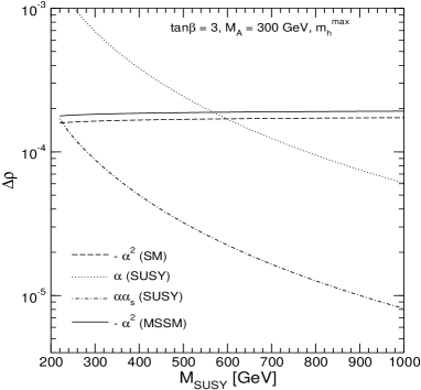
Figure 4: The contribution of the leading ${\cal O}(\alpha_{t}^{2})$ MSSM corrections, $\Delta\rho_{1,\mathrm{Higgs}}^{\mathrm{SUSY}}$, eq. (A.1), is shown as a function of $M_{\rm SUSY}$ for $M_{A}=300\,\,\mathrm{GeV}$ and $\tan\beta=3$ (left plot) or $\tan\beta=40$ (right plot) in the $m_{h}^{\rm max}$ scenario. $\Delta\rho_{1,\mathrm{Higgs}}^{\mathrm{SUSY}}$ is compared with the leading ${\cal O}(\alpha_{t}^{2})$ SM contribution and with the leading MSSM corrections originating from the $\tilde{t}/\tilde{b}$ sector of ${\cal O}(\alpha)$ and ${\cal O}(\alpha\alpha_{s})$. Both ${\cal O}(\alpha_{t}^{2})$ contributions are negative and are for comparison shown with reversed sign. In the right plot the ${\cal O}(\alpha_{t}^{2})$ corrections differ by about $1.5\times 10^{-7}$, which is not visible in the plot.

   

Figure 5: The contribution of the leading ${\cal O}(\alpha_{t}^{2})$ MSSM corrections, $\Delta\rho_{1,\mathrm{Higgs}}^{\mathrm{SUSY}}$, is shown as a function of $m_{h}$ for $\tan\beta=3$ (left plot) and for $\tan\beta=40$ (right plot) in the $m_{h}^{\rm max}$ and the no-mixing scenario. $\Delta\rho_{1,\mathrm{Higgs}}^{\mathrm{SUSY}}$ is compared with the leading ${\cal O}(\alpha_{t}^{2})$ SM contribution.

   

Figure 6: The ${\cal O}(\alpha_{t}^{2})$ MSSM contribution to $\Delta\rho$ in the $m_{h}^{\rm max}$ and the no-mixing scenario is compared with the corresponding SM result with $M_{H}^{\mathrm{SM}}=m_{h}$. $m_{h}$ is obtained in the left (right) plot from varying $M_{A}$ from $100\,\,\mathrm{GeV}$ to $3000(300)\,\,\mathrm{GeV}$, while keeping $\tan\beta$ fixed at $\tan\beta=3(40)$.

In Fig. 6 the decoupling behavior for large $M_{A}$ of $\Delta\rho^{\mathrm{SUSY}}_{1,{\rm Higgs}}$ is analyzed numerically. Since $M_{A}$ is the only non-SM scale that directly enters $\Delta\rho^{\mathrm{SUSY}}_{1,{\rm Higgs}}$, the result should become SM-like once $M_{A}$ is taken to very large values. This is shown in the $m_{h}^{\rm max}$ and the no-mixing scenario for $\tan\beta$ fixed to $\tan\beta=3(40)$ in the left (right) plot of Fig. 6. The SM value of $\Delta\rho^{\mathrm{SM}}_{1,{\rm Higgs}}$ is obtained for $M_{H}^{\mathrm{SM}}=m_{h}$. While for the small $\tan\beta$ value the decoupling is very slow and is reached only for $M_{A}\;\raisebox{-3.00003pt}{$\stackrel{{\scriptstyle\displaystyle>}}{{\sim}}$}\;3\,\,\mathrm{TeV}$, for the large $\tan\beta$ value $\Delta\rho^{\mathrm{SUSY}}_{1,{\rm Higgs}}$ decouples already for very small $M_{A}$ values. This numerical behavior is analogous to the analytical result described in Sect. 3 for the $m_{h}\to 0$ limit. However, it should also be noted that for small values of $M_{A}$ the behavior of the SM and the MSSM contributions is very different. While the SM contribution depends sensitively on $M_{H}^{\mathrm{SM}}$, in the MSSM for $M_{A}\;\raisebox{-3.00003pt}{$\stackrel{{\scriptstyle\displaystyle>}}{{\sim}}$}\;100\,\,\mathrm{GeV}$ (corresponding to $m_{h}\;\raisebox{-3.00003pt}{$\stackrel{{\scriptstyle\displaystyle>}}{{\sim}}$}\;90\,\,\mathrm{GeV}$, see Fig. 5) the dependence on the Higgs boson masses is much less pronounced, see in particular the right plot of Fig. 6.

4.1.2 Effects on precision observables

In this section the numerical effect of the ${\cal O}(\alpha_{t}^{2})$ corrections on the electroweak precision observables, $M_{W}$ and $\sin^{2}\theta_{\mathrm{eff}}$ is analyzed. In addition to the MSSM ${\cal O}(\alpha_{t}^{2})$ correction to $\delta M_{W}$ and $\delta\sin^{2}\theta_{\mathrm{eff}}$, we also present the effective change from the SM result (where the SM Higgs boson mass has been set to $m_{h}$) to our new MSSM result.

   

Figure 7: The absolute ${\cal O}(\alpha_{t}^{2})$ MSSM contribution and the effective change in $\delta M_{W}$ is shown for $M_{\rm SUSY}=1000\,\,\mathrm{GeV}$ in the $m_{h}^{\rm max}$ scenario. The other parameters are $\mu=200\,\,\mathrm{GeV},A_{b}=A_{t}$. $m_{h}$ is obtained in the left (right) plot from varying $M_{A}$ from $50\,\,\mathrm{GeV}$ to $1000\,\,\mathrm{GeV}$, while keeping $\tan\beta$ fixed at $\tan\beta=3,40$ (from varying $\tan\beta$ from 2 to 40, while keeping $M_{A}$ fixed at $M_{A}=100,300\,\,\mathrm{GeV}$.)

   

Figure 8: The absolute ${\cal O}(\alpha_{t}^{2})$ MSSM contribution and the effective change in $\delta\sin^{2}\theta_{\mathrm{eff}}$ is shown for $M_{\rm SUSY}=1000\,\,\mathrm{GeV}$ in the $m_{h}^{\rm max}$ scenario. The other parameters are $\mu=200\,\,\mathrm{GeV},A_{b}=A_{t}$. $m_{h}$ is obtained in the left (right) plot from varying $M_{A}$ from $50\,\,\mathrm{GeV}$ to $1000\,\,\mathrm{GeV}$, while keeping $\tan\beta$ fixed at $\tan\beta=3,40$ (from varying $\tan\beta$ from 2 to 40, while keeping $M_{A}$ fixed at $M_{A}=100,300\,\,\mathrm{GeV}$.)

In Fig. 7 the absolute contribution and the effective change for the $W$ boson mass is presented. For the numerical evaluation we have chosen the $m_{h}^{\rm max}$ benchmark scenario (where $M_{\rm SUSY}=1000\,\,\mathrm{GeV}$). In the left plot $\tan\beta$ is fixed to $\tan\beta=3,40$, while $M_{A}$ is varied from $50\,\,\mathrm{GeV}$ to $1000\,\,\mathrm{GeV}$, resulting in the Higgs boson mass $m_{h}$. The effect of the ${\cal O}(\alpha_{t}^{2})$ MSSM contributions on $\delta M_{W}$ amounts up to $-12\,\,\mathrm{MeV}$. For large $M_{A}$ and/or large $\tan\beta$ it saturates at about $-10\,\,\mathrm{MeV}$. The effective change in $M_{W}$ is significantly smaller. It amounts up to $-3\,\,\mathrm{MeV}$ and goes to zero for large $M_{A}$ as expected from the decoupling behavior. In the right plot of Fig. 7 $\delta M_{W}$ is shown as a function of $\tan\beta$. $M_{A}$ is kept fixed to $M_{A}=100,300\,\,\mathrm{GeV}$. The effect of $\Delta\rho^{\mathrm{SUSY}}_{1,\mathrm{Higgs}}$ saturates for large $\tan\beta$. For a small ${\cal CP}$-odd Higgs boson mass, $M_{A}=100\,\,\mathrm{GeV}$, a shift of $-2\,\,\mathrm{MeV}$ in $M_{W}$ remains also in the limit of large $\tan\beta$, since the two Higgs doublet sector does not decouple from the MSSM. For large $M_{A}$, $M_{A}=300\,\,\mathrm{GeV}$, for nearly all $\tan\beta$ values the effective change in $M_{W}$ is small.

The absolute contribution and the effective change for $\delta\sin^{2}\theta_{\mathrm{eff}}$ is shown in Fig. 8 for the same parameters as in Fig. 7. The absolute effect is around $+6\times 10^{-5}$. The effective change ranges between $+3\times 10^{-5}$ for small $\tan\beta$ and small $M_{A}$ and approximately zero for large $\tan\beta$ and large $M_{A}$.

The effects of the ${\cal O}(\alpha_{t}^{2})$ MSSM corrections in $M_{W}$ and $\sin^{2}\theta_{\mathrm{eff}}$ discussed above are smaller than the current experimental errors, $\delta M_{W}^{\rm exp}=34\,\,\mathrm{MeV}$ and $\delta\sin^{2}\theta_{\mathrm{eff}}^{\rm exp}=17\times 10^{-5}$ [30]. However, their inclusion is crucial in order to reduce the theoretical uncertainties from unknown higher order corrections within the MSSM to a similar level as in the SM of $\delta M_{W}^{\rm theo}\approx\pm 5\,\,\mathrm{MeV}$ and $\delta\sin^{2}\theta_{\mathrm{eff}}^{\rm theo}\approx\pm 7\times 10^{-5}$ [31, 32]. Achieving this level of theoretical accuracy will be mandatory in particular in view of the prospective accuracies at a future linear collider running on the $Z$ peak and the $WW$ threshold (GigaZ), $\delta M_{W}^{\rm exp,fut}\approx 7\,\,\mathrm{MeV}$ and $\delta\sin^{2}\theta_{\mathrm{eff}}^{\rm exp,fut}\approx 1.3\times 10^{-5}$ [33, 34, 32].

4.2 The ${\cal O}(\alpha_{t}^{2})$, ${\cal O}(\alpha_{t}\alpha_{b})$, and ${\cal O}(\alpha_{b}^{2})$ contributions

In this section the numerical effect of the ${\cal O}(\alpha_{t}^{2})$, ${\cal O}(\alpha_{t}\alpha_{b})$, and ${\cal O}(\alpha_{b}^{2})$ corrections on $\Delta\rho$ is analyzed. As discussed in Sect. 2.4, for these corrections is was necessary to employ the Higgs sector restrictions as given in eqs. (24) and (25). This implies that the couplings of the lightest ${\cal CP}$-even Higgs boson to gauge bosons and SM fermions are SM-like. Corrections enhanced by $\tan\beta$ thus arise only from the heavy Higgs bosons, while the contribution from the lightest ${\cal CP}$-even Higgs boson resembles the SM one.

   

Figure 9: The ${\cal O}(\alpha_{t}^{2})$, ${\cal O}(\alpha_{t}\alpha_{b})$, and ${\cal O}(\alpha_{b}^{2})$ MSSM contribution to $\Delta\rho$ in the $m_{h}^{\rm max}$ and the no-mixing scenario is compared with the corresponding SM result with $M_{H}^{\mathrm{SM}}=m_{h}$. In the left plot $\tan\beta$ is fixed to $\tan\beta=40$, while $M_{A}$ is varied from $50\,\,\mathrm{GeV}$ to $1000\,\,\mathrm{GeV}$. In the right plot $M_{A}$ is set to $300\,\,\mathrm{GeV}$, while $\tan\beta$ is varied. The bottom quark mass is set to $m_{b}=4.25\,\,\mathrm{GeV}$.

In Fig. 9 we show the result for the ${\cal O}(\alpha_{t}^{2})$, ${\cal O}(\alpha_{t}\alpha_{b})$, and ${\cal O}(\alpha_{b}^{2})$ MSSM contributions to $\Delta\rho$ in the $m_{h}^{\rm max}$ and the no-mixing scenario, compared with the corresponding SM result with $M_{H}^{\mathrm{SM}}=m_{h}$. In the left plot $\tan\beta$ is fixed to $\tan\beta=40$ and $M_{A}$ is varied from $50\,\,\mathrm{GeV}$ to $1000\,\,\mathrm{GeV}$. In the right plot $M_{A}$ is fixed to $M_{A}=300\,\,\mathrm{GeV}$, while $\tan\beta$ is varied.

For large $\tan\beta$ the ${\cal O}(\alpha_{t}\alpha_{b})$ and ${\cal O}(\alpha_{b}^{2})$ contributions yield a significant effect from the heavy Higgs bosons in the loops, entering with the other sign than the ${\cal O}(\alpha_{t}^{2})$ corrections, while the contribution of the lightest Higgs boson is SM-like. As one can see in Fig. 9, for large $\tan\beta$ the MSSM contribution to $\Delta\rho$ is smaller than the SM value. For large values of $M_{A}$, the SM result is recovered. The effective change in the predictions for the precision observables from the ${\cal O}(\alpha_{t}\alpha_{b})$ and ${\cal O}(\alpha_{b}^{2})$ corrections can exceed the one from the ${\cal O}(\alpha_{t}^{2})$ corrections. It can amount up to $\delta M_{W}\approx+5\,\,\mathrm{MeV}$ and $\delta\sin^{2}\theta_{\mathrm{eff}}\approx-3\times 10^{-5}$ for $\tan\beta=40$.

5 Constraints on the top Yukawa coupling in the SM and the MSSM

The $\Delta\rho^{\alpha_{t,b}^{2}}_{1,{\rm Higgs}}$ corrections in the SM and the MSSM are of particular interest, since these are the leading corrections in which the top and bottom Yukawa couplings, i.e. the coupling of Higgs bosons to top and bottom quarks, enter the predictions for the electroweak precision observables. Thus, the electroweak precision tests of the SM and the MSSM provide some sensitivity to the Yukawa couplings in these models.

In order to exemplify this sensitivity, we use a simple approach in which we treat the top Yukawa coupling in the SM and the MSSM as a free parameter. While a complete calculation of top and bottom contributions, as discussed in the previous sections, requires the relation between the Yukawa coupling and fermion mass within the SM and the MSSM, this relation is not formally needed if one restricts to the top contributions only. Numerically, this is an excellent approximation within the SM and also in the MSSM for not too large $\tan\beta$.

In the following we analyze the sensitivity to the top Yukawa coupling in the SM and the MSSM. Since in the MSSM contributions beyond the $\Delta\rho^{\alpha_{t}^{2}}_{1,{\rm Higgs}}$ corrections are not yet known, for this comparison we restrict the SM contributions also to the leading electroweak $\Delta\rho^{\alpha_{t}^{2}}_{1,{\rm Higgs}}$ term [12], neglecting the formally subleading electroweak two-loop corrections to the precision observables [31], which can, however, be of similar size.

Fig. 10 shows the effect of varying the top Yukawa coupling in the SM and the MSSM for the precision observables $M_{W}$ and $\sin^{2}\theta_{\mathrm{eff}}$ in comparison with the current experimental precision. The allowed 68% and 95% C.L. contours are indicated in the figure. The Yukawa coupling is scaled in the following way,

$$y_{t}=x\,y_{t}^{\mathrm{SM}},\quad 0\leq x\leq 3,$$ (32)

and analogously in the MSSM. A shift of this kind in the relation between a fermion mass and the corresponding Yukawa coupling can occur for instance in the MSSM (see e.g. Ref. [35]),

$$y_{t}=\frac{\sqrt{2}\,m_{t}}{v\,\sin\beta\hskip 2.84526pt}\,\frac{1}{1+\Delta_{t}}~{},$$ (33)

where $\Delta_{t}$ is induced by SUSY loop corrections. Here we do not assume any particular scenario but use the variation of the top Yukawa coupling only for demonstrating the sensitivity to this parameter.

Figure 10: The effect of scaling the top Yukawa coupling in the SM (upper plot) and the MSSM (lower plot) for the precision observables $M_{W}$ and $\sin^{2}\theta_{\mathrm{eff}}$ is shown in comparison with the current experimental precision. The variation with $m_{t}$ and $\Delta\alpha_{\rm had}$ is shown within their current experimental errors. For the SM evaluation, $M_{H}^{\mathrm{SM}}$ has been set to the conservative value of $M_{H}^{\mathrm{SM}}=114\,\,\mathrm{GeV}$ (see text). For the MSSM evaluation the parameters are $M_{\rm SUSY}=1000\,\,\mathrm{GeV}$, $X_{t}=2000\,\,\mathrm{GeV}$, $M_{A}=175\,\,\mathrm{GeV}$, $\tan\beta=3$ and $\mu=200\,\,\mathrm{GeV}$, resulting in $m_{h}\approx 114\,\,\mathrm{GeV}$. The obtained upper bounds are $y_{t}<1.3\,y_{t}^{\mathrm{SM}}$ and $y_{t}<1.7\,y_{t}^{\mathrm{MSSM}}$ for $m_{t}=174.3\,\,\mathrm{GeV}$ as well as $y_{t}<2.2\,y_{t}^{\mathrm{SM}}$ and $y_{t}<2.5\,y_{t}^{\mathrm{MSSM}}$ for $m_{t}=179.4\,\,\mathrm{GeV}$, all at the 95% C.L.

For the evaluation of $M_{W}$ and $\sin^{2}\theta_{\mathrm{eff}}$ in the SM and the MSSM, we take into account the complete one-loop results as well as the leading two-loop ${\cal O}(\alpha\alpha_{s})$ and ${\cal O}(\alpha_{t}^{2})$ corrections (as discussed in Refs. [32, 36]). Since the SM prediction deviates more from the experimental central value for increasing values of $M_{H}^{\mathrm{SM}}$, we have chosen in the figure $M_{H}^{\mathrm{SM}}=114\,\,\mathrm{GeV}$ [37] as a conservative value. The current $1\sigma$ uncertainties in $m_{t}$ and $\Delta\alpha_{\rm had}$ are also taken into account, as indicated in the figures. Varying the SM top Yukawa coupling (upper plot) yields an upper bound of $y_{t}<1.3\,y_{t}^{\mathrm{SM}}$ for $m_{t}=174.3\,\,\mathrm{GeV}$ and of $y_{t}<2.2\,y_{t}^{\mathrm{SM}}$ for $m_{t}=179.4\,\,\mathrm{GeV}$, both at the 95% C.L. These relatively strong bounds are of course related to the fact that the theory prediction in the SM shows some deviation from the current experimental central value.

The lower plot of Fig. 10 shows the analogous analysis in the MSSM for one particular example of SUSY parameters. We have chosen a large value of $M_{\rm SUSY}$, $M_{\rm SUSY}=1000\,\,\mathrm{GeV}$, in order to justify the approximation of neglecting the ${\cal O}(\alpha_{t}^{2})$ contributions from SUSY loops. The other parameters are $X_{t}=2000\,\,\mathrm{GeV}$, $M_{A}=175\,\,\mathrm{GeV}$, $\tan\beta=3$ and $\mu=200\,\,\mathrm{GeV}$, resulting in $m_{h}\approx 114\,\,\mathrm{GeV}$ (for comparison with the SM case). The SUSY contributions to $M_{W}$ and $\sin^{2}\theta_{\mathrm{eff}}$ lead to a somewhat better agreement between the theory prediction and experiment and consequently to somewhat weaker bounds on $y_{t}$. In this example we find $y_{t}<1.7\,y_{t}^{\mathrm{MSSM}}$ for $m_{t}=174.3\,\,\mathrm{GeV}$ and $y_{t}<2.5\,y_{t}^{\mathrm{MSSM}}$ for $m_{t}=179.4\,\,\mathrm{GeV}$, both at the 95% C.L.

In order to demonstrate the sensitivity of future colliders for the determination of the top Yukawa coupling from electroweak precision observables, we list in Tab. 1 the bounds on $y_{t}$ obtainable at the LHC and a future LC with GigaZ option [34]. Here we assume that the future experimental central values of $M_{W}$ and $\sin^{2}\theta_{\mathrm{eff}}$ agree with the theory predictions for $y_{t}/y_{t}^{\mathrm{SM}}=1$ and $y_{t}/y_{t}^{\mathrm{MSSM}}=1$, respectively. An accuracy in the indirect determination of $y_{t}$ of about 40% can be achieved with the GigaZ precision at the 95% C.L. This is similar to the accuracy achievable from the $t\bar{t}$ threshold measurements, see Ref. [39]. The results in Tab. 1 are the same for the SM and our SUSY example, since the only difference (after assuming that the future experimental central values of $M_{W}$ and $\sin^{2}\theta_{\mathrm{eff}}$ agree perfectly with the SM or MSSM predictions) are the relatively small deviations at ${\cal O}(\alpha_{t}^{2})$ between the SM and the MSSM shown in Figs. 7, 8.

	LHC ($\delta m_{t}=2\,\,\mathrm{GeV}$)	LHC ($\delta m_{t}=1\,\,\mathrm{GeV}$)	LC/GigaZ
$y_{t}/y_{t}^{\mathrm{SM}}$	2.5	2.3	1.4
$y_{t}/y_{t}^{\mathrm{MSSM}}$	2.5	2.3	1.4

Table 1: Sensitivity to the top Yukawa coupling at future colliders: For the LHC we assume $\delta m_{t}=2\,\,\mathrm{GeV}$ or $1\,\,\mathrm{GeV}$, $\delta M_{W}=15\,\,\mathrm{MeV}$, $\delta\sin^{2}\theta_{\mathrm{eff}}=17\times 10^{-5}$ [32, 38], while for LC/GigaZ we use $\delta m_{t}=0.1\,\,\mathrm{GeV}$, $\delta M_{W}=7\,\,\mathrm{MeV}$ and $\delta\sin^{2}\theta_{\mathrm{eff}}=1.3\times 10^{-5}$ [33, 34, 32]. For $\Delta\alpha_{\rm had}$ we assume a future uncertainty of $\delta\Delta\alpha_{\rm had}=5\times 10^{-5}$. The bounds on $y_{t}/y_{t}^{\mathrm{SM}}$ and $y_{t}/y_{t}^{\mathrm{MSSM}}$ are given at the 95% C.L., assuming that the theory predictions agree with the experimental central values for $M_{W}$ and $\sin^{2}\theta_{\mathrm{eff}}$ for $y_{t}/y_{t}^{\mathrm{SM},\mathrm{SUSY}}=1$. The SUSY parameters are chosen as for Fig. 10.

6 Conclusions

We have calculated the leading ${\cal O}(\alpha_{t}^{2})$, ${\cal O}(\alpha_{t}\alpha_{b})$, and ${\cal O}(\alpha_{b}^{2})$ corrections to $\Delta\rho$ in the MSSM in the limit of heavy squarks. The analytical results for arbitrary values of the lightest ${\cal CP}$-even Higgs boson mass have been presented. While for the ${\cal O}(\alpha_{t}^{2})$ result all parameters in the ${\cal CP}$-even Higgs sector could be kept arbitrary, for the full result further tree-level relations had to be employed, which lead to SM-like couplings of the lightest ${\cal CP}$-even Higgs boson to gauge bosons and SM fermions.

Numerically we compared the effect of the new MSSM contribution with the leading ${\cal O}(\alpha_{t}^{2})$ SM contribution. For small $\tan\beta$, it is sufficient to restrict to the ${\cal O}(\alpha_{t}^{2})$ corrections. Their numerical effect is always larger than the ${\cal O}(\alpha_{t}^{2})$ SM contribution. The corrections to the precision observables $M_{W}$ and $\sin^{2}\theta_{\mathrm{eff}}$ amount up to $-12\,\,\mathrm{MeV}$ for $M_{W}$ and about $+6\times 10^{-5}$ for $\sin^{2}\theta_{\mathrm{eff}}$. The effective change from the SM ${\cal O}(\alpha_{t}^{2})$ result with $M_{H}^{\mathrm{SM}}=m_{h}$ is smaller. It amounts up to $-3\,\,\mathrm{MeV}$ for $M_{W}$ and $+2\times 10^{-5}$ for $\sin^{2}\theta_{\mathrm{eff}}$. This effective change goes to zero for large $M_{A}$, i.e. the non-SM contribution decouples.

The ${\cal O}(\alpha_{t}\alpha_{b})$ and ${\cal O}(\alpha_{b}^{2})$ contributions become important for large $\tan\beta$. They enter with a different sign than the ${\cal O}(\alpha_{t}^{2})$ corrections and can overcompensate the latter. For large $\tan\beta$ the effective change in the predictions for the precision observables from the whole ${\cal O}(\alpha_{t}^{2})$, ${\cal O}(\alpha_{t}\alpha_{b})$, and ${\cal O}(\alpha_{b}^{2})$ corrections can amount up to $\delta M_{W}\approx+5\,\,\mathrm{MeV}$ and $\delta\sin^{2}\theta_{\mathrm{eff}}\approx-3\times 10^{-5}$. For large $M_{A}$ also in this case the SM result is recovered.

The MSSM corrections to the electroweak precision observables discussed here are important in order to reduce the theoretical uncertainties from unknown higher order corrections within the MSSM to a similar level as currently reached for the SM. Achieving this level of theoretical accuracy will be mandatory in particular in view of the prospective accuracies at a future linear collider running on the $Z$ peak and the $WW$ threshold.

We have furthermore discussed the sensitivity of the electroweak precision observables to the top Yukawa coupling, which enters at the two-loop level. Varying the SM top Yukawa coupling and requiring consistency with the present experimental values of $M_{W}$ and $\sin^{2}\theta_{\mathrm{eff}}$ at the 95% C.L. yields an upper bound of $y_{t}<1.3\,y_{t}^{\mathrm{SM}}$ for $m_{t}=174.3\,\,\mathrm{GeV}$. This bound can be relaxed within the MSSM, where additional contributions from SUSY loops to the electroweak precision observables can lead to a better agreement with the experimental data. We have also analyzed the sensitivity of future colliders for the determination of the top Yukawa coupling from electroweak precision observables, assuming that the future experimental central values of $M_{W}$ and $\sin^{2}\theta_{\mathrm{eff}}$ agree with the theory predictions for unmodified Yukawa couplings. An accuracy in the indirect determination of $y_{t}$ of about 40% can be achieved with GigaZ precision at the 95% C.L., which is similar to the accuracy achievable from $t\bar{t}$ threshold measurements.

Acknowledgements

S.H. acknowledges hospitality and financial support by CERN and IPPP Durham, where part of the work has been done. G.W. thanks the Max-Planck Institut für Physik in Munich for the hospitality offered to him during the final stage of this work. We thank W. Hollik for useful discussions and T. Hahn for technical help. This work has been supported by the European Community’s Human Potential Programme under contract HPRN-CT-2000-00149 Physics at Colliders.

Appendix

Appendix A Analytical results or arbitrary values of $m_{h}$

A.1 The result for the ${\cal O}(\alpha_{t}^{2})$ contributions for arbitrary parameters in the ${\cal CP}$-even Higgs sector

We give here the analytical result for the ${\cal O}(\alpha_{t}^{2})$ contributions where $m_{h}$, $m_{H}$ and $\alpha$ are kept as arbitrary parameters, see Sect. 2.4. The full result for the ${\cal O}(\alpha_{t}^{2})$ contributions can conveniently be expressed in terms of

$$A\equiv\frac{m_{t}^{2}}{M_{A}^{2}},\quad H\equiv\frac{m_{t}^{2}}{m_{H}^{2}},\quad h\equiv\frac{m_{t}^{2}}{m_{h}^{2}}~{}.$$ (34)

We furthermore use the abbreviations $s_{x}\equiv\sin x,c_{x}\equiv\cos x$ and

$$\Lambda_{x} \equiv 3A^{2}(1-6x+10x^{2})-4Ax(1-5x+7x^{2})+x^{2}(1-4x+6x^{2})$$

$$\Lambda^{\prime}_{x} \equiv A^{2}(-1+12x+12x^{2})-2Ax(-1+10x+4x^{2})+x^{2}(-1+8x)$$

$$Y_{x} \equiv 2x(-1+4x)\left[A(1-4x)-x\right]$$

$$P_{3} \equiv 2A^{2}(-1+4A)(h-H)\Big{[}2A^{3}+A^{2}(-1+2h+2H)-6AhH+hH\Big{]}$$

$$P_{4} \equiv 2A(-1+4A)(h-H)\Big{[}20A^{4}-2A^{3}(5+6h+6H)$$

$$+A^{2}(1+8H+8h+4hH)-A(h+H+6hH)+hH\Big{]}$$

$$P^{\prime}_{4} \equiv -2A(-1+4A)(h-H)\Big{[}18A^{4}-A^{3}(9+14h+14H)$$

$$+A^{2}(1+8H+8h+10hH)-A(h+H+7hH)+hH\Big{]}$$

$$P_{5} \equiv 4A^{5}+A^{4}(54+136h)-2A^{3}(17+108h+54h^{2})$$ (35)

$$+A^{2}(5+94h+146h^{2})-2Ah(6+29h)+7h^{2}~{}.$$

The two-loop contribution to the $\rho\,$-parameter then reads:

$$\Delta\rho_{1,\mathrm{Higgs}}^{\mathrm{SUSY}}=3\,\frac{G_{F}^{2}}{128\,\pi^{4}}\,m_{t}^{4}\frac{1}{s_{\beta}^{2}}\;\times$$

$$\Bigg{\{}{\rm Li}_{2}\left((1-\sqrt{1-4\,H}\,)/2\right)\frac{2}{\sqrt{1-4\,H}\,(A-H)^{2}H^{2}}\Bigg{[}s_{\alpha}^{2}\Lambda_{H}+s_{\beta}s_{\alpha}(s_{\beta}s_{\alpha}+c_{\beta}c_{\alpha})Y_{H}$$

$$\left[s_{\beta}c_{\beta}(s_{\beta}c_{\beta}+s_{\alpha}c_{\alpha})+s_{\beta}s_{\alpha}(s_{\beta}s_{\alpha}+c_{\beta}c_{\alpha})+2s_{\beta}^{3}s_{\alpha}(s_{\beta}s_{\alpha}+c_{\beta}c_{\alpha})\right]2H^{3}(-1+4H)+\Bigg{]}$$

$$+ {\rm Li}_{2}\left((1-\sqrt{1-4\,h}\,)/2\right)\frac{2}{\sqrt{1-4\,h}\,(A-h)^{2}h^{2}}\Bigg{[}c_{\alpha}^{2}\Lambda_{h}+s_{\beta}c_{\alpha}(s_{\beta}c_{\alpha}-s_{\alpha}c_{\beta})Y_{h}$$

$$-\left[-2s_{\alpha}c_{\alpha}s_{\beta}c_{\beta}(1+s_{\beta}^{2})+s_{\beta}^{2}(1+c_{\alpha}^{2})+s_{\beta}^{4}(1-2s_{\alpha}^{2})\right]2h^{3}(1-4h)\Bigg{]}$$

$$+ {\rm Li}_{2}\left((1-\sqrt{1-4\,A}\,)/2\right)\frac{2c_{\beta}}{\sqrt{1-4\,A}\,(1-4A)A^{2}(A-h)^{2}(A-H)^{2}}$$

$$\Bigg{[}s_{\alpha}c_{\alpha}s_{\beta}P_{4}-\left[2s_{\alpha}c_{\alpha}s_{\beta}^{3}+s_{\beta}^{2}c_{\beta}(1-2s_{\alpha}^{2})\right]P_{3}+c_{\beta}(A-H)^{2}P_{5}+c_{\beta}s_{\alpha}^{2}P^{\prime}_{4}\Bigg{]}$$

$$+ {\rm Li}_{2}\left(1-\frac{1}{H}\right)\frac{(H-1)^{2}}{(A-H)^{2}H^{2}}\Bigg{[}s_{\alpha}^{2}\left[A^{2}(-3+6H)-4A(-1+H)H-H^{2}\right]$$

$$+\left[s_{\beta}^{2}(1+s_{\alpha}^{2})-s_{\beta}^{4}(1-2s_{\alpha}^{2})+2s_{\beta}c_{\beta}s_{\alpha}c_{\alpha}(1+s_{\beta}^{2})\right]2H^{3}$$

$$+s_{\beta}s_{\alpha}(s_{\beta}s_{\alpha}+c_{\beta}c_{\alpha})2H(A(1-4H)-H)\Bigg{]}$$

$$- {\rm Li}_{2}\left(1-\frac{1}{h}\right)\frac{(h-1)^{2}}{(A-h)^{2}h^{2}}\Bigg{[}\left[2s_{\beta}c_{\beta}(1+s_{\beta}^{2})s_{\alpha}c_{\alpha}-s_{\beta}^{2}(1+c_{\alpha}^{2})-s_{\beta}^{4}(1-2s_{\alpha}^{2})\right]2h^{3}$$

$$+s_{\beta}c_{\alpha}(c_{\beta}s_{\alpha}-s_{\beta}c_{\alpha})2h(A(1-4h)-h)+c_{\alpha}^{2}\left[A^{2}(3-6h)+4Ah(-1+h)+h^{2}\right]\Bigg{]}$$

$$- {\rm Li}_{2}\left(1-\frac{1}{A}\right)\frac{c_{\beta}}{A^{2}(A-h)^{2}(A-H)^{2}}\Bigg{[}s_{\alpha}c_{\alpha}s_{\beta}2(A-1)A(h-H)\Big{[}2A^{4}-7A^{3}$$

$$+A^{2}(1+5h+5H-2hH)-A(h+H+3hH)+hH\Big{]}$$

$$+\left[2s_{\alpha}c_{\alpha}s_{\beta}^{3}+s_{\beta}^{2}c_{\beta}(1-2s_{\alpha}^{2})\right]2(A-1)A^{2}(h-H)\Big{[}A^{3}+A^{2}(1-2h-2H)$$

$$+3AhH-hH\Big{]}+c_{\beta}(A-H)^{2}\Big{[}A^{4}(-3+6h)-4A^{3}(1+3h+h^{2})$$

$$+A^{2}(3+22h+11h^{2})-8Ah(1+2h)+5h^{2}\Big{]}+c_{\beta}s_{\alpha}^{2}(-2)(A-1)A(h-H)$$

$$\Big{[}3A^{4}-2A^{3}(3+h+H)+A^{2}(1+5h+5H+hH)-A(h+H+4hH)+hH\Big{]}\Bigg{]}$$

$$+ \log^{2}(h)\frac{1}{2\sqrt{1-4\,h}\,(A-h)^{2}h^{2}}\Bigg{[}\Big{\{}2s_{\beta}s_{\alpha}\left[s_{\beta}s_{\alpha}+c_{\beta}c_{\alpha}(1+s_{\beta}^{2})\right]$$

$$-s_{\beta}^{2}\left[2+s_{\alpha}^{2}+s_{\beta}^{2}(1-2s_{\alpha}^{2})\right]\Big{\}}2h^{3}(1-4h)+s_{\beta}s_{\alpha}c_{\alpha}c_{\beta}2h(-1+4h)(A(-1+4h)+h)$$

$$+c_{\alpha}^{2}\Lambda_{h}+s_{\beta}^{2}c_{\alpha}^{2}Y_{h}\Bigg{]}$$

$$+ \log^{2}(H)\frac{1}{2\sqrt{1-4\,H}\,(A-H)^{2}H^{2}}\Bigg{[}s_{\alpha}^{2}\Lambda_{H}+\Big{\{}s_{\beta}^{2}\left[1+s_{\alpha}^{2}-s_{\beta}^{2}(1-2s_{\alpha}^{2})\right]+$$

$$2s_{\beta}c_{\beta}s_{\alpha}c_{\alpha}(1+s_{\beta}^{2})\Big{\}}2H^{3}(-1+4H)+s_{\beta}s_{\alpha}(s_{\beta}s_{\alpha}+c_{\beta}c_{\alpha})Y_{H}\Bigg{]}$$

$$+ \log^{2}(A)\frac{c_{\beta}}{2(1-4A)^{2}A^{2}(A-h)^{2}(A-H)^{2}}\Bigg{[}s_{\beta}s_{\alpha}c_{\alpha}\sqrt{1-4\,A}\,P_{4}$$

$$+s_{\beta}^{2}\left[-2s_{\beta}s_{\alpha}c_{\alpha}-c_{\beta}(1-2s_{\alpha}^{2})\right]\sqrt{1-4\,A}\,P_{3}+c_{\beta}(A-H)^{2}\Big{[}2(1-4A)^{2}(A-h)^{2}$$

$$+\sqrt{1-4\,A}\,P_{5}\Big{]}+c_{\beta}s_{\alpha}^{2}\sqrt{1-4\,A}\,P^{\prime}_{4}\Bigg{]}$$

$$+ \log(h)\frac{1}{2h^{2}(A-h)^{2}}\Bigg{[}\left[-2s_{\beta}c_{\beta}(1+s_{\beta}^{2})s_{\alpha}c_{\alpha}+s_{\beta}^{2}c_{\alpha}^{2}+s_{\beta}^{2}(1+s_{\beta}^{2}(1-2s_{\alpha}^{2}))\right]4h^{4}$$

$$+s_{\beta}c_{\alpha}(c_{\beta}s_{\alpha}-s_{\beta}c_{\alpha})4h^{2}(A(1+4h)-h)+c_{\alpha}^{2}\Lambda^{\prime}_{h}\Bigg{]}$$

$$+ \log(H)\frac{1}{2H^{2}(A-H)^{2}}\Bigg{[}s_{\alpha}^{2}\Lambda^{\prime}_{H}+\Big{[}s_{\beta}^{2}+s_{\beta}s_{\alpha}(s_{\beta}s_{\alpha}+c_{\beta}c_{\alpha})-s_{\beta}^{4}(1-2s_{\alpha}^{2})$$

$$+s_{\beta}c_{\beta}s_{\alpha}c_{\alpha}(1+2s_{\beta}^{2})\Big{]}4H^{4}+s_{\beta}s_{\alpha}(s_{\beta}s_{\alpha}+c_{\beta}c_{\alpha})4H^{2}(-A(1+4H)+H)\Bigg{]}$$

$$+ \log(A)\frac{1}{2A^{2}(-1+4A)(A-h)^{2}(A-H)^{2}}\Bigg{[}-(A-H)^{2}\Big{[}A^{4}(-76+48h)$$

$$+A^{3}(32+156h-32h^{2})+A^{2}(-3-68h-84h^{2})+6Ah(1+6h)-3h^{2}\Big{]}$$

$$+s_{\alpha}^{2}4A^{2}(-1+4A)(h-H)\left[3A^{3}+A^{2}(1-2h-2H)-A(h+H-hH)+hH\right]$$

$$+s_{\beta}^{2}\Big{[}4A^{6}(-19+8h+4H)-4A^{5}(-8-40h-37H+24hH+8H^{2})$$

$$+A^{4}(-3-64H-68h-68H^{2}-92h^{2}-312hH+16h^{2}H+96hH^{2})$$

$$+A^{3}(6H+6h+32H^{2}+36h^{2}+136hH+180h^{2}H+144hH^{2}-32h^{2}H^{2})$$

$$+A^{2}(-3h^{2}-3H^{2}-12hH-72h^{2}H-68hH^{2}-84h^{2}H^{2})+6AhH(h+H+6hH)$$

$$-3h^{2}H^{2}\Big{]}+s_{\beta}^{2}s_{\alpha}^{2}(-4A^{2})(-1+4A)(h-H)\Big{[}A^{3}+A^{2}(1+2h+2H)$$

$$-A(h+H+5hH)+hH\Big{]}+s_{\beta}^{4}(1-2s_{\alpha}^{2})4A^{3}(-1+4A)(h-H)\Big{[}A^{2}-2A(h+H)$$

$$+3hH\Big{]}+s_{\beta}c_{\beta}s_{\alpha}c_{\alpha}(-4A^{2})(-1+4A)(h-H)\left[2A^{3}+A^{2}-A(h+H+2hH)+hH\right]$$

$$+s_{\beta}^{3}c_{\beta}s_{\alpha}c_{\alpha}(-8A^{3})(-1+4A)(h-H)\left[A^{2}-2A(h+H)+3hH\right]\Bigg{]}$$

$$+ \log\left[(1-\sqrt{1-4\,h}\,)/2\right]\frac{1}{\sqrt{1-4\,h}\,(A-h)^{2}h^{2}}\Bigg{[}-c_{\alpha}^{2}\Lambda_{h}+\Big{[}-2s_{\beta}^{2}$$

$$+s_{\beta}s_{\alpha}(s_{\beta}s_{\alpha}+c_{\beta}c_{\alpha})-s_{\beta}^{4}(1-2s_{\alpha}^{2})+s_{\beta}c_{\beta}s_{\alpha}c_{\alpha}(1+2s_{\beta}^{2})\Big{]}2h^{3}(-1+4h)$$

$$+\left[s_{\beta}s_{\alpha}(s_{\beta}s_{\alpha}+c_{\beta}c_{\alpha})-s_{\beta}^{2}\right]Y_{h}\Bigg{]}$$

$$- \log\left[(1-\sqrt{1-4\,H}\,)/2\right]\frac{1}{\sqrt{1-4\,H}\,(A-H)^{2}H^{2}}\Bigg{[}s_{\alpha}^{2}\Lambda_{H}+\Big{[}s_{\beta}^{2}(1+s_{\alpha}^{2})$$

$$-s_{\beta}^{4}(1-2s_{\alpha}^{2})+2s_{\beta}c_{\beta}s_{\alpha}c_{\alpha}(1+s_{\beta}^{2})\Big{]}2H^{3}(-1+4H)+s_{\beta}s_{\alpha}(s_{\beta}s_{\alpha}+c_{\beta}c_{\alpha})Y_{H}\Bigg{]}$$

$$- \log\left[(1-\sqrt{1-4\,A}\,)/2\right]\frac{c_{\beta}}{(1-4A)\sqrt{1-4\,A}\,A^{2}(A-h)^{2}(A-H)^{2}}\Bigg{[}s_{\beta}s_{\alpha}c_{\alpha}P_{4}$$

$$+s_{\beta}^{2}\left[-2s_{\beta}s_{\alpha}c_{\alpha}-c_{\beta}(1-2s_{\alpha}^{2})\right]P_{3}+c_{\beta}(A-H)^{2}P_{5}+c_{\beta}s_{\alpha}^{2}P^{\prime}_{4}\Bigg{]}$$

$$+ \log\left(\frac{1-\sqrt{1-4\,h}\,}{1+\sqrt{1-4\,h}\,}\right)\frac{c_{\alpha}^{2}\sqrt{1-4\,h}\,(1-4h)}{2h^{2}}$$

$$+ \log\left(\frac{1-\sqrt{1-4\,H}\,}{1+\sqrt{1-4\,H}\,}\right)\frac{s_{\alpha}^{2}\sqrt{1-4\,H}\,(1-4H)}{2H^{2}}$$

$$+ \log\left(\frac{1-\sqrt{1-4\,A}\,}{1+\sqrt{1-4\,A}\,}\right)\frac{c_{\beta}^{2}\sqrt{1-4\,A}\,}{2A^{2}}$$

$$+ \log\left(|-1+1/A|\right)\frac{-c_{\beta}^{2}(A-1)^{2}}{A^{2}}$$

$$+ \frac{1}{6(1-4A)^{2}A^{2}h^{2}H^{2}(A-h)^{2}(A-H)^{2}(-1+4h)(-1+4H)}\times$$

$$\Bigg{[}6(1-4A)^{2}AhH(A-h)(A-H)(-1+4h)(-1+4H)\times$$

$$\Bigg{(}H(A-H)\left[A^{2}(-4+25h)-Ah(7+23h)+11h^{2}\right]+s_{\alpha}^{2}(-2A)(h-H)$$

$$\left[2A^{2}+A(-2H-2h+hH)+2hH\right]+s_{\beta}^{2}hH\Big{[}A^{2}(11-4h+2H)$$

$$+A(-11H-11h+2hH)+11hH\Big{]}+s_{\beta}^{2}s_{\alpha}^{2}Hh(6A^{2})(h-H)$$

$$+s_{\beta}^{4}(1-2s_{\alpha}^{2})(2A^{2}hH(h-H))+s_{\beta}c_{\beta}^{3}s_{\alpha}c_{\alpha}4A^{2}hH(h-H)\Bigg{)}$$

$$+ \pi^{2}\Bigg{(}(1-4A)^{2}(1-4h)(1-4H)(A-h)^{2}(A-H)^{2}h^{2}H^{2}\Big{\{}2A^{2}(h-H)\Big{[}(-1+2s_{\alpha}^{2})s_{\beta}^{4}$$

$$+2s_{\alpha}c_{\alpha}s_{\beta}(1+s_{\beta}^{2})c_{\beta}\Big{]}+2+s_{\beta}^{2}\left[-2+A^{2}\{3+2h(-2+s_{\alpha}^{2})-2H(1+s_{\alpha}^{2})\}\right]\Big{\}}$$

$$+(1-4A)^{2}A^{2}h^{2}(A-h)^{2}(-1+4h)\sqrt{1-4\,H}\,\Big{\{}s_{\alpha}^{2}\Lambda_{H}+s_{\beta}s_{\alpha}(s_{\beta}s_{\alpha}+c_{\beta}c_{\alpha})Y_{H}$$

$$+\left[s_{\beta}^{2}(1+s_{\alpha}^{2})-s_{\beta}^{4}(1-2s_{\alpha}^{2})+2s_{\beta}c_{\beta}s_{\alpha}c_{\alpha}(1+s_{\beta}^{2})\right]2H^{3}(-1+4H)\Big{\}}$$

$$-(1-4A)^{2}A^{2}H^{2}(A-H)^{2}(-1+4H)\sqrt{1-4\,h}\,\Big{\{}-c_{\alpha}^{2}\Lambda_{h}+s_{\beta}c_{\alpha}(-s_{\beta}c_{\alpha}+c_{\beta}s_{\alpha})Y_{h}$$

$$+\left[s_{\beta}^{2}s_{\alpha}^{2}-2s_{\beta}^{2}-s_{\beta}^{4}(1-2s_{\alpha}^{2})+2s_{\beta}c_{\beta}s_{\alpha}c_{\alpha}(1+s_{\beta}^{2})\right]2h^{3}(-1+4h)\Big{\}}$$

$$-\left[\sqrt{1-4\,A}\,h^{2}H^{2}(1-4h)(1-4H)\right]\Big{\{}(A-H)^{2}P_{5}+s_{\alpha}^{2}P^{\prime}_{4}+s_{\beta}^{2}\Big{[}-4A^{7}$$

$$+A^{6}(-54-152h+24H)+2A^{5}(17+114h+48H+46h^{2}+6H^{2}+136hH)$$

$$-A^{4}(5+96h+66H+142h^{2}+58H^{2}+432hH+168h^{2}H+184hH^{2})$$

$$+2A^{3}(6h+5H+29h^{2}+17H^{2}+94hH+136h^{2}H+118hH^{2}+54h^{2}H^{2})$$

$$-A^{2}(7h^{2}+5H^{2}+24hH+114h^{2}H+96hH^{2}+146h^{2}H^{2})$$

$$+2AhH(6H+7h+29hH)-7h^{2}H^{2}\Big{]}+s_{\beta}^{2}s_{\alpha}^{2}2A(-1+4A)(h-H)\Big{[}22A^{4}$$

$$-A^{3}(11+10h+10H)+A^{2}(1+8h+8H-2hH)-A(h+H+5hH)+hH\Big{]}$$

$$+s_{\beta}^{3}(s_{\beta}-2s_{\beta}s_{\alpha}^{2}-2c_{\beta}s_{\alpha}c_{\alpha})P_{3}+s_{\beta}c_{\beta}s_{\alpha}c_{\alpha}P_{4}\Big{\}}\Bigg{)}\Bigg{]}\Bigg{\}}.$$

A.2 The result for the ${\cal O}(\alpha_{t}^{2})$, ${\cal O}(\alpha_{t}\alpha_{b})$ and ${\cal O}(\alpha_{b}^{2})$ corrections

In the following we list the full result for the ${\cal O}(\alpha_{t}^{2})$, ${\cal O}(\alpha_{t}\alpha_{b})$ and ${\cal O}(\alpha_{b}^{2})$ corrections. As explained in Sect. 2.4, it has been obtained by using the Higgs sector relations eqs. (24) and (25). We give this result for arbitrary space–time dimension $D$, using the shorthands

$$\Delta_{i,j,k,l}=i+j\,D+k\,D^{2}+l\,D^{3},\quad\Delta_{i,j,k}=i+j\,D+k\,D^{2}~{}.$$ (37)

The result is expressed in terms of the one-loop scalar integrals $A_{0}(m)$ and $B_{0}(p^{2},m_{1},m_{2})$ as defined in Ref. [8] and the scalar two-loop vacuum integral $T_{134}(m_{1}^{2},m_{2}^{2},m_{3}^{2})$ as defined in Ref. [22].

$$\Delta\rho_{1,{\rm Higgs}}^{\mathrm{SUSY},\alpha_{t,b}^{2}}\;=\;\frac{3\,G_{F}^{2}}{(4\pi)^{4}D}\times$$ (38)

$${}\Bigg{[}\;A_{0}(m_{t})\,\Bigg{\{}8\,(D-2)\,m_{t}^{2}\,B_{0}(m_{b}^{2},0,m_{t})$$

$${}-\frac{16\,(D-2)\,m_{b}^{2}\,\left(M_{A}^{2}-2\,m_{b}^{2}\right)\,m_{t}^{2}\,s_{\beta}^{2}\,B_{0}(m_{b}^{2},M_{A},m_{b})}{c_{\beta}^{2}\,{\left(m_{b}^{2}-m_{t}^{2}\right)}^{2}}+\frac{8\,(D-2)\,m_{t}^{2}}{c_{\beta}^{2}\,{\left(m_{b}^{2}-m_{t}^{2}\right)}^{2}\,s_{\beta}^{2}}$$

$${}\Big{(}c_{\beta}^{4}\,m_{t}^{4}+m_{b}^{4}\,s_{\beta}^{4}+m_{b}^{2}\,m_{t}^{2}\,\left(1+2\,s_{\beta}^{2}-2\,s_{\beta}^{4}\right)-M_{A}^{2}\,\left(c_{\beta}^{4}\,m_{t}^{2}+m_{b}^{2}\,s_{\beta}^{4}\right)\Big{)}\,B_{0}(m_{b}^{2},M_{A},m_{t})$$

$${}+\frac{8\,(D-2)\,m_{b}^{2}\,\left(4\,m_{b}^{2}-m_{h}^{2}\right)\,m_{t}^{2}\,B_{0}(m_{b}^{2},m_{b},m_{h})}{{\left(m_{b}^{2}-m_{t}^{2}\right)}^{2}}$$

$${}-\frac{(D-2)\,\mathop{\mathrm{Re}}(B_{0}(m_{t}^{2},0,m_{b}))\,\left((D-2)\,D\,m_{b}^{4}-2\,(D-4)\,D\,m_{b}^{2}\,m_{t}^{2}+m_{t}^{4}\,\Delta_{8,-6,1}\right)}{m_{t}^{2}}$$

$${}-\frac{(D-2)}{c_{\beta}^{2}\,{\left(m_{b}^{2}\,m_{t}-m_{t}^{3}\right)}^{2}\,s_{\beta}^{2}}\Big{[}\Big{(}c_{\beta}^{4}\,m_{t}^{4}+m_{b}^{4}\,s_{\beta}^{4}+m_{b}^{2}\,m_{t}^{2}\,\left(1+2\,s_{\beta}^{2}-2\,s_{\beta}^{4}\right)-M_{A}^{2}\,\left(c_{\beta}^{4}\,m_{t}^{2}+m_{b}^{2}\,s_{\beta}^{4}\right)\Big{)}\,$$

$${}\mathop{\mathrm{Re}}(B_{0}(m_{t}^{2},M_{A},m_{b}))\,\left((D-2)\,D\,m_{b}^{4}-2\,(D-4)\,D\,m_{b}^{2}\,m_{t}^{2}+m_{t}^{4}\,\Delta_{8,-6,1}\right)\Big{]}$$

$${}+\frac{2\,c_{\beta}^{2}\,(D-2)\,\left(M_{A}^{2}-2\,m_{t}^{2}\right)\,B_{0}(m_{t}^{2},M_{A},m_{t})}{{\left(m_{b}^{2}-m_{t}^{2}\right)}^{2}\,s_{\beta}^{2}}\Big{(}(D-2)\,D\,m_{b}^{4}-2\,(D-4)\,D\,m_{b}^{2}\,m_{t}^{2}$$

$${}+m_{t}^{4}\,\Delta_{8,-6,1}\Big{)}+\frac{(D-2)\,\left(m_{h}^{2}-4\,m_{t}^{2}\right)\,B_{0}(m_{t}^{2},m_{h},m_{t})}{{\left(m_{b}^{2}-m_{t}^{2}\right)}^{2}}\Bigg{\}}$$

$${}\left((D-2)\,D\,m_{b}^{4}-2\,(D-4)\,D\,m_{b}^{2}\,m_{t}^{2}+m_{t}^{4}\,\Delta_{8,-6,1}\right)$$

$$+A_{0}(m_{h})\,A_{0}(m_{t})\,\frac{1}{m_{h}^{2}\,\left(m_{h}-2\,m_{t}\right)\,\left(m_{h}+2\,m_{t}\right)\,\left(-m_{b}^{2}+m_{t}^{2}\right)}\Big{(}-48\,m_{b}^{4}\,\left(m_{h}^{2}-4\,m_{t}^{2}\right)$$

$${}+m_{t}^{2}\,\left(192\,m_{t}^{4}+4\,m_{h}^{2}\,m_{t}^{2}\,\Delta_{-40,24,-13,2}-m_{h}^{4}\,\Delta_{-24,16,-8,1}\right)$$

$${}+m_{b}^{2}\,\left(-384\,m_{t}^{4}-4\,m_{h}^{2}\,m_{t}^{2}\,\Delta_{-20,16,-9,2}+m_{h}^{4}\,\Delta_{8,8,-4,1}\right)\Big{)}$$

$$+\frac{2\,{A_{0}(m_{t})}^{2}}{c_{\beta}^{2}\,\left(-3+D\right)\,\left(M_{A}-2\,m_{t}\right)\,\left(M_{A}+2\,m_{t}\right)\,\left(-m_{h}+2\,m_{t}\right)\,\left(m_{h}+2\,m_{t}\right)\,\left(-m_{b}^{2}+m_{t}^{2}\right)\,s_{\beta}^{2}}$$

$${}\Bigg{\{}\Big{[}-2\,m_{t}^{2}\,\Bigg{(}(D-2)\,m_{b}^{2}\,\Bigg{(}-4\,m_{t}^{2}\,\left(s_{\beta}^{2}\,\left(-3\,D^{3}+\Delta_{-58,17,10}\right)+s_{\beta}^{4}\,\Delta_{22,-17,3}+\Delta_{12,8,-13,3}\right)$$

$${}+m_{h}^{2}\,\left(s_{\beta}^{2}\,\left(-4\,D^{3}+\Delta_{-52,6,16}\right)+\Delta_{12,8,-13,3}+s_{\beta}^{4}\,\Delta_{16,-6,-3,1}\right)\Bigg{)}$$

$${}-c_{\beta}^{2}\,m_{t}^{2}\,\Big{(}m_{h}^{2}\,\left(3\,D^{4}+s_{\beta}^{2}\,\left(5\,D^{3}-D^{4}+\Delta_{128,-108,16}\right)+\Delta_{-72,60,30,-23}\right)$$

$${}+4\,m_{t}^{2}\,\left(-3\,D^{4}+s_{\beta}^{2}\,\left(3\,D^{3}+\Delta_{-140,136,-39}\right)+\Delta_{72,-60,-30,23}\right)\Big{)}\Bigg{)}$$

$${}+M_{A}^{2}\,\Bigg{(}m_{h}^{2}\,\Big{(}-c_{\beta}^{2}\,m_{t}^{2}\,\left(D^{4}+s_{\beta}^{2}\,\left(2\,D^{3}+\Delta_{52,-32,-1}\right)+\Delta_{-24,8,24,-11}\right)$$

$${}+(D-2)\,m_{b}^{2}\,\left(\left(-10+3\,D\right)\,s_{\beta}^{4}+D\,\Delta_{6,-5,1}-s_{\beta}^{2}\,\Delta_{2,5,-5,1}\right)\Big{)}$$

$${}+2\,m_{t}^{2}\Big{(}(D-2)\,m_{b}^{2}\,\left(-2\,D\,\Delta_{6,-5,1}+s_{\beta}^{2}\,\Delta_{10,-1,-4,1}+s_{\beta}^{4}\,\Delta_{14,5,-6,1}\right)$$

$${}-m_{t}^{2}\,\left(s_{\beta}^{2}\,\left(D^{4}+\Delta_{-164,108,27,-18}\right)-2\,\left(D^{4}+\Delta_{-24,8,24,-11}\right)+s_{\beta}^{4}\,\left(D^{4}+\Delta_{116,-92,21,-4}\right)\right)\Big{)}\Bigg{)}\Big{]}\Bigg{\}}$$

$$+\frac{2\,{A_{0}(m_{b})}^{2}}{c_{\beta}^{2}\,\left(-3+D\right)\,\left(M_{A}-2\,m_{b}\right)\,\left(M_{A}+2\,m_{b}\right)\,\left(2\,m_{b}-m_{h}\right)\,\left(2\,m_{b}+m_{h}\right)\,\left(m_{b}^{2}-m_{t}^{2}\right)\,s_{\beta}^{2}}$$

$${}\Bigg{\{}M_{A}^{2}\,\Big{[}2\,m_{b}^{4}\,s_{\beta}^{2}\,\left(-3\,D^{4}+s_{\beta}^{2}\,\left(-4\,D^{3}+D^{4}+\Delta_{116,-92,21}\right)+\Delta_{-68,76,-69,26}\right)$$

$${}-(D-2)\,m_{h}^{2}\,m_{t}^{2}\,\left(4\,\left(-3+D\right)+\left(-10+3\,D\right)\,s_{\beta}^{4}+s_{\beta}^{2}\,\Delta_{22,-1,-5,1}\right)$$

$${}+m_{b}^{2}\,\Big{(}m_{h}^{2}\,s_{\beta}^{2}\,\left(D^{4}+s_{\beta}^{2}\,\left(-2\,D^{3}+\Delta_{-52,32,1}\right)+\Delta_{28,-24,23,-9}\right)$$

$${}-2\,(D-2)\,m_{t}^{2}\,\left(-8\,\left(-3+D\right)+s_{\beta}^{4}\,\Delta_{14,5,-6,1}-s_{\beta}^{2}\,\Delta_{38,9,-16,3}\right)\Big{)}\Big{]}$$

$${}+2\,m_{b}^{2}\,\Big{[}(D-2)\,m_{h}^{2}\,m_{t}^{2}\,\left(8\,\left(-3+D\right)+2\,s_{\beta}^{2}\,\Delta_{10,3,-5,1}+s_{\beta}^{4}\,\Delta_{16,-6,-3,1}\right)$$

$${}+4\,m_{b}^{4}\,s_{\beta}^{2}\,\left(3\,D^{4}+s_{\beta}^{2}\,\left(3\,D^{3}+\Delta_{-140,136,-39}\right)+\Delta_{68,-76,69,-26}\right)$$

$${}+m_{b}^{2}\,\Big{(}-4\,(D-2)\,m_{t}^{2}\,\left(8\,\left(-3+D\right)+s_{\beta}^{4}\,\Delta_{22,-17,3}+s_{\beta}^{2}\,\Delta_{14,17,-16,3}\right)$$

$${}+m_{h}^{2}\,s_{\beta}^{2}\,\left(-2\,\left(D^{4}+\Delta_{28,-24,23,-9}\right)+s_{\beta}^{2}\,\left(-D^{4}+\Delta_{128,-108,16,5}\right)\right)\Big{)}\Big{]}\Bigg{\}}$$

$$+A_{0}(m_{b})\,\Bigg{\{}(D-2)\,D\,\left(\frac{2-D}{m_{b}^{2}}-\frac{4\,\left(\left(-1+\frac{2}{D}\right)\,m_{b}^{2}+m_{t}^{2}\right)}{{\left(m_{b}^{2}-m_{t}^{2}\right)}^{2}}\right)$$

$${}\left(4\,m_{b}^{2}\,m_{t}^{2}-\frac{\left(M_{A}^{2}-m_{b}^{2}-m_{t}^{2}\right)\,\left(c_{\beta}^{4}\,m_{t}^{2}+m_{b}^{2}\,s_{\beta}^{4}\right)}{c_{\beta}^{2}\,s_{\beta}^{2}}\right)\,B_{0}(m_{b}^{2},M_{A},m_{t})$$

$${}+8\,(D-2)\,m_{b}^{2}\,\mathop{\mathrm{Re}}(B_{0}(m_{t}^{2},0,m_{b}))+\frac{8\,(D-2)\,m_{b}^{2}}{c_{\beta}^{2}\,{\left(m_{b}^{2}-m_{t}^{2}\right)}^{2}\,s_{\beta}^{2}}\,\Big{(}c_{\beta}^{4}\,m_{t}^{4}+m_{b}^{4}\,s_{\beta}^{4}$$

$${}+m_{b}^{2}\,m_{t}^{2}\,\left(1+2\,s_{\beta}^{2}-2\,s_{\beta}^{4}\right)-M_{A}^{2}\,\left(c_{\beta}^{4}\,m_{t}^{2}+m_{b}^{2}\,s_{\beta}^{4}\right)\Big{)}\,\mathop{\mathrm{Re}}(B_{0}(m_{t}^{2},M_{A},m_{b}))$$

$${}-\frac{16\,c_{\beta}^{2}\,(D-2)\,m_{b}^{2}\,m_{t}^{2}\,\left(M_{A}^{2}-2\,m_{t}^{2}\right)\,B_{0}(m_{t}^{2},M_{A},m_{t})}{{\left(m_{b}^{2}-m_{t}^{2}\right)}^{2}\,s_{\beta}^{2}}$$

$${}-\frac{8\,(D-2)\,m_{b}^{2}\,m_{t}^{2}\,\left(m_{h}^{2}-4\,m_{t}^{2}\right)\,B_{0}(m_{t}^{2},m_{h},m_{t})}{{\left(m_{b}^{2}-m_{t}^{2}\right)}^{2}}$$

$${}-\frac{(D-2)\,B_{0}(m_{b}^{2},0,m_{t})\,\left(-2\,(D-4)\,D\,m_{b}^{2}\,m_{t}^{2}+(D-2)\,D\,m_{t}^{4}+m_{b}^{4}\,\Delta_{8,-6,1}\right)}{m_{b}^{2}}$$

$${}+\frac{2\,(D-2)\,\left(M_{A}^{2}-2\,m_{b}^{2}\right)\,s_{\beta}^{2}\,B_{0}(m_{b}^{2},M_{A},m_{b})}{c_{\beta}^{2}\,{\left(m_{b}^{2}-m_{t}^{2}\right)}^{2}}\Big{(}-2\,(D-4)\,D\,m_{b}^{2}\,m_{t}^{2}$$

$${}+(D-2)\,D\,m_{t}^{4}+m_{b}^{4}\,\Delta_{8,-6,1}\Big{)}-\frac{(D-2)\,\left(4\,m_{b}^{2}-m_{h}^{2}\right)\,B_{0}(m_{b}^{2},m_{b},m_{h})}{{\left(m_{b}^{2}-m_{t}^{2}\right)}^{2}}$$

$${}\Big{(}-2\,(D-4)\,D\,m_{b}^{2}\,m_{t}^{2}+(D-2)\,D\,m_{t}^{4}+m_{b}^{4}\,\Delta_{8,-6,1}\Big{)}-\frac{A_{0}(m_{h})}{m_{h}^{2}\,\left(4\,m_{b}^{2}-m_{h}^{2}\right)\,\left(m_{b}^{2}-m_{t}^{2}\right)}$$

$${}\Big{(}192\,m_{b}^{6}+4\,m_{b}^{4}\,\left(-96\,m_{t}^{2}+m_{h}^{2}\,\Delta_{-40,24,-13,2}\right)+m_{b}^{2}\,\big{(}192\,m_{t}^{4}-m_{h}^{4}\,\Delta_{-24,16,-8,1}$$

$${}-4\,m_{h}^{2}\,m_{t}^{2}\,\Delta_{-20,16,-9,2}\big{)}+m_{h}^{2}\,m_{t}^{2}\,\left(-48\,m_{t}^{2}+m_{h}^{2}\,\Delta_{8,8,-4,1}\right)\Big{)}$$

$${}+\frac{A_{0}(m_{t})}{s_{\beta}^{2}c_{\beta}^{2}\,m_{b}^{2}\,m_{t}^{2}\,{\left(M_{A}^{2}-(m_{t}-m_{b})^{2}\right)}^{2}\,{\left(M_{A}^{2}-(m_{t}+m_{b})^{2}\right)}^{2}\,\left(m_{b}^{2}-m_{t}^{2}\right)}$$

$${}\Big{[}{\left(m_{b}^{2}-m_{t}^{2}\right)}^{3}\,\Bigg{(}c_{\beta}^{2}\,{(D-2)}^{2}\,D\,m_{t}^{8}+{(D-2)}^{2}\,D\,m_{b}^{8}\,s_{\beta}^{2}+m_{b}^{4}\,m_{t}^{4}\,\Big{(}-{\left(10-3\,D\right)}^{2}\,D$$

$${}+96\,(D-2)\,s_{\beta}^{2}-96\,(D-2)\,s_{\beta}^{4}\Big{)}+m_{b}^{6}\,m_{t}^{2}\,\left({(D-2)}^{2}\,D+48\,(D-2)\,s_{\beta}^{4}-2\,s_{\beta}^{2}\,\Delta_{-48,60,-32,5}\right)$$

$${}+m_{b}^{2}\,m_{t}^{6}\,\left(48\,(D-2)\,s_{\beta}^{4}+D\,\Delta_{-68,60,-9}+2\,s_{\beta}^{2}\,\Delta_{48,12,-32,5}\right)\Bigg{)}$$

$${}+M_{A}^{8}\,\Bigg{(}-c_{\beta}^{2}\,{(D-2)}^{2}\,D\,m_{t}^{6}+{(D-2)}^{2}\,D\,m_{b}^{6}\,s_{\beta}^{2}+m_{b}^{2}\,m_{t}^{4}\,\Big{(}-32\,\left(-1+D\right)+s_{\beta}^{2}\,\Delta_{-160,188,-68,11}$$

$${}-4\,s_{\beta}^{4}\,\Delta_{-32,40,-18,3}\Big{)}+m_{b}^{4}\,m_{t}^{2}\,\left({(D-2)}^{2}\,D+4\,s_{\beta}^{4}\,\Delta_{-32,40,-18,3}+s_{\beta}^{2}\,\Delta_{96,-132,76,-13}\right)\Bigg{)}$$

$${}-4\,M_{A}^{6}\,\Bigg{(}-c_{\beta}^{2}\,{(D-2)}^{2}\,D\,m_{t}^{8}+{(D-2)}^{2}\,D\,m_{b}^{8}\,s_{\beta}^{2}-4\,m_{b}^{4}\,m_{t}^{4}\,\left(-1+2\,s_{\beta}^{2}\right)\,\Delta_{8,-10,1}$$

$${}+m_{b}^{2}\,m_{t}^{6}\,\left(-4\,\Delta_{-4,4,1}+s_{\beta}^{2}\,\Delta_{-128,148,-52,9}-2\,s_{\beta}^{4}\,\Delta_{-56,68,-30,5}\right)$$

$${}+m_{b}^{6}\,m_{t}^{2}\,\Big{(}{(D-2)}^{2}\,D+2\,s_{\beta}^{4}\,\Delta_{-56,68,-30,5}+s_{\beta}^{2}\,\Delta_{96,-124,68,-11}\Big{)}\Bigg{)}$$

$${}-4\,M_{A}^{2}\,{\left(m_{b}^{2}-m_{t}^{2}\right)}^{2}\,\Bigg{(}-c_{\beta}^{2}\,{(D-2)}^{2}\,D\,m_{t}^{8}+{(D-2)}^{2}\,D\,m_{b}^{8}\,s_{\beta}^{2}$$

$${}+4\,m_{b}^{4}\,m_{t}^{4}\,\left(-1+2\,s_{\beta}^{2}\right)\,\Delta_{-4,18,-8,1}+m_{b}^{6}\,m_{t}^{2}\,\left({(D-2)}^{2}\,D+4\,s_{\beta}^{4}\,\Delta_{-24,20,-6,1}+s_{\beta}^{2}\,\Delta_{96,-116,60,-9}\right)$$

$${}+m_{b}^{2}\,m_{t}^{6}\,\left(4\,D\,\Delta_{8,-8,1}-4\,s_{\beta}^{4}\,\Delta_{-24,20,-6,1}-s_{\beta}^{2}\,\Delta_{96,-44,-12,1}\right)\Bigg{)}$$

$${}+2\,M_{A}^{4}\,\Bigg{(}-3\,c_{\beta}^{2}\,{(D-2)}^{2}\,D\,m_{t}^{10}+3\,{(D-2)}^{2}\,D\,m_{b}^{10}\,s_{\beta}^{2}-2\,m_{b}^{6}\,m_{t}^{4}\,\Big{(}s_{\beta}^{4}\,\left(17\,D^{3}+\Delta_{-72,204,-118}\right)$$

$${}-4\,s_{\beta}^{2}\,\left(5\,D^{3}+\Delta_{-32,78,-36}\right)+\Delta_{-40,84,-26,3}\Big{)}+2\,m_{b}^{4}\,m_{t}^{6}\,\Big{(}16-24\,D+s_{\beta}^{4}\,\Delta_{-72,204,-118,17}$$

$${}-2\,s_{\beta}^{2}\,\Delta_{-8,48,-46,7}\Big{)}+m_{b}^{2}\,m_{t}^{8}\,\Big{(}s_{\beta}^{2}\,\left(13\,D^{3}+\Delta_{-320,292,-68}\right)+s_{\beta}^{4}\,\left(-22\,D^{3}+\Delta_{304,-328,132}\right)$$

$${}+\Delta_{16,24,-52,6}\Big{)}+m_{b}^{8}\,m_{t}^{2}\,\left(3\,{(D-2)}^{2}\,D+s_{\beta}^{4}\,\Delta_{-304,328,-132,22}+s_{\beta}^{2}\,\Delta_{288,-364,196,-31}\right)\Bigg{)}\Big{]}\Bigg{\}}$$

$$+A_{0}(M_{A})\,\Bigg{\{}-A_{0}(m_{t})\frac{1}{c_{\beta}^{2}\,\left(M_{A}-2\,m_{t}\right)\,{\left(M_{A}+m_{b}-m_{t}\right)}^{2}\,m_{t}^{2}\,{\left(M_{A}-m_{b}+m_{t}\right)}^{2}}$$

$${}\frac{1}{{\left(-M_{A}+m_{b}+m_{t}\right)}^{2}\,{\left(M_{A}+m_{b}+m_{t}\right)}^{2}\,\left(M_{A}+2\,m_{t}\right)\,\left(-m_{b}^{2}+m_{t}^{2}\right)\,s_{\beta}^{2}}$$

$${}\Bigg{\{}M_{A}^{10}\,\Bigg{(}-{(D-2)}^{2}\,D\,m_{b}^{4}\,s_{\beta}^{4}+m_{b}^{2}\,m_{t}^{2}\,\left(-3\,{(D-2)}^{2}\,D+6\,{(D-2)}^{2}\,D\,s_{\beta}^{2}-2\,s_{\beta}^{4}\,\Delta_{-24,20,-2,1}\right)$$

$${}+c_{\beta}^{4}\,m_{t}^{4}\,\Delta_{16,12,-24,3}\Bigg{)}+2\,M_{A}^{8}\,\Bigg{(}2\,{(D-2)}^{2}\,D\,m_{b}^{6}\,s_{\beta}^{4}+m_{b}^{4}\,m_{t}^{2}\,\Big{(}6\,{(D-2)}^{2}\,D-10\,{(D-2)}^{2}\,D\,s_{\beta}^{2}$$

$${}+s_{\beta}^{4}\,\Delta_{-72,68,-14,7}\Big{)}+m_{b}^{2}\,m_{t}^{4}\,\left(s_{\beta}^{4}\,\left(6\,D^{3}+\Delta_{-192,136,16}\right)-4\,s_{\beta}^{2}\,\left(5\,D^{3}+\Delta_{-4,8,-5}\right)+\Delta_{-24,12,-2,9}\right)$$

$${}-c_{\beta}^{4}\,m_{t}^{6}\,\Delta_{88,20,-94,15}\Bigg{)}+4\,m_{t}^{2}\,{\left(m_{b}^{2}-m_{t}^{2}\right)}^{2}\,\Bigg{(}{(D-2)}^{2}\,D\,m_{b}^{8}\,s_{\beta}^{4}+m_{b}^{6}\,m_{t}^{2}\,\Big{(}2\,{(D-2)}^{2}\,\left(1+2\,D\right)$$

$${}-4\,s_{\beta}^{2}\,\Delta_{8,-2,-3,1}-s_{\beta}^{4}\,\Delta_{8,52,-46,5}\Big{)}-2\,c_{\beta}^{4}\,m_{t}^{8}\,\Delta_{20,-4,-13,3}+m_{b}^{4}\,m_{t}^{4}\,\Big{(}-4\,s_{\beta}^{2}\,\Delta_{-52,112,-45,3}$$

$${}+s_{\beta}^{4}\,\Delta_{-24,100,-54,1}-2\,\Delta_{44,20,-39,7}\Big{)}+m_{b}^{2}\,m_{t}^{6}\,\Big{(}s_{\beta}^{4}\,\left(9\,D^{3}+\Delta_{72,-60,-14}\right)+4\,s_{\beta}^{2}\,\Delta_{-64,114,-35,1}$$

$${}+\Delta_{120,-360,166,-16}\Big{)}\Bigg{)}-2\,M_{A}^{6}\,\Bigg{(}3\,{(D-2)}^{2}\,D\,m_{b}^{8}\,s_{\beta}^{4}+m_{b}^{2}\,m_{t}^{6}\,\Big{(}s_{\beta}^{4}\,\left(17\,D^{3}+\Delta_{-648,588,2}\right)$$

$${}+s_{\beta}^{2}\,\left(-44\,D^{3}+\Delta_{256,-288,8}\right)+\Delta_{-192,36,92,9}\Big{)}+m_{b}^{6}\,m_{t}^{2}\,\Big{(}9\,{(D-2)}^{2}\,D-12\,{(D-2)}^{2}\,D\,s_{\beta}^{2}$$

$${}+s_{\beta}^{4}\,\Delta_{-88,68,-10,11}\Big{)}+m_{b}^{4}\,m_{t}^{4}\,\Big{(}s_{\beta}^{4}\,\left(17\,D^{3}+\Delta_{-248,108,78}\right)-4\,s_{\beta}^{2}\,\left(10\,D^{3}+\Delta_{20,-16,-5}\right)$$

$${}+\Delta_{-24,32,-46,30}\Big{)}-2\,c_{\beta}^{4}\,m_{t}^{8}\,\Delta_{148,4,-131,24}\Bigg{)}+2\,M_{A}^{4}\,\Bigg{(}2\,{(D-2)}^{2}\,D\,m_{b}^{10}\,s_{\beta}^{4}+m_{b}^{4}\,m_{t}^{6}\,\Big{(}4\,s_{\beta}^{2}\,\Big{(}19\,D^{3}$$

$${}+\Delta_{132,64,-143}\Big{)}-2\,s_{\beta}^{4}\,\left(37\,D^{3}+\Delta_{168,236,-298}\right)+\Delta_{-328,84,114,3}\Big{)}+m_{b}^{8}\,m_{t}^{2}\,\Big{(}6\,{(D-2)}^{2}\,D$$

$${}-6\,{(D-2)}^{2}\,D\,s_{\beta}^{2}+s_{\beta}^{4}\,\Delta_{-56,20,6,7}\Big{)}+m_{b}^{2}\,m_{t}^{8}\,\Big{(}2\,s_{\beta}^{4}\,\left(49\,D^{3}+\Delta_{-304,612,-248}\right)$$

$${}-4\,s_{\beta}^{2}\,\left(38\,D^{3}+\Delta_{44,152,-139}\right)+\Delta_{-8,-164,82,25}\Big{)}+m_{b}^{6}\,m_{t}^{4}\,\Big{(}4\,s_{\beta}^{4}\,\left(9\,D^{3}+\Delta_{-24,52,-14}\right)$$

$${}-4\,s_{\beta}^{2}\,\left(14\,D^{3}+\Delta_{52,16,-41}\right)+\Delta_{8,20,-66,35}\Big{)}-c_{\beta}^{4}\,m_{t}^{10}\,\Delta_{440,-36,-342,69}\Bigg{)}$$

$${}-M_{A}^{2}\,\Big{[}{(D-2)}^{2}\,D\,m_{b}^{12}\,s_{\beta}^{4}+2\,m_{b}^{6}\,m_{t}^{6}\,\Big{(}4\,s_{\beta}^{4}\,\left(7\,D^{3}+\Delta_{-104,232,-102}\right)+2\,s_{\beta}^{2}\,\left(59\,D^{3}+\Delta_{432,4,-276}\right)$$

$${}+\Delta_{-368,-276,408,-65}\Big{)}+m_{b}^{10}\,m_{t}^{2}\,\left(3\,{(D-2)}^{2}\,D-2\,{(D-2)}^{2}\,D\,s_{\beta}^{2}+8\,s_{\beta}^{4}\,\Delta_{-4,2,-1,1}\right)$$

$${}+m_{b}^{8}\,m_{t}^{4}\,\left(s_{\beta}^{4}\,\left(-7\,D^{3}+\Delta_{32,-268,244}\right)-2\,s_{\beta}^{2}\,\left(47\,D^{3}+\Delta_{192,156,-212}\right)+\Delta_{64,44,-124,47}\right)$$

$${}+m_{b}^{4}\,m_{t}^{8}\,\left(s_{\beta}^{4}\,\left(-221\,D^{3}+\Delta_{1088,-2900,1380}\right)+4\,s_{\beta}^{2}\,\Delta_{-16,-196,140,1}+\Delta_{160,1272,-1040,142}\right)$$

$${}-c_{\beta}^{4}\,m_{t}^{12}\,\Delta_{608,-92,-428,93}+m_{b}^{2}\,m_{t}^{10}\,\Big{(}s_{\beta}^{2}\,\left(-330\,D^{3}+\Delta_{-2496,1272,968}\right)$$

$${}+8\,s_{\beta}^{4}\,\left(32\,D^{3}+\Delta_{44,150,-153}\right)+\Delta_{1120,-1892,444,31}\Big{)}\Big{]}\Bigg{\}}$$

$${}+A_{0}(m_{b})\frac{1}{c_{\beta}^{2}\,m_{b}^{2}\,\left(M_{A}^{2}-4\,m_{b}^{2}\right)\,{\left(M_{A}+m_{b}-m_{t}\right)}^{2}\,{\left(M_{A}-m_{b}+m_{t}\right)}^{2}\,{\left(-M_{A}+m_{b}+m_{t}\right)}^{2}}$$

$${}\frac{1}{{\left(M_{A}+m_{b}+m_{t}\right)}^{2}\,\left(m_{b}^{2}-m_{t}^{2}\right)\,s_{\beta}^{2}}\Bigg{\{}M_{A}^{10}\,\Bigg{(}c_{\beta}^{4}\,{(D-2)}^{2}\,D\,m_{t}^{4}-m_{b}^{4}\,s_{\beta}^{4}\,\Delta_{16,12,-24,3}$$

$${}+m_{b}^{2}\,m_{t}^{2}\,\left(\Delta_{-48,28,8,-1}+2\,s_{\beta}^{4}\,\Delta_{-24,20,-2,1}+2\,s_{\beta}^{2}\,\Delta_{48,-28,-8,1}\right)\Bigg{)}+4\,{\left(m_{b}^{3}-m_{b}\,m_{t}^{2}\right)}^{2}$$

$${}\Bigg{(}-c_{\beta}^{4}\,{(D-2)}^{2}\,D\,m_{t}^{8}+m_{b}^{4}\,m_{t}^{4}\,\left(-2\,s_{\beta}^{2}\,\left(5\,D^{3}+\Delta_{-80,124,-36}\right)+\Delta_{-96,388,-204,25}-s_{\beta}^{4}\,\Delta_{-24,100,-54,1}\right)$$

$${}+2\,m_{b}^{8}\,s_{\beta}^{4}\,\Delta_{20,-4,-13,3}+m_{b}^{2}\,m_{t}^{6}\,\left(s_{\beta}^{4}\,\left(5\,D^{3}+\Delta_{8,52,-46}\right)-2\,s_{\beta}^{2}\,\left(7\,D^{3}+\Delta_{24,48,-52}\right)+\Delta_{32,36,-44,5}\right)$$

$${}+m_{b}^{6}\,m_{t}^{2}\,\left(s_{\beta}^{4}\,\left(-9\,D^{3}+\Delta_{-72,60,14}\right)+2\,s_{\beta}^{2}\,\left(11\,D^{3}+\Delta_{-56,168,-84}\right)+\Delta_{64,-36,-12,3}\right)\Bigg{)}$$

$${}+2\,M_{A}^{8}\,\Bigg{(}-2\,c_{\beta}^{4}\,{(D-2)}^{2}\,D\,m_{t}^{6}-m_{b}^{4}\,m_{t}^{2}\,\Big{(}s_{\beta}^{4}\,\left(6\,D^{3}+\Delta_{-192,136,16}\right)+4\,s_{\beta}^{2}\,\left(2\,D^{3}+\Delta_{92,-60,-13}\right)$$

$${}+\Delta_{-200,116,34,-5}\Big{)}+m_{b}^{2}\,m_{t}^{4}\,\left(s_{\beta}^{4}\,\left(-7\,D^{3}+\Delta_{72,-68,14}\right)+4\,s_{\beta}^{2}\,\Delta_{-36,24,3,1}+\Delta_{72,-52,-2,-3}\right)$$

$${}+m_{b}^{6}\,s_{\beta}^{4}\,\Delta_{88,20,-94,15}\Bigg{)}-2\,M_{A}^{6}\,\Bigg{(}-3\,c_{\beta}^{4}\,{(D-2)}^{2}\,D\,m_{t}^{8}-m_{b}^{6}\,m_{t}^{2}\,\Big{(}s_{\beta}^{4}\,\left(17\,D^{3}+\Delta_{-648,588,2}\right)$$

$${}+2\,s_{\beta}^{2}\,\left(5\,D^{3}+\Delta_{520,-444,-6}\right)+\Delta_{-584,336,102,-18}\Big{)}-m_{b}^{4}\,m_{t}^{4}\,\Big{(}s_{\beta}^{4}\,\left(17\,D^{3}+\Delta_{-248,108,78}\right)$$

$${}+2\,s_{\beta}^{2}\,\left(3\,D^{3}+\Delta_{288,-140,-88}\right)+\Delta_{-352,204,52,7}\Big{)}+m_{b}^{2}\,m_{t}^{6}\,\Big{(}-2\,\left(4\,D^{3}+\Delta_{-44,28,1}\right)$$

$${}+2\,s_{\beta}^{2}\,\Delta_{-88,44,14,5}+s_{\beta}^{4}\,\Delta_{88,-68,10,-11}\Big{)}+2\,m_{b}^{8}\,s_{\beta}^{4}\,\Delta_{148,4,-131,24}\Bigg{)}+2\,M_{A}^{4}\,\Bigg{(}-2\,c_{\beta}^{4}\,{(D-2)}^{2}\,D\,m_{t}^{10}$$

$${}-m_{b}^{2}\,m_{t}^{8}\,\left(s_{\beta}^{4}\,\left(7\,D^{3}+\Delta_{-56,20,6}\right)-4\,s_{\beta}^{2}\,\left(2\,D^{3}+\Delta_{-28,4,9}\right)+\Delta_{-56,20,6,7}\right)$$

$${}+m_{b}^{6}\,m_{t}^{4}\,\left(-4\,s_{\beta}^{2}\,\left(18\,D^{3}+\Delta_{36,172,-155}\right)+2\,s_{\beta}^{4}\,\left(37\,D^{3}+\Delta_{168,236,-298}\right)+\Delta_{136,132,-138,-5}\right)$$

$${}+m_{b}^{4}\,m_{t}^{6}\,\left(4\,s_{\beta}^{2}\,\left(4\,D^{3}+\Delta_{-100,88,13}\right)-4\,s_{\beta}^{4}\,\left(9\,D^{3}+\Delta_{-24,52,-14}\right)+\Delta_{296,-164,-42,-15}\right)$$

$${}+m_{b}^{10}\,s_{\beta}^{4}\,\Delta_{440,-36,-342,69}+m_{b}^{8}\,m_{t}^{2}\,\Big{(}4\,s_{\beta}^{2}\,\left(11\,D^{3}+\Delta_{-348,460,-109}\right)-2\,s_{\beta}^{4}\,\left(49\,D^{3}+\Delta_{-304,612,-248}\right)$$

$${}+\Delta_{792,-452,-142,29}\Big{)}\Bigg{)}+M_{A}^{2}\,\Bigg{(}c_{\beta}^{4}\,{(D-2)}^{2}\,D\,m_{t}^{12}+m_{b}^{10}\,m_{t}^{2}\,\Big{(}8\,s_{\beta}^{4}\,\left(32\,D^{3}+\Delta_{44,150,-153}\right)$$

$${}+s_{\beta}^{2}\,\left(-182\,D^{3}+\Delta_{1792,-3672,1480}\right)+\Delta_{-1024,580,188,-43}\Big{)}+m_{b}^{12}\,s_{\beta}^{4}\,\Delta_{-608,92,428,-93}$$

$${}+m_{b}^{2}\,m_{t}^{10}\,\left(-2\,s_{\beta}^{2}\,\left(7\,D^{3}+\Delta_{-32,12,-4}\right)+\Delta_{-32,20,-12,9}+8\,s_{\beta}^{4}\,\Delta_{-4,2,-1,1}\right)$$

$${}+2\,m_{b}^{6}\,m_{t}^{6}\,\left(4\,s_{\beta}^{4}\,\left(7\,D^{3}+\Delta_{-104,232,-102}\right)-2\,s_{\beta}^{2}\,\left(87\,D^{3}+\Delta_{16,932,-684}\right)+\Delta_{80,660,-552,81}\right)$$

$${}+m_{b}^{4}\,m_{t}^{8}\,\left(s_{\beta}^{4}\,\Delta_{32,-268,244,-7}+4\,s_{\beta}^{2}\,\Delta_{80,212,-228,27}-2\,\Delta_{144,268,-272,27}\right)$$

$${}+m_{b}^{8}\,m_{t}^{4}\,\left(2\,s_{\beta}^{2}\,\left(219\,D^{3}+\Delta_{-1056,3292,-1660}\right)+s_{\beta}^{4}\,\Big{(}-221\,D^{3}+\Delta_{1088,-2900,1380}\right)$$

$${}+\Delta_{1184,-2412,900,-75}\Big{)}\Bigg{)}\Bigg{\}}\Bigg{\}}$$

$$+\,T_{134}(m_{b}^{2},m_{b}^{2},M_{A}^{2})\,\frac{8}{c_{\beta}^{2}\,\left(M_{A}^{2}-4\,m_{b}^{2}\right)\,{\left(m_{b}^{2}-m_{t}^{2}\right)}^{2}\,s_{\beta}^{2}}\Bigg{\{}-M_{A}^{4}\,\Big{(}c_{\beta}^{4}\,(D-2)\,m_{t}^{4}$$

$${}-4\,\left(-1+D\right)\,m_{b}^{4}\,s_{\beta}^{4}+m_{b}^{2}\,m_{t}^{2}\,s_{\beta}^{2}\,\left(4-2\,D+\left(-6+5\,D\right)\,s_{\beta}^{2}\right)\Big{)}+M_{A}^{2}\,m_{b}^{2}\,\Big{(}(D-2)\,m_{t}^{4}$$

$${}\left(6-8\,s_{\beta}^{2}+D\,s_{\beta}^{4}\right)-2\,m_{b}^{2}\,m_{t}^{2}\,s_{\beta}^{2}\,\left(6\,(D-2)+s_{\beta}^{2}\,\Delta_{22,-21,2}\right)+m_{b}^{4}\,s_{\beta}^{4}\,\Delta_{28,-32,3}\Big{)}$$

$${}+m_{b}^{4}\,\Bigg{(}m_{b}^{4}\,s_{\beta}^{4}\,\Delta_{-36,48,-11,1}-2\,m_{b}^{2}\,m_{t}^{2}\,s_{\beta}^{2}\,\left(4-4\,D+s_{\beta}^{2}\,\Delta_{-16,30,-9,1}\right)$$

$${}+m_{t}^{4}\,\Big{(}-8\,(D-2)8\,\left(-3+D\right)\,s_{\beta}^{2}+s_{\beta}^{4}\,\Delta_{4,12,-7,1}\Big{)}\Bigg{)}\Bigg{\}}$$

$${}+\frac{4\,m_{b}^{2}}{\left(4\,m_{b}^{2}-m_{h}^{2}\right)\,\left(m_{b}^{2}-m_{t}^{2}\right)}T_{134}(m_{h}^{2},m_{b}^{2},m_{b}^{2})\Bigg{\{}m_{h}^{2}\,\left(\left(2+D\right)\,m_{h}^{2}+{(D-4)}^{2}\,m_{t}^{2}\right)$$

$${}+m_{b}^{2}\,\left(m_{h}^{2}\,\Delta_{-28,-6,1}-2\,m_{t}^{2}\,\Delta_{26,-5,-4,1}\right)+2\,m_{b}^{4}\,\Delta_{34,15,-8,1}\Bigg{\}}$$

$${}+\frac{4\,T_{134}(m_{t}^{2},m_{b}^{2},0)}{m_{h}^{2}}\Bigg{\{}-12\,m_{b}^{4}+m_{t}^{2}\,\left(-12\,m_{t}^{2}+m_{h}^{2}\,\Delta_{-22,19,-7,1}\right)+m_{b}^{2}\,\left(24\,m_{t}^{2}+m_{h}^{2}\,\Delta_{-22,19,-7,1}\right)\Bigg{\}}$$

$${}+\frac{4\,T_{134}(m_{t}^{2},m_{b}^{2},M_{A}^{2})}{c_{\beta}^{2}\,{\left(M_{A}+m_{b}-m_{t}\right)}^{2}\,{\left(M_{A}-m_{b}+m_{t}\right)}^{2}\,{\left(-M_{A}+m_{b}+m_{t}\right)}^{2}\,{\left(M_{A}+m_{b}+m_{t}\right)}^{2}\,{\left(m_{b}^{2}-m_{t}^{2}\right)}^{2}\,s_{\beta}^{2}}$$

$${}\Bigg{\{}2\,M_{A}^{10}\,\Bigg{(}c_{\beta}^{4}\,\left(-2+3\,D\right)\,m_{t}^{4}+\left(-2+3\,D\right)\,m_{b}^{4}\,s_{\beta}^{4}+m_{b}^{2}\,m_{t}^{2}\,\Big{(}2-3\,D+2\,\left(-6+5\,D\right)\,s_{\beta}^{2}$$

$${}-2\,\left(-6+5\,D\right)\,s_{\beta}^{4}\Big{)}\Bigg{)}-2\,M_{A}^{8}\,\Bigg{(}c_{\beta}^{4}\,m_{t}^{6}\,\Delta_{-2,7,2}+m_{b}^{6}\,s_{\beta}^{4}\,\Delta_{-2,7,2}-m_{b}^{2}\,m_{t}^{4}\,\Big{(}s_{\beta}^{4}\,\Delta_{-34,23,2}-8\,s_{\beta}^{2}\,\Delta_{-2,-1,1}$$

$${}+4\,\Delta_{2,-3,1}\Big{)}+m_{b}^{4}\,m_{t}^{2}\,\left(\left(-52+54\,D-4\,D^{2}\right)\,s_{\beta}^{2}+\left(34-23\,D-2\,D^{2}\right)\,s_{\beta}^{4}+\Delta_{10,-19,2}\right)\Bigg{)}$$

$${}+{\left(m_{b}^{2}-m_{t}^{2}\right)}^{4}\,\Bigg{(}c_{\beta}^{4}\,D\,m_{t}^{6}\,\Delta_{6,-7,1}+D\,m_{b}^{6}\,s_{\beta}^{4}\,\Delta_{6,-7,1}-m_{b}^{2}\,m_{t}^{4}\,\Big{(}D\,s_{\beta}^{4}\,\Delta_{6,-7,1}+4\,s_{\beta}^{2}\,\Delta_{-4,22,-9,1}$$

$${}+\Delta_{8,-104,50,-6}\Big{)}+m_{b}^{4}\,m_{t}^{2}\,\left(-D\,s_{\beta}^{4}\,\Delta_{6,-7,1}+2\,s_{\beta}^{2}\,\Delta_{-8,50,-25,3}+\Delta_{8,10,-7,1}\right)\Bigg{)}$$

$${}-M_{A}^{2}\,{\left(m_{b}^{2}-m_{t}^{2}\right)}^{3}\,\Bigg{(}-c_{\beta}^{4}\,m_{t}^{6}\,\Delta_{-8,22,-25,3}+m_{b}^{6}\,s_{\beta}^{4}\,\Delta_{-8,22,-25,3}+m_{b}^{2}\,m_{t}^{4}\,\Big{(}4\,\left(-2+5\,D\right)$$

$${}-4\,D\,s_{\beta}^{2}\,\Delta_{56,-25,3}+s_{\beta}^{4}\,\Delta_{-8,154,-75,9}\Big{)}+m_{b}^{4}\,m_{t}^{2}\,\Big{(}2\,s_{\beta}^{2}\,\left(3\,D^{3}+\Delta_{-8,42,-25}\right)+s_{\beta}^{4}\,\left(-9\,D^{3}+\Delta_{8,-154,75}\right)$$

$${}+\Delta_{16,50,-25,3}\Big{)}\Bigg{)}+M_{A}^{4}\,\left(m_{b}^{2}-m_{t}^{2}\right)\,\Bigg{(}m_{b}^{2}\,m_{t}^{6}\,\Big{(}2\,s_{\beta}^{4}\,\left(3\,D^{3}+\Delta_{12,32,-25}\right)+s_{\beta}^{2}\,\left(-18\,D^{3}+\Delta_{24,-328,158}\right)$$

$${}+\Delta_{-44,168,-75,9}\Big{)}-c_{\beta}^{4}\,m_{t}^{8}\,\Delta_{-20,24,-33,3}+m_{b}^{8}\,s_{\beta}^{4}\,\Delta_{-20,24,-33,3}-m_{b}^{6}\,m_{t}^{2}\,\Big{(}2\,s_{\beta}^{2}\,\left(3\,D^{3}+\Delta_{-36,100,-29}\right)$$

$${}+2\,s_{\beta}^{4}\,\left(3\,D^{3}+\Delta_{12,32,-25}\right)+\Delta_{4,-96,33,-3}\Big{)}+m_{b}^{4}\,m_{t}^{4}\,\left(-1+2\,s_{\beta}^{2}\right)\,\Delta_{36,112,-75,9}\Bigg{)}$$

$${}-M_{A}^{6}\,\Bigg{(}c_{\beta}^{4}\,\left(-12-19\,D^{2}+D^{3}\right)\,m_{t}^{8}+\left(-12-19\,D^{2}+D^{3}\right)\,m_{b}^{8}\,s_{\beta}^{4}-m_{b}^{4}\,m_{t}^{4}\,\Big{(}\Delta_{4,32,-19,1}$$

$${}-2\,s_{\beta}^{2}\,\Delta_{36,64,-47,5}+2\,s_{\beta}^{4}\,\Delta_{36,64,-47,5}\Big{)}+m_{b}^{2}\,m_{t}^{6}\,\left(4\,s_{\beta}^{4}\,\Delta_{-20,32,-7,1}-2\,s_{\beta}^{2}\,\Delta_{-4,-8,5,1}+\Delta_{44,-56,19,-1}\right)$$

$${}+m_{b}^{6}\,m_{t}^{2}\,\left(\Delta_{-28,88,-19,1}+4\,s_{\beta}^{4}\,\Delta_{-20,32,-7,1}+s_{\beta}^{2}\,\Delta_{152,-272,66,-6}\right)\Bigg{)}\Bigg{\}}$$

$${}+\frac{4\,\,T_{134}(m_{t}^{2},m_{h}^{2},m_{b}^{2})}{m_{h}^{2}}\Bigg{\{}12\,m_{b}^{4}+\left(\left(2+D\right)\,m_{h}^{2}-12\,m_{t}^{2}\right)\,\left(m_{h}^{2}-m_{t}^{2}\right)-m_{b}^{2}\,\left(\left(14+D\right)\,m_{h}^{2}+24\,m_{t}^{2}\right)\Bigg{\}}$$

$${}+\frac{8}{c_{\beta}^{2}\,\left(M_{A}-2\,m_{t}\right)\,\left(M_{A}+2\,m_{t}\right)\,{\left(m_{b}^{2}-m_{t}^{2}\right)}^{2}\,s_{\beta}^{2}}T_{134}(m_{t}^{2},m_{t}^{2},M_{A}^{2})\Bigg{\{}M_{A}^{4}\,\Big{(}4\,c_{\beta}^{4}\,\left(-1+D\right)\,m_{t}^{4}$$

$${}-(D-2)\,m_{b}^{4}\,s_{\beta}^{4}+c_{\beta}^{2}\,m_{b}^{2}\,m_{t}^{2}\,\left(2-3\,D+\left(-6+5\,D\right)\,s_{\beta}^{2}\right)\Big{)}$$

$${}+M_{A}^{2}\,m_{t}^{2}\,\Bigg{(}2\,c_{\beta}^{2}\,m_{b}^{2}\,m_{t}^{2}\,\left(\left(22-21\,D+2\,D^{2}\right)\,s_{\beta}^{2}+\Delta_{-10,15,-2}\right)+m_{b}^{4}\,\Big{(}{(D-2)}^{2}+(D-2)\,D\,s_{\beta}^{4}$$

$${}-2\,s_{\beta}^{2}\,\Delta_{8,-6,1}\Big{)}+c_{\beta}^{4}\,m_{t}^{4}\,\Delta_{28,-32,3}\Bigg{)}+m_{t}^{4}\,\Bigg{(}c_{\beta}^{4}\,m_{t}^{4}\,\Delta_{-36,48,-11,1}+m_{b}^{4}\,\Big{(}-2\,s_{\beta}^{2}\,\Delta_{-8,16,-7,1}$$

$${}+\Delta_{-4,12,-7,1}+s_{\beta}^{4}\,\Delta_{4,12,-7,1}\Big{)}+2\,c_{\beta}^{2}\,m_{b}^{2}\,m_{t}^{2}\,\left(s_{\beta}^{2}\,\Delta_{-16,30,-9,1}+\Delta_{12,-26,9,-1}\right)\Bigg{)}\Bigg{\}}$$

$${}+\frac{4\,m_{t}^{2}}{\left(m_{h}-2\,m_{t}\right)\,\left(m_{h}+2\,m_{t}\right)\,\left(-m_{b}^{2}+m_{t}^{2}\right)}T_{134}(m_{t}^{2},m_{t}^{2},m_{h}^{2})\Bigg{\{}\left(2+D\right)\,m_{h}^{4}+m_{h}^{2}\,m_{t}^{2}\,\Delta_{-28,-6,1}$$

$${}+m_{b}^{2}\,\left({(D-4)}^{2}\,m_{h}^{2}-2\,m_{t}^{2}\,\Delta_{26,-5,-4,1}\right)+2\,m_{t}^{4}\,\Delta_{34,15,-8,1}\Bigg{\}}\;\Bigg{]}$$

References

-
[1]
H.P. Nilles,
Phys. Rep. 110 (1984) 1;
H.E. Haber and G.L. Kane, Phys. Rep. 117, (1985) 75;
R. Barbieri, Riv. Nuovo Cim. 11, (1988) 1. - [2] Part. Data Group, Phys. Rev. D 66 (2002) 010001.
- [3] J. Gunion, H. Haber, G. Kane and S. Dawson, The Higgs Hunter’s Guide, Addison-Wesley, 1990.
- [4] The LEP working group for Higgs boson searches, LHWG Note 2001-4; LHWG Note 2001-5, see lephiggs.web.cern.ch/LEPHIGGS/papers/.
- [5] M. Veltman, Nucl. Phys. B 123 (1977) 89.
-
[6]
R. Barbieri and L. Maiani,
Nucl. Phys. B 224 (1983) 32;
C. S. Lim, T. Inami and N. Sakai, Phys. Rev. D 29 (1984) 1488;
E. Eliasson, Phys. Lett. B 147 (1984) 65;
Z. Hioki, Prog. Theo. Phys. 73 (1985) 1283;
J. A. Grifols and J. Sola, Nucl. Phys. B 253 (1985) 47;
B. Lynn, M. Peskin and R. Stuart, CERN Report 86-02, p. 90;
R. Barbieri, M. Frigeni, F. Giuliani and H.E. Haber, Nucl. Phys. B 341 (1990) 309;
M. Drees and K. Hagiwara, Phys. Rev. D 42 (1990) 1709. -
[7]
M. Drees, K. Hagiwara and A. Yamada,
Phys. Rev. D 45 (1992) 1725;
P. Chankowski, A. Dabelstein, W. Hollik, W. Mösle, S. Pokorski and J. Rosiek, Nucl. Phys. B 417 (1994) 101;
D. Garcia and J. Solà, Mod. Phys. Lett. A 9 (1994) 211. - [8] A. Djouadi, P. Gambino, S. Heinemeyer, W. Hollik, C. Jünger and G. Weiglein, Phys. Rev. Lett. 78 (1997) 3626, hep-ph/9612363; Phys. Rev. D 57 (1998) 4179, hep-ph/9710438.
-
[9]
S. Heinemeyer,
PhD thesis,
see www-itp.physik.uni-karlsruhe.de/prep/phd/;
G. Weiglein, hep-ph/9901317;
S. Heinemeyer, W. Hollik and G. Weiglein, in preparation. -
[10]
T. Appelquist and J. Carazzone,
Phys. Rev. D 11 (1975) 2856;
A. Dobado, M. Herrero and S. Peñaranda, Eur. Phys. Jour. C 7 (1999) 313, hep-ph/9710313, Eur. Phys. Jour. C 12 (2000) 673, hep-ph/9903211; Eur. Phys. Jour. C 17 (2000) 487, hep-ph/0002134. - [11] S. Heinemeyer and G. Weiglein, proceedings of the RADCOR2000, Carmel, Sep. 2000, hep-ph/0102317.
-
[12]
R. Barbieri, M. Beccaria, P. Ciafaloni, G. Curci
and A. Vicere,
Nucl. Phys. B 409 (1993) 105;
J. Fleischer, F. Jegerlehner and O.V. Tarasov, Phys. Lett. B 319 (1993) 249. -
[13]
A. Djouadi and C. Verzegnassi,
Phys. Lett. B 195 (1987) 265;
A. Djouadi, Nuovo Cim. A 100 (1988) 357. -
[14]
K. Chetyrkin, J.H. Kühn and M. Steinhauser,
Phys. Rev. Lett. 75 (1995) 3394,
hep-ph/9504413;
L. Avdeev et al., Phys. Lett. B 336 (1994) 560, hep-ph/9406363; E: Phys. Lett. B 349 (1995) 597. - [15] J. Van der Bij and F. Hoogeveen, Nucl. Phys. B 283 (1987) 477.
- [16] J. Van der Bij, K. Chetyrkin, M. Faisst, G. Jikia and T. Seidensticker, Phys. Lett. B 498 (2001) 156, hep-ph/0011373.
- [17] S. Heinemeyer, W. Hollik and G. Weiglein, Eur. Phys. Jour. C 9 (1999) 343, hep-ph/9812472.
-
[18]
J. Küblbeck, M. Böhm and A. Denner,
Comp. Phys. Comm. 60 (1990) 165;
T. Hahn and M. Perez-Victoria, Comput. Phys. Commun. 118 (1999) 153, hep-ph/9807565;
T. Hahn, Nucl. Phys. Proc. Suppl. 89 (2000) 231, hep-ph/0005029; Comput. Phys. Commun. 140 (2001) 418, hep-ph/0012260.
The program is available via www.feynarts.de . - [19] T. Hahn and C. Schappacher, Comput. Phys. Commun. 143 (2002) 54, hep-ph/0105349.
-
[20]
G. Weiglein, R. Scharf and M. Böhm,
Nucl. Phys. B 416 (1994) 606,
hep-ph/9310358;
G. Weiglein, R. Mertig, R. Scharf and M. Böhm, in New Computing Techniques in Physics Research 2, ed. D. Perret-Gallix (World Scientific, Singapore, 1992), p. 617. - [21] G. Passarino and M. Veltman, Nucl. Phys. B 160 (1979) 151.
-
[22]
A. Davydychev und J. B. Tausk,
Nucl. Phys. B 397 (1993) 123;
F. Berends und J. B. Tausk, Nucl. Phys. B 421 (1994) 456. -
[23]
H. Haber and R. Hempfling,
Phys. Rev. Lett. 66 (1991) 1815;
Y. Okada, M. Yamaguchi and T. Yanagida, Prog. Theor. Phys. 85 (1991) 1;
J. Ellis, G. Ridolfi and F. Zwirner, Phys. Lett. B 257 (1991) 83; Phys. Lett. B 262 (1991) 477;
R. Barbieri and M. Frigeni, Phys. Lett. B 258 (1991) 395. - [24] G. Degrassi, S. Heinemeyer, W. Hollik, P. Slavich and G. Weiglein, in preparation.
-
[25]
S. Heinemeyer, W. Hollik and G. Weiglein, Comp. Phys. Comm. 124 2000 76,
hep-ph/9812320;
M. Frank, S. Heinemeyer, W. Hollik and G. Weiglein, hep-ph/0202166.
The code is accessible via www.feynhiggs.de . - [26] M. Carena, S. Heinemeyer, C. Wagner and G. Weiglein, hep-ph/0202167.
-
[27]
S. Heinemeyer, W. Hollik and G. Weiglein,
JHEP 0006 (2000) 009,
hep-ph/9909540;
A. Dedes, S. Heinemeyer, P. Teixeira-Dias and G. Weiglein, Jour. Phys. G 26 (2000) 582, hep-ph/9912249. - [28] S. Heinemeyer, W. Hollik and G. Weiglein, Phys. Rev. D 58 (1998) 091701, hep-ph/9803277; Phys. Lett. B 440 (1998) 296, hep-ph/9807423; hep-ph/9806250.
- [29] S. Heinemeyer, W. Hollik and G. Weiglein, Phys. Lett. B 455 (1999) 179, hep-ph/9903404.
-
[30]
M. Grünewald,
talk given at ICHEP02, Amsterdam, July 2002, see
www.ichep02.nl/MainPages/PlenaryProgram.html . -
[31]
G. Degrassi, P. Gambino and A. Vicini,
Phys. Lett. B 383 (1996) 219,
hep-ph/9603374;
G. Degrassi, P. Gambino and A. Sirlin, Phys. Lett. B 394 (1997) 188 hep-ph/9611363;
A. Freitas, W. Hollik, W. Walter and G. Weiglein, Phys. Lett. B 495 (2000) 338, hep-ph/0007091;
A. Freitas, S. Heinemeyer, W. Hollik, W. Walter and G. Weiglein, Nucl. Phys. Proc. Suppl. 89 (2000) 82, hep-ph/0007129;
A. Freitas, W. Hollik, W. Walter and G. Weiglein, Nucl. Phys. B 632 (2002) 189, hep-ph/0202131. - [32] U. Baur, R. Clare, J. Erler, S. Heinemeyer, D. Wackeroth, G. Weiglein and D. R. Wood, in Proc. of the APS/DPF/DPB Summer Study on the Future of Particle Physics (Snowmass 2001) ed. R. Davidson and C. Quigg, hep-ph/0111314.
- [33] R. Hawkings and K. Mönig, EPJdirect C 8 (1999) 1, hep-ex/9910022.
-
[34]
S. Heinemeyer, T. Mannel and G. Weiglein,
hep-ph/9909538;
J. Erler, S. Heinemeyer, W. Hollik, G. Weiglein and P.M. Zerwas, Phys. Lett. B 486 (2000) 125, hep-ph/0005024;
J. Erler and S. Heinemeyer, hep-ph/0102083. - [35] M. Carena and H. Haber, hep-ph/0208209.
- [36] S. Heinemeyer and G. Weiglein, Nucl. Phys. Proc. Suppl. 89 (2000) 216, hep-ph/0007307.
-
[37]
[LEP Higgs working group], LHWG Note/2002-01,
http://lephiggs.web.cern.ch/LEPHIGGS/papers/. -
[38]
M. Beneke et al.,
Top Quark Physics, in CERN 2000-004,
eds. G. Altarelli and M. Mangano,
hep-ph/0003033;
S. Haywood et al., Electroweak physics, in CERN 2000-004, eds. G. Altarelli and M. Mangano, hep-ph/0003275. - [39] M. Martinez and R. Miquel, hep-ph/0207315.