$\eta_{b}$ Decay into Two Photons

Abstract

We discuss the theoretical predictions for the two photon decay width of the pseudoscalar $\eta_{b}$ meson. Predictions from potential models are examined. It is found that various models are in good agreement with each other. Results for $\eta_{b}$ are also compared with those from $\Upsilon$ data through the NRQCD procedure.

1 Introduction

The $\eta_{b}$, the lightest of the $b\overline{b}$ bound states, hasn’t been observed yet. For this meson, $J^{PC}=0^{-+}$, thus the two photon collisions are appropriate for the investigation on the state. The LEP II is particularly suitable for this search because of high energy, high luminosity, high $\gamma\gamma$ cross section and low background from other processes. ALEPH [1, 2] has recently started to search for $\eta_{b}$ into two photons. One candidate event is found in the six–charged particle final state and none in the four–charged particle final state, giving the upper limits: $\Gamma(\eta_{b}\to\gamma\gamma)\times BR(\eta_{b}\to 4\textrm{ charged particles})<48\textrm{ eV , }$ $\Gamma(\eta_{b}\to\gamma\gamma)\times BR(\eta_{b}\to 6\textrm{ charged particles})<132\textrm{ eV .}$

Unlike the charmonium, the investigation of the bottomonium spectrum is still to be completed. This note is dedicated to examine various theoretical predictions for the electromagnetic decay of the pseudoscalar $\eta_{b}$, and to improve the first estimates given in [3]. Predictions of course will be affected by the error due to the parametric dependence of the given potential model, an error which can be quite large since most of the parameters have been tuned with the charmonium system. It is interesting to see whether the potential models can predict for this decay a value within experimental reach. The paper is organised as follows: in Sect. 2 we shall compare the two photon decay width with the leptonic width of the $\Upsilon$. Sect. 3 is devoted to the potential model predictions for $\eta_{b}\to\gamma\gamma$, with potential given by [4, 5, 6]. In Sect. 4 we show the predictions for $\eta_{b}$ decay widths, using the procedure introduced in [7] for the description of mesons made out of two non relativistic heavy quarks, by means of the Non Relativistic Quantum Chromodynamics–NRQCD. In Sect. 5 we compare these different determinations of the $\eta_{b}\to\gamma\gamma$ decay width together with a result based on a recent two loop theoretical analysis of the charmonium decay [8].

2 Relation to the $\Upsilon$ electromagnetic width

We start with the two photon decay width of a pseudoscalar quark-antiquark bound state [9] with first order QCD corrections [10], which can be written as

$$\Gamma(\eta_{b}\rightarrow\gamma\gamma)=\Gamma_{B}^{P}\left[1+\frac{\alpha_{s}}{\pi}\left(\frac{\pi^{2}-20}{3}\right)\right].$$ (1)

In eq. (1), $\Gamma_{B}^{P}$ is the Born decay width for a non-relativistic bound state which can be calculated from potential models. A first theoretical estimate for this decay width can be obtained by comparing eq. (1) with the expressions for the vector state $\Upsilon$ [11], i.e.

$$\Gamma(\Upsilon\rightarrow e^{+}e^{-})=\Gamma_{B}^{V}\left(1-\frac{16}{3}\frac{\alpha_{s}}{\pi}\right).$$ (2)

The expressions in eqs. (1) and (2) can be used to estimate the radiative width of $\eta_{b}$ from the measured values of the leptonic decay width of $\Upsilon$, if one assumes the same value for the wave function at the origin $\psi(0)$, for both the pseudoscalar and the vector state. Taking into account the spin–dependent forces in QCD, one obtains a correction to the potential due to magnetic field correlations given by the expression $8\alpha_{s}/9m_{b}^{2}\mathbf{s}_{1}\cdot\mathbf{s}_{2}4\pi\delta^{(3)}(\mathbf{r})+4\alpha_{s}/3m_{b}^{2}(3\mathbf{s}_{1}\cdot\mathbf{r}\mathbf{s}_{2}\cdot\mathbf{r}-\mathbf{s}_{1}\cdot\mathbf{s}_{2})1/r^{3}$ (see for instance [12, 13]). This in turn modifies the wavefunction at the origin with a contribute proportional to $\alpha_{s}/m_{b}^{2}$, since $|\psi(0)|^{2}=\mu\langle V^{\prime}(r)\rangle/2\pi$. The spin singlet and triplet states wavefunctions at the origin differ therefore only to $\mathcal{O}(\alpha_{s})$.

Taking the ratio of the eqs. (1) and (2) and expanding in $\alpha_{s}$, we obtain:

$$\frac{\Gamma(\eta_{b}\rightarrow\gamma\gamma)}{\Gamma(\Upsilon\rightarrow e^{+}e^{-})}\approx\frac{1}{3}\frac{(1-3.38\alpha_{s}/\pi)}{(1-5.34\alpha_{s}/\pi)}=\frac{1}{3}\left[1+1.96\frac{\alpha_{s}}{\pi}+\mathcal{O}(\alpha_{s}^{2})\right]\\ .$$ (3)

The correction can be computed from the two loop expression for $\alpha_{s}$ and the value [14] $\alpha_{s}(M_{Z})=0.118\pm 0.003$. Using the renormalization group equation to evaluate $\alpha_{s}(Q=2m_{b}=10.0\mbox{ GeV})=0.178\pm 0.007$, and the latest measurement

$$\Gamma_{exp}(\Upsilon\to e^{+}e^{-})=1.32\pm 0.05\textrm{ keV }$$ (4)

one obtains

$$\Gamma(\eta_{b}\rightarrow\gamma\gamma)\pm\Delta\Gamma(\eta_{b}\rightarrow\gamma\gamma)=489\pm 19\pm 2\textrm{ eV ,}$$ (5)

where the first error comes from the uncertainty on the $\Upsilon$ experimental width, the second error from $\alpha_{s}$ .

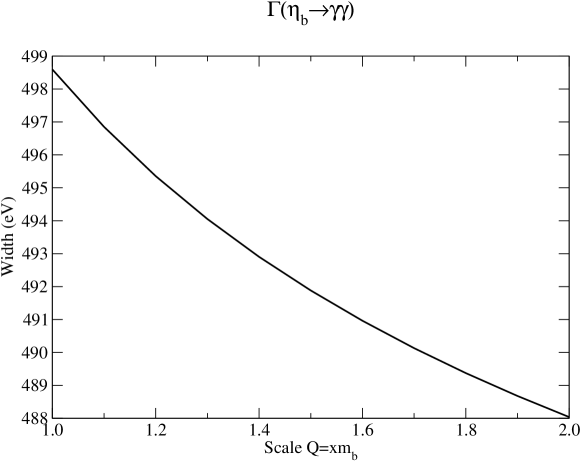
Figure 1: The dependence of the $\eta_{b}$ decay width to $\gamma\gamma$ (in eV) is shown with respect to the scale chosen for $\alpha_{s}$ in the radiative corrections.

Here we have assumed the $\alpha_{s}$ scale to be $Q=2m_{b}=10.0\textrm{ GeV}$. This choice is by no way unique as shown for the $\eta_{c}$ decay [3], and in fig. (1) we show the dependence of the $\eta_{b}$ photonic width, evaluated from eq. (4), upon different values of the scale chosen for $\alpha_{s}$ . Since there are no experimental measurements of this decay we shall assume, like for the $\eta_{c}$ case, that it is not possible to determinate a scale choice of $\alpha_{s}$ . We shall therefore include this fluctuation in the indetermination due to radiative corrections.

3 Potential models predictions for $\eta_{b}$

We present now the results one can obtain for the absolute width, through the extraction of the wave function at the origin from potential models. For the calculation of the wavefunction [15] we have used four different potential models, like the potential of Rosner et al. [4] $V(r)=\lambda((r/r_{0})^{\alpha}-1)/\alpha+C\mbox{ .}$ with $r_{0}=1\textrm{ GeV}^{-1},\;\alpha=-0.14\mbox{ , }\lambda=0.808\textrm{ GeV, }C=-1.305\textrm{ GeV}$, and the QCD inspired potential $V_{J}$ of Igi-Ono [5, 16]

$$V_{J}(r)=V_{AR}(r)+dre^{-gr}+ar,\ \ \ V_{AR}(r)=-\frac{4}{3}\frac{\alpha_{s}^{(2)}(r)}{r}$$ (6)

with two different parameter sets, corresponding to $\Lambda_{\overline{MS}}=0.5\ GeV$ and $\Lambda_{\overline{MS}}=0.2\ GeV$ respectively [5].

$\Lambda_{\overline{MS}}(GeV)$	$a(GeV^{2})$	$g(GeV)$	$d(GeV^{2})$
0.2	0.1587	0.3436	0.2550
0.5	0.1391	2.955	1.776

Table 1: Parameters chosen for Igi–Ono potential $V_{J}(r)$.

We also show the results from a Coulombic type potential with the QCD coupling $\alpha_{s}$ frozen to a value of $r$ which corresponds to the Bohr radius of the quarkonium system, $r_{B}=3/(2m_{b}\alpha_{s})$ (see for instance [6]). We shall stress that the scale of $\alpha_{s}$ occurring in the radiative correction and the one of Coulombic potential are different.

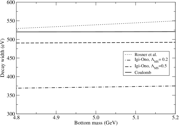
Figure 2: The dependence of $\eta_{b}$ decay width to $\gamma\gamma$ in eV for different potential models is shown as a function of $m_{b}$ .

We show in fig. (2) the predictions for the decay width from these potential models with the correction from eq. (1) at an $\alpha_{s}$ scale $Q=2m_{b}$ . For any given model, sources of error in this calculation arise from the choice of scale in the radiative correction factor and the choice of the parameters. Including the fluctuations of the results given by the different models, we can estimate a range of values for the potential model predictions for the radiative decay width $\Gamma(\eta_{b}\to\gamma\gamma)$, namely

$$\Gamma(\eta_{b}\to\gamma\gamma)=466\pm 101\textrm{ eV \mbox{ }.}$$ (7)

4 Octet component procedure

We will present now another approach which admits other components to the meson decay beyond the one from the colour singlet picture (Bodwin, Braaten and Lepage) [7]. NRQCD has been used to separate the short distance scale of annihilation from the nonperturbative contributions of long distance scale. This model has been successfully used to explain the larger than expected $J/\psi$ production at the Tevatron and LEP. According to BBL, in the octet model for quarkonium, the electromagnetic and light hadrons ($LH$) decay widths of bottomonium states are given by:

$$\Gamma(\Upsilon\to LH) = \frac{2\langle\Upsilon|O_{1}(^{3}S_{1})|\Upsilon\rangle}{m_{b}^{2}}\left(\frac{10}{243}\pi^{2}-\frac{10}{27}\right)\alpha_{s}^{3}\times\left[1+\left(-9.46\times\frac{4}{3}+\right.\right.$$

$$+12.39-1.161n_{f} \left.\left.\right)\frac{\alpha_{s}}{\pi}\right]+\frac{2\langle\Upsilon|P_{1}(^{3}S_{1})|\Upsilon\rangle}{m_{b}^{4}}\frac{17.32\times\left[20(\pi^{2}-9)\right]}{486}\alpha_{s}^{3}$$ (8)

$$\Gamma(\Upsilon\to e^{+}e^{-}) = \frac{2\langle\Upsilon|O_{1}(^{3}S_{1})|\Upsilon\rangle}{m_{b}^{2}}\left[\frac{\pi}{3}Q^{2}\alpha^{2}\left(1-\frac{13}{3}\frac{\alpha_{s}}{\pi}\right)\right]-$$ (9)

$$- \frac{2\langle\Upsilon|P_{1}(^{3}S_{1})|\Upsilon\rangle}{m_{b}^{4}}\frac{4}{9}\pi Q^{2}\alpha^{2}$$

$$\Gamma(\eta_{b}\to LH) = \frac{2\langle\eta_{b}|O_{1}(^{1}S_{0})|\eta_{b}\rangle}{m_{b}^{2}}\frac{2}{9}\pi\alpha_{s}^{2}\left[1+\left(\frac{53}{2}-\frac{31}{24}\pi^{2}-\frac{8}{9}n_{f}\right)\right]-$$ (10)

$$- \frac{2\langle\eta_{b}|P_{1}(^{1}S_{0})|\eta_{b}\rangle}{m_{b}^{4}}\frac{8}{27}\pi\alpha_{s}^{2}$$

$$\Gamma(\eta_{b}\to\gamma\gamma) = \frac{2\langle\eta_{b}|O_{1}(^{1}S_{0})|\eta_{b}\rangle}{m_{b}^{2}}\pi Q^{4}\alpha^{2}\left[1+\left(\frac{\pi^{2}-20}{3}\right)\frac{\alpha_{s}}{\pi}\right]-$$ (11)

$$- \frac{2\langle\eta_{b}|P_{1}(^{1}S_{0})|\eta_{b}\rangle}{m_{b}^{4}}\frac{4}{3}\pi Q^{4}\alpha^{2}$$

There are four unknown long distance coefficients, which can be reduced to two by means of the vacuum saturation approximation:

$$G_{1}\equiv\langle\Upsilon|O_{1}(^{3}S_{1})|\Upsilon\rangle=\langle\eta_{b}|O_{1}(^{1}S_{0})|\eta_{b}\rangle$$ (12)

$$F_{1}\equiv\langle\Upsilon|P_{1}(^{3}S_{1})|\Upsilon\rangle=\langle\eta_{b}|P_{1}(^{1}S_{0})|\eta_{b}\rangle$$ (13)

correct up to $\mathcal{O}(v^{2})$, where ${\vec{v}}$ is the quark velocity inside the meson. Since $v$ is of order $\alpha_{s}(M)$, there is no increase of accuracy if the matrix elements are calculated to order $v^{2}$ before coefficients are known to order beyond $\alpha_{s}$.

With this position we are able to use the $\Upsilon$ experimental decay widths as input in order to determine the long distance coefficients $G_{1}$ and $F_{1}$ . This result in turn is used to compute the $\eta_{b}$ decay widths.

The BBL procedure gives the following decay widths of the $\eta_{b}$ meson:

$$\Gamma(\eta_{b}\rightarrow\gamma\gamma)=364\pm 8\pm 13\textrm{ eV}$$ (14)

and

$$\Gamma(\eta_{b}\rightarrow LH)=57.9\pm 4.6\pm 2.8\textrm{ keV ,}$$ (15)

where the first error comes from the uncertainty on the $\Upsilon$ experimental width, the second error from $\alpha_{s}$ .

The improvement of the error on eq. (14) with respect to the previous analogous determination on the $\eta_{c}$ decay [3] is due to better error on the experimental measures of the $\Upsilon$ decay widths compared to the one of the $J/\psi$, and the smaller indetermination on the $\alpha_{s}$ value due to the higher energy scale involved in the decay. These reasons, together with the fact that the potential models used are fitted for the $c\overline{c}$ system, justifies the improvement of accuracy given in eq. (14) compared to the one of eq. (7).

5 Comparison between models

For comparison we present in fig. (3) a set of predictions coming from different methods. Starting with potential models, we see that the results are in good agreement with each other. The advantage of this method is that we are giving a prediction from first principles, without using any experimental input. Since there are currently no experimental measures for the $\eta_{b}\to\gamma\gamma$ decay, we shall use this prediction as a reference point, as it has proven to be reliable in the case of charmonium decay [3]. The second evaluation, given by BBL using the experimental values of the $\Upsilon$ decay, is on the left limit of the potential models value. This is true also for the determination of the BBL procedure with nonperturbative long distance terms taken from from the lattice calculation [17], affected from a large error. The advantage of the latter is that its prediction, like the one from potential models, does not make use of any experimental value. Next is the point given by the singlet picture from the electromagnetic decay of the $\Upsilon$, aligned with the aforementioned results of the BBL procedure. The point above is obtained also from the singlet picture with the $\Upsilon$ decay into light hadrons, in agreement with the results given from the potential models. We notice that in analogy to the charmonium case (see [3] and references therein) the singlet results obtained from the $\Upsilon$ decay are in disagreement with each other, in this case by only $1\sigma$. The last point from a two–loop enhanced calculation given by [8, 2] is in agreement with the potential model result and the singlet decay from the $\Upsilon\to LH$ process.

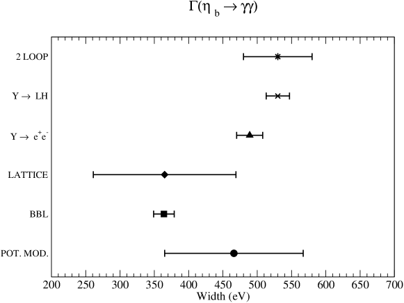
Figure 3: The $\eta_{b}$ two photon width as calculated in this paper using (starting from below) Potential Models results, BBL procedure with input from $J/\psi$ decay data, Lattice evaluation of $G_{1}$ and $F_{1}$ factors, Singlet picture with $G_{1}$ obtained from $\Upsilon\to e^{+}e^{-}$ and $\Upsilon\to LH$ processes respectively, and the two–loop enhanced procedure.

6 Conclusions

The $\Gamma(\eta_{b}\to\gamma\gamma)$ decay width prediction of the potential models considered gives the value $466\pm 101\textrm{ eV}$, in agreement with the naive estimate from the $\Upsilon$ decay given by (5). Predictions of the BBL procedure are consistent with the potential model results, for both the long distance terms $G_{1}$ and $F_{1}$ extracted from the $\Upsilon$ experimental decay widths and the one evaluated from lattice calculations. The results from the singlet picture are also consistent with the potential model results. Finally the two–loop enhanced prediction is in good agreement with the potential model results.

References

- [1] A. Böhrer, hep-ph/0110030, to appear in proceedings of “PHOTON 2001”, Ascona, Switzerland (2001), ed. by M. Kienzle, World Sci., Singapore, 2001, and private communication.
- [2] The ALEPH Collaboration, A. Heister et al., Phys. Lett. B 530 (2002) 56.
-
[3]
N. Fabiano, G. Pancheri, hep-ph/0110211,
to appear in proceedings of “PHOTON 2001”, Ascona, Switzerland
(2001), ed. by M. Kienzle, World Sci., Singapore, 2001;
N. Fabiano, G. Pancheri, hep-ph/0204214, to be published in Eur. Phys. J. C. - [4] A.K. Grant, J.L. Rosner and E. Rynes, Phys. Rev. D 47 (1993) 1981.
-
[5]
J. H. Kühn and S. Ono, Zeit. Phys. C21
(1984) 385;
K. Igi and S. Ono, Phys. Rev. D 33 (1986) 3349. - [6] N. Fabiano, A. Grau and G. Pancheri, Phys. Rev. D 50 (1994) 3173; Nuovo Cimento A, Vol 107 (1994) 2789.
- [7] G.T. Bodwin, E. Braaten and G.P. Lepage, Phys. Rev. D 51 (1995) 1125.
- [8] A. Czarnecki and K. Melnikov, Phys. Lett. B 519 (2001) 212.
- [9] R.Van Royen and V.Weisskopf, Nuovo Cimento 50A (1967) 617.
- [10] R. Barbieri, G. Curci, E. d’Emilio and R. Remiddi Nuclear Physics B154 (1979) 535.
- [11] P. Mackenzie and G. Lepage, Phys. Rev. Lett. 47 (1981) 1244.
- [12] E. Eichten, K. Gottfried, T. Kinoshita, K. D. Lane and T. M. Yan, Phys. Rev. 21D (1980) 203.
- [13] E. Eichten and F. Feinberg, Phys. Rev. D23, (1981) 2724.
- [14] Review of Particle Properties, D.E. Groom et al., Eur. Phys. J. C 15 (2000) 1; http://pdg.lbl.gov/.
-
[15]
Thanks to F.F. Schöbrl for providing the program;
W. Lucha, F.F. Schöbrl, Int. J. Mod. Phys. C 10 (1999) 607. - [16] W. Buchmuller and S. H. H. Tye, Phys. Rev. D24 (1981) 132.
- [17] G.T. Bodwin, D.K. Sinclair and S. Kim, Int. J. Mod. Phys. A 999 (2001) 123.