Abstract

We go beyond parameterizations of soft terms in superstring models and investigate the dynamical assumptions that lead to the relative strength of the dilaton vs the moduli contributions in the soft breaking. Specifically, we discuss in some simple heterotic orbifold models sufficient conditions to achieve dilaton dominance. Assuming self-dual points to be minima we find multiple solutions to the trilinear and bilinear soft parameters $A_{0}$ and $B_{0}$. We discuss the constraints on $\mu$ and $\tan\beta$ in superstring models in the context of radiative breaking of the electroweak symmetry. We show that string models prefer a small to a moderate value of $\tan\beta$, i.e. $\tan\beta\leq 10$, and a value much larger than this requires a high degree of fine tuning. Further, we show that for large $\tan\beta$ the radiative electroweak symmetry breaking constraint leads to a value $\alpha_{string}=g_{string}^{2}/4\pi$ which is typically an order of magnitude smaller than implied by the LEP data and the heterotic superstring relation $g_{string}=k_{i}g_{i}$, where $g_{i}$ is the gauge coupling constant for the gauge group ${\cal G}_{i}$ and $k_{i}$ is the corresponding Kac-Moody level in the class of models considered. This situation can be overcome by another fine tuned cancellation between the dilaton and the moduli contributions in the soft parameters.

One of the challenges facing string theory is to generate a unified model of interactions which includes in it the successes of the standard model. Many attempts have been made over the years in this direction. This includes model building within the heterotic string framework, i.e. models based on Calabi-Yau compactifications and orbifolds [1], and models based on M-theory and D-branes [2]. In this paper we examine soft breaking in some simple heterotic models, under the constraints of modular invariance ($T$-duality), and investigate the dynamical conditions that govern the relative strength of the dilaton and the moduli contribution to the soft parameters. We also discuss the constraints that relate $\mu$ and $\tan\beta$ in string theory in the context of radiative breaking of the electroweak symmetry.

The scalar potential in supergravity and string theory is given by [3, 4]

$$V=e^{d}[(d^{-1})^{i}_{j}D_{i}WD_{j}^{\dagger}W^{\dagger}-3WW^{\dagger}]+V_{D-term},$$ (1)

where $d$ is the Kähler potential, $W$ is superpotential and $D_{i}W=W_{i}+d_{i}W$, with the subscripts denoting derivatives w.r.t. to the corresponding fields. We will focus our attention on the heterotic superstring compactifications on orbifolds, although without going into their details. The only constraint that we want to use is the $T$-duality symmetry, from which we pick up a generic SL(2,Z) subgroup of modular invariance associated to large–small radius symmetry. Specifically, the scalar potential in the effective four dimensional theory depends on the dilaton field $S$ and on the (Kähler) moduli fields $T_{i}$, and it is invariant under the modular transformations

$$T_{i}\rightarrow T^{\prime}_{i}=\frac{a_{i}T_{i}-ib_{i}}{ic_{i}T_{i}+d_{i}},(a_{i}d_{i}-b_{i}c_{i})=1,~{}~{}~{}a_{i},b_{i},c_{i},d_{i}\in Z$$ (2)

Under the modular transformations, $d$ and $W$ undergo a Kähler transformation: $W{\rightarrow}We^{-f}$, $d\rightarrow d+f+\bar{f}$, $f=\sum_{i}log(ic_{i}T_{i}+d_{i})$ while the combination $G\equiv d+ln(WW^{\dagger})$ is invariant. Further, in general, if a function $f$ transforms under modular transformations as $f\rightarrow(ic_{i}T_{i}+d_{i})^{n_{1}}$ $(-ic_{i}\bar{T}+d_{i})^{n_{2}}f$ then it is assigned the weight $(n_{1},n_{2})$. The constraints of duality have proven useful in the investigation of gaugino condensation and SUSY breaking in previous analyses [5, 6]. In our analysis we will assume that $W$ is decomposable as $W=W_{h}+W_{v}$, where $W_{h}$ is the superpotential which depends only on the fields of the hidden sector and $W_{v}$ is the superpotential for the physical fields, i.e. quarks, leptons and Higgs fields. The origin of supersymmetry breaking in string theory is not yet fully understood. However, one conjectures that it originates in the hidden sector via gaugino condensation [7, 8]. We will not address this issue here but assume that stable minima exist and supersymmetry breaking can be achieved. We are interested in the nature of the soft terms that appear and the constraints on them from radiative breaking of the electroweak symmetry. We will discuss some specific models based on the generic form of the Kähler potential and of the superpotential. Thus for the Kähler potential we assume:

$$d=D-\sum_{i}log(T_{i}+\bar{T}_{i})+K_{IJ}Q_{I}^{\dagger}Q_{J}+H_{IJ}Q_{I}Q_{J},$$ (3)

where, as a model for $D$, one may consider $D=-ln(S+\bar{S}+\frac{1}{4\pi^{2}}\sum_{i}^{3}\delta_{i}^{GS}log(T_{i}+\bar{T}_{i}))$. Here, $\delta_{i}^{GS}$ is the one loop correction to the Kähler potential from the Green-Schwarz mechanism [9]. For the superpotential $W_{v}$ we assume a form $W_{v}=\tilde{\mu}_{IJ}Q_{I}Q_{J}+\lambda_{IJK}Q_{I}Q_{J}Q_{K}$, where $Q$ are the matter fields consisting of the quarks, leptons and the Higgs. Under $T$-duality, $Q$’s transform as $Q_{I}\rightarrow Q_{I}\Pi_{i}(ic_{i}T_{i}+d_{i})^{n^{i}_{Q_{I}}}$. In general, $K_{IJ},H_{IJ},\mu_{IJ}$ and $\lambda_{IJK}$ are functions of the moduli. The constraints on $n^{i}_{Q_{I}}$ are such that $G$ is modular invariant.

Soft breaking in string models has been studied by many authors. However, most of these analyses have been at the level of parameterizations of the breaking. We are interested in investigating more deeply the dynamical underpinnings of soft breaking in string models, specifically in determining the dynamical constraints needed to achieve dilaton dominance or admixtures of dilaton and moduli participation in the breaking. Further, modular invariance implies that the scalar potential is stationary at the self dual points. The exact nature of these stationary points depends on detailed dynamical considerations which do not address here and for the purpose of this analysis we assume that the self dual points are indeed minima. The conclusions of this analysis would be essentially unaffected if the true minima were not exactly at the self dual points. Our focus will be the Higgs sector of the theory since it is this sector that controls the electroweak symmetry breaking and much of the low energy physics of sparticles that will be hunted at the particle accelerators. To keep the analysis simple we impose the tree level condition $\delta^{GS}_{i}=0$. We also make the simplifying assumptions that $H_{IJ}=0$. These assumptions would not necessarily hold in a realistic string model but some of the lessons of the analysis may be helpful in string model building. Below we consider three models in their increasing level of complexity.

The first model we consider is where the set of moduli fields is limited to the dilaton $S$ and one overall modulus $T$. We consider a Kähler potential of the form

$$d=D(S,\bar{S})-3ln(T+\bar{T})+h_{1}^{\dagger}h_{1}+h_{2}^{\dagger}h_{2}+\sum_{\alpha\neq h_{1},h_{2}}(T+\bar{T})^{n_{c_{\alpha}}}C_{\alpha}^{\dagger}C_{\alpha}$$ (4)

where $h_{1,2}$ are the two higgs doublets of the minimal supersymmetric standard model (MSSM) with modular weights (0,0) and modular invariance implies that the remaining fields of MSSM obey the condition $n_{Q}+n_{U^{c}}=n_{Q}+n_{D^{c}}=n_{L}+n_{E^{c}}=-3$. One of the constraints on the scalar potential is that of the vanishing of the vacuum energy which in this case requires

$$|\gamma_{S}|^{2}+|\gamma_{T}|^{2}=1,~{}~{}|\gamma_{S}|^{2}\equiv-\frac{1}{3}\left.(d^{-1})^{S}_{\bar{S}}\frac{D_{S}WD_{\bar{S}}{W^{\dagger}}}{WW^{\dagger}}\right|_{0},~{}~{}|\gamma_{T}|^{2}\equiv-\frac{1}{3}\left.(d^{-1})^{T}_{\bar{T}}\frac{D_{T}WD_{\bar{T}}{W^{\dagger}}}{WW^{\dagger}}\right|_{0}$$ (5)

where the subscript 0 means that we are evaluating the quantities in the vacuum state. Now for the model of Eq.(4) we find $|\gamma_{T}|^{2}=\frac{(T+\bar{T})^{2}}{9}\frac{D_{T}W_{h}D_{\bar{T}}W^{\dagger}_{h}}{W_{h}W^{\dagger}_{h}}$, with $D_{T}W_{h}=\partial_{T}W_{h}-\frac{3W_{h}}{T+\bar{T}}$. We assume that the modular dependence of $W_{h}$ is of the form

$$W_{h}=\frac{F(S,T)}{\eta(T)^{6}},$$ (6)

where $\eta(T)$ is the Dedekind function and $F(S,T)$ is modular invariant, in general a function of the absolute modular invariant $j(T)$ [10]. Under this assumption, one finds

$$|\gamma_{T}|^{2}=(T+\bar{T})^{2}(G_{2}(T)-\frac{1}{3}D_{T}logF(S,T))(G_{2}(\bar{T})-\frac{1}{3}D_{\bar{T}}log\bar{F}(\bar{S},\bar{T}))$$ (7)

where $G_{2}(T)\equiv 2\partial_{T}ln\eta(T)+1/{(T+\bar{T})}$. The modular invariance of $|\gamma_{T}|^{2}$ is easily checked from the transformation properties of $\eta(T)$ and $\tilde{G}_{2}=G_{2}-\frac{1}{3}D_{T}logF(S,T)$, i.e. $\eta(T)\rightarrow(icT+d)^{1/2}\eta(T)$,   $\tilde{G}_{2}(S,T)\rightarrow(icT+d)^{2}$ $\tilde{G}_{2}(S,T)$. For MSSM, $W_{v}$ takes on the form $W_{v}=\mu h_{1}h_{2}$ + $\sum_{\alpha\beta\gamma}w_{\alpha\beta\gamma}$, where $w_{\alpha\beta\gamma}=\lambda_{\alpha\beta\gamma}C_{\alpha}C_{\beta}C_{\gamma}$ are the cubic interactions invariant under $SU(3)_{C}\times SU(2)_{L}\times U(1)_{Y}$ and $\lambda_{\alpha\beta\gamma}$ are the Yukawas. Following the usual technique of computation of soft terms [3, 11, 12, 13], one gets

$$V_{(Soft)}\!\! = m_{3/2}^{2}((h_{1}^{\dagger}h_{1}+h_{2}^{\dagger}h_{2})+\!\!\sum_{\alpha\neq h_{1},h_{2}}(T+\bar{T})^{n_{C_{\alpha}}}C_{\alpha}^{\dagger}C_{\alpha})+(B_{0}\mu h_{1}h_{2}+\sum_{\alpha\beta\gamma}A_{\alpha\beta\gamma}^{0}w_{\alpha\beta\gamma}+H.c.),$$

$$m_{3/2}^{2} = \langle e^{-G}\rangle=\langle\frac{e^{D}W_{h}W_{h}^{\dagger}}{(T+\bar{T})^{3}}\rangle,$$

$$A_{\alpha\beta\gamma}^{0} = \bar{m}(3|\gamma_{T}|^{2}-\sqrt{3}|\gamma_{S}|(1-(S+\bar{S})\partial_{S}ln\lambda_{\alpha\beta\gamma})e^{-i\theta_{s}}),$$

$$B_{0} = \bar{m}(-1+3|\gamma_{T}|^{2}-\sqrt{3}|\gamma_{S}|(1-(S+\bar{S})\partial_{S}ln\tilde{\mu})e^{-i\theta_{s}}),$$ (8)

with $(S+\bar{S})G_{,S}/\sqrt{3}=|\gamma_{S}|e^{i\theta_{s}}$, $\bar{m}=m_{3/2}\frac{e^{D/2-i\theta}}{(T+\bar{T})^{3/2}}$, and where $\langle W_{h}\rangle/|\langle W_{h}\rangle|=e^{i\theta}$. Noting that $W_{h}W_{h}^{\dagger}$ has modular weight (-3,-3) while $T+\bar{T}$ has modular weight (-1,-1), one finds that $m_{3/2}^{2}$ is modular invariant. Further, $\mu h_{1}h_{2}$ and $w_{\alpha\beta\gamma}$ in Eq.(8) have modular weight (-3,0) each while $A^{0}$ and $B_{0}$ have modular weights (3,0) each, and thus $V_{(Soft)}$ is explicitly modular invariant. We note that we cannot go to the canonical basis, where the kinetic energies of all the fields (including quarks and leptons) are normalized, at arbitrary points in the moduli space without destroying the holomorphicity of the superpotential. However, we can do so once the moduli are fixed, such as by going to the self dual points $T=1,e^{i\pi/6}$. where we assume the potential is minimized. Here $\bar{m}$ takes on the values $\bar{m}=m_{3/2}(\frac{e^{D/2-i\theta}}{2\sqrt{2}},\frac{e^{D/2-i\theta}}{3^{3/4}})$ for $T=(1,e^{i\pi/6})$. We distinguish now the following two cases: (i) $F$ has a non-trivial $T$-dependence: Here the vanishing of $G_{2}(T)$ at the self dual points gives $|\gamma_{T}|^{2}=\frac{1}{9}(T+\bar{T})^{2}D_{T}logF(S,T)D_{\bar{T}}log\bar{F}(\bar{S},\bar{T})$. In this case one has both dilaton and moduli participation in the soft breaking at the self dual points. (ii) $F$ has no dependence on $T$: Here the vanishing of $G_{2}(T)$ at the self dual points gives $\gamma_{T}=0$, $|\gamma_{S}|=1$, for $T=1,e^{i\pi/6}$ and leads to dilaton dominance of soft breaking at the self dual points. We normalize the quark and lepton fields and denote the normalized fields by lower case symbols, $c_{\alpha}=q,u^{c},d^{c},l,e^{c}$ and denote the Yukawas for the normalized fields by $Y_{\alpha\beta\gamma}$ so that $w_{\alpha\beta\gamma}=\lambda_{\alpha\beta\gamma}C_{\alpha}C_{\beta}C_{\gamma}$= $Y_{\alpha\beta\gamma}c_{\alpha}c_{\beta}c_{\gamma}$. Further, we limit ourselves to the case where $\mu$ and $Y_{\alpha\beta\gamma}$ have no dependence on the dilaton field so that $A_{0}=A_{\alpha\beta\gamma}^{0}$. Then $A_{0},B_{0}$ take on the following values at the self-dual points:

$$(A_{0},B_{0})=\left(\matrix{-\frac{\sqrt{3}}{2\sqrt{2}}m_{3/2}e^{D/2-i(\theta+\theta_{s})},~{}~{}\frac{e^{D/2-i\theta}}{2\sqrt{2}}m_{3/2}(-1-\sqrt{3}e^{-i\theta_{s}})\cr-\frac{1}{3^{1/4}}m_{3/2}e^{D/2-i(\theta+\theta_{s})},~{}~{}\frac{e^{D/2-i\theta}}{3^{3/4}}m_{3/2}(-1-\sqrt{3}e^{-i\theta_{s}})}\right)~{}~{}~{}\left(\matrix{T=1\cr T=e^{i\pi/6}}\right)$$ (9)

Next we consider a model where the Kähler potential is similar to that of Eq.(4), except that the Higgs fields also have modular weights. Thus we consider a Kähler potential of the following form

$$d=D(S,\bar{S})-3ln(T+\bar{T})+\sum_{\alpha}(T+\bar{T})^{n_{C_{\alpha}}}C_{\alpha}^{\dagger}C_{\alpha}$$ (10)

where the sum on $\alpha$ now runs over all the MSSM fields. The vanishing of the vacuum energy again gives Eq.(5) and a computation of the soft terms gives

$$V_{(Soft)}=m_{3/2}^{2}(\sum_{\alpha}(T+\bar{T})^{n_{C_{\alpha}}}C_{\alpha}^{\dagger}C_{\alpha})+(B_{0}\tilde{\mu}H_{1}H_{2}+\sum_{\alpha\beta\gamma}A_{\alpha\beta\gamma}^{0}w_{\alpha\beta\gamma}+H.c.)$$ (11)

where $m_{3/2}$, $A_{\alpha\beta\gamma}^{0},B_{0}$ are again easily computed as in the preceding case. The modular invariance of $V_{soft}$ is easily checked using $n_{Q}+n_{H_{2}}+n_{U^{c}}=-3$, $n_{Q}+n_{H_{1}}+n_{D^{c}}=-3$, $n_{L}+n_{H_{1}}+n_{e^{c}}=-3$. We again consider the case where $\mu$ and $\lambda_{\alpha\beta\gamma}$ have no dilaton dependence. As in the above example, we cannot normalize the fields at arbitrary points in the moduli space but can do so at the self dual points. Going to the basis where the fields are canonically normalized at the self dual points we can write $V_{(Soft)}$=$m_{3/2}^{2}(\sum_{\alpha}c_{\alpha}^{\dagger}c_{\alpha}$$)+$$(B_{0}W^{(2)}+A_{0}W^{(3)}+H.c.)$ where $W^{(2)}=\mu h_{1}h_{2}$, and $W^{(3)}$= $Y_{qh_{2}u^{c}}qh_{2}u^{c}$ + $Y_{qh_{1}d^{c}}qh_{1}d^{c}$ + $Y_{lh_{1}e^{c}}lh_{1}e^{c}$. Here $h_{1},h_{2},q,u^{c},d^{c},l,e^{c}$ are the normalized fields and the factors needed to normalize the fields have been absorbed in $\mu$, $Y_{qh_{2}u^{c}}$ etc so that $\mu=\tilde{\mu}/[(T+\bar{T})_{SD}^{n_{H_{1}}/2}(T+\bar{T})_{SD}^{n_{H_{2}}/2}]$ and $Y_{qh_{2}u^{c}}$ = $\lambda_{qh_{2}u^{c}}$ $/[(T+\bar{T})_{SD}^{n_{H_{2}}/2}$ $(T+\bar{T})_{SD}^{n_{Q}/2}$ $(T+\bar{T})_{SD}^{n_{U^{c}}/2}]$  etc.

Finally, we consider the model with many moduli. We take for our Kähler potential the form

$$d=D(S,\bar{S})-\sum_{i}ln(T_{i}+\bar{T}_{i})+\sum_{i\alpha}(T_{i}+\bar{T}_{i})^{n_{C_{\alpha}}^{i}}C_{\alpha}^{\dagger}C_{\alpha}$$ (12)

Here, for each $T_{i}$, the superpotential has modular weight -1 and one has $D_{T_{i}}(W)=\partial_{T_{i}}W-\frac{1}{T_{i}+\bar{T}_{i}}W$, and $D_{T_{i}}(W)=-\tilde{G}_{2}(S,T_{i})W$ for each i, where $\tilde{G}_{2}(S,T_{i})=G_{2}(T_{i})-D_{T_{i}}logF(S,T_{i})$. The condition for the vanishing of the vacuum energy in this case is $|\gamma_{S}|^{2}+\sum_{i}|\gamma_{i}|^{2}=1$ where $|\gamma_{i}|^{2}=-\frac{1}{3}(G^{-1})^{i}_{\bar{i}}G_{i}G_{\bar{i}}$. An analysis similar to the one before gives $|\gamma_{i}|^{2}$=$\frac{(T_{i}+\bar{T}_{i})^{2}}{3}$ $\tilde{G}_{2}(S,T_{i})$$\tilde{G}_{2}(\bar{S},\bar{T}_{i})$. We note that $|\gamma_{i}|^{2}$ has a relative factor of $1/3$ compared to $|\gamma_{T}|^{2}$. In this case,

$$V_{soft}=m_{3/2}^{2}(\sum_{i,\alpha}(T_{i}+\bar{T}_{i})^{n_{C_{\alpha}}^{i}}C_{\alpha}^{\dagger}C_{\alpha})+(B_{0}\tilde{\mu}H_{1}H_{2}+\sum_{\alpha\beta\gamma}A_{\alpha\beta\gamma}^{0}w_{\alpha\beta\gamma}+H.c.)$$

$$A_{\alpha\beta\gamma}^{0}=\bar{m}(3\sum_{i}|\gamma_{i}|^{2}-\sqrt{3}|\gamma_{S}|(1-(S+\bar{S})\partial_{S}ln\lambda_{\alpha\beta\gamma})e^{-i\theta_{s}}),$$

$$~{}B_{0}=\bar{m}(-1+3\sum_{i}|\gamma_{i}|^{2}-\sqrt{3}|\gamma_{S}|(1-(S+\bar{S})\partial_{S}ln\tilde{\mu})e^{-i\theta_{s}}),$$ (13)

with $\bar{m}=m_{3/2}{e^{D/2-i\theta}}/{\Pi_{i}(T_{i}+\bar{T}_{i})^{1/2}}$. In the overall modulus case $\sum_{i}|\gamma_{i}|^{2}=|\gamma_{T}|^{2}$ and the result of Eq.(8) can be obtained from Eq.(13) by setting $T_{1}=T_{2}=T_{3}=T$. We can go to the canonical basis as in previous cases. Further, since normalizing factors do not have a dilaton dependence we can replace $\lambda_{\alpha\beta\gamma}$ by $Y_{\alpha\beta\gamma}$ and replace $\tilde{\mu}$ by $\mu$ in Eq.(13). Thus at the self dual points $T_{i}=(1,e^{i\pi/6})$, and $A^{0}$ and $B_{0}$ of Eq.(13) reduce to

$$A_{\alpha\beta\gamma}^{0}=m_{3/2}e^{D/2-i\theta}(3\sum_{i}|\gamma_{i}|^{2}-\sqrt{3}|\gamma_{S}|(1-(S+\bar{S})\partial_{S}lnY_{\alpha\beta\gamma})e^{-i\theta_{s}})/f_{\alpha}^{\frac{1}{2}}$$

$$B_{0}=m_{3/2}e^{D/2-i\theta}(-1+3\sum_{i}|\gamma_{i}|^{2}-\sqrt{3}|\gamma_{S}|(1-(S+\bar{S})\partial_{S}ln\mu)e^{-i\theta_{s}})/f_{\alpha}^{\frac{1}{2}}$$ (14)

where $\{f_{\alpha}\}=8,4\sqrt{3},6,3\sqrt{3}$ and the multiplicity of $f_{\alpha}$ arises from the degeneracy of the allowed vacua. Again if $D_{T_{i}}F=0$, i.e. if $F$ has no $T_{i}$ dependence then $\gamma_{i}=0$ and soft breaking at the self dual points is dilaton-dominated. However, if $D_{T_{i}}F$ is non vanishing at the self dual point, then $\gamma_{i}$ are also non vanishing and moduli enter in soft breaking. In actual string calculations one does not encounter modular invariant $F$ functions which have nontrivial $T_{i}$ dependence. In this circumstance one has dilaton dominance in the class of models we are considering.

Although the $\mu$ term is supersymmetric and not a soft parameter, the origin of $\mu$ is most likely soft breaking. In fact, one common mechanism for its generation is in the Kähler potential where an $H_{1}H_{2}$ can arise with a dimensionless coefficient which can be naturally O(1). This term when transfered via a Kähler transformation to the superpotential gives a $\mu$ of the same size as the soft terms [14]. A concrete example of this mechanism in string theory was given in the analysis of Ref.[15] where it was shown that an $H_{1}H_{2}$ term does indeed arise in the Kähler potential. However, this computation was for the invariant $\bf 27\,\overline{27}$ involving a generation and an anti generation. Thus the result of Ref.[15] is not directly applicable to the case where the Higgs are both generational. The analysis of two-generational Higgs is more difficult since an invariant cannot be formed out of two 27’s. For the purpose of the present analysis we assume that a string computation following the technique of Ref.[15] can be extended to determine the $\mu$ term needed in MSSM. In addition to the above the soft breaking contains the gaugino masses which are given by

$$M_{\alpha}=\frac{1}{2}{Ref_{\alpha}}^{-1}e^{-G/2}f_{\alpha a}(G^{-1})^{a}_{b}G^{b},$$ (15)

where $f_{\alpha}$ is the gauge kinetic energy function and for a gauge group ${\cal G}=\Pi_{\alpha}{\cal G}_{\alpha}$, it is given by [16] $f_{\alpha}=k_{\alpha}S+\sum\frac{1}{4\pi^{2}}[C({\cal G}_{\alpha})-\sum_{I}T(R^{\alpha}_{Q_{I}})(1+2n^{i}_{Q_{I}})-2k_{\alpha}\delta^{GS}_{i}]log(\eta(T_{i}))+\dots,$ where $k_{\alpha}$ is the Kac-Moody level for the subgroup ${\cal G}_{\alpha}$. In our investigation below it would suffice to consider just the tree contribution which yields a universal gaugino mass $m_{1/2}$ for the simplest case of $k_{\alpha}=1$. In this case one has

$$m_{1/2}=\sqrt{3}m_{3/2}|\gamma_{S}|e^{-i\theta_{s}}$$ (16)

Under the assumption that $D_{T}F(S,T)=0$ and when one is at the self dual points, $\gamma_{i}=0$, $|\gamma_{S}|=1$ and one has the result for the gaugino masses in the dilaton dominance case.

Radiative electroweak symmetry breaking imposes important constraints on string model building. However, before discussing the constraint of radiative breaking in string theory let us review the situation in supergravity models first. In the minimal supergravity grand unified models one starts out with five parameters $m_{0},m_{1/2},A_{0},B_{0},\mu$ at the GUT scale [3, 12]. The renormalization group effects in running the SUSY parameters with the GUT boundary conditions to the low scale allow the $H_{2}$ Higgs mass to turn tachyonic, due to its couplings to the top quark, which triggers the breaking of the electroweak symmetry. One of the conditions for the minimization of the potential ${\partial V_{H}}/{\partial v_{i}}=0$ yields [17]

$$\mu^{2}=-\frac{1}{2}M_{Z}^{2}+\frac{m_{h_{1}}^{2}-m_{h_{2}}^{2}\tan^{2}\beta}{\tan^{2}\beta-1}$$ (17)

where $m^{2}_{h_{i}}$ ($i=1,2$) contain the one-loop corrections from the effective potential [18] and $\tan\beta\equiv\langle h_{2}\rangle/\langle h_{1}\rangle$. In supergravity models $\mu$ is a free parameter and thus one uses the radiative symmetry breaking constraint to determine $\mu$ from Eq.(17) (see e.g. Ref.[19]). We discuss now the situation in string theory where $\mu$ is determined in principle (for recent papers on phenomenology under the constraints of modular invariance see Refs.[20, 21, 22]). On the other hand the radiative symmetry breaking equation also determines $\mu$. How can these two determinations, one from string theory and the other from radiative breaking of the electroweak symmetry breaking, be reconciled? Clearly once the string determined values of $m_{h_{1}},m_{h_{2}}$ and $\mu$ are used in the radiative symmetry breaking constraint Eq.(17) and since $M_{Z}$ is determined from experiment, the only thing left to determine is $\tan\beta$ and so we write Eq.(17) in the form

$$\tan^{2}\beta=\frac{\mu^{2}+\frac{1}{2}M_{Z}^{2}+m_{h_{1}}^{2}}{\mu^{2}+\frac{1}{2}M_{Z}^{2}+m_{h_{2}}^{2}}$$ (18)

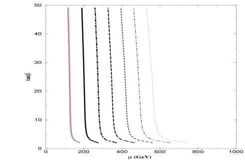
Figure 1: Exhibition of the fine tuning problem in string models at large tanbeta. The curves are for the scenario with dilaton dominance of soft breaking when $m_{3/2}$ takes on the values $50,75,100,125,150,175,200$ all masses in GeV. The Higgs mass parameters at the unification scale are universal so that $m_{h_{1}}(0)=m_{3/2}=m_{h_{2}}(0)$.

Eq.(18) imposes a stringent constraint on string models. Specifically we show below that Eq.(18) implies that large $\tan\beta$, i.e. $\tan\beta>10$ is disfavored in string models as such values require a high degree of fine tuning. This fine tuning is different from the one encountered in supergravity models where $\mu$ can be used to define the fine tuning [23]. In the numerical analysis below we assume no dilaton dependence of $\mu$ and $Y_{\alpha\beta\gamma}$. In Fig.1 we give a plot of $\tan\beta$ vs $\mu$ for the scenario with dilaton dominance of soft breaking. For the large $\tan\beta$ case $A_{0}$ nearly vanishes as will be discussed in the context of Fig.2 and so we have set $A_{0}=0$ in the analysis of Fig.1 (our conclusions, however, derived from Fig.1 are largely independent of the value of $A_{0}$). We notice the sharp rise in $\tan\beta$ for values of $\tan\beta$ greater than in the range 5-10. For values of $\tan\beta$ above this range the slope as a function of $\mu$ becomes very large. This region thus corresponds to the region of high fine tuning. This means that if we want values of $\tan\beta$ greater than 5-10 we will have to fine tune our moduli with extreme accuracy. Further, we note that this fine tuning appears to be a generic feature of string models independent of the details of the soft terms. The origin of this fine tuning is easily understood since a large $\tan\beta$ can only arise when the denominator in Eq.(18) nearly vanishes. In the vicinity of the point where the denominator nearly vanishes the sensitivity to small changes is magnified. Thus consider as a measure of sensitivity the quantity $f_{i}$ defined by $f_{i}=|\frac{1}{\tan\beta}\frac{\partial\tan\beta}{\partial t_{i}}|$ where $t_{i}$ are the moduli on which $\tan\beta$ depends. Using Eq.(18) one finds that $f_{i}\propto\tan^{2}\beta$. Thus $|\frac{\partial\tan\beta}{\partial t_{i}}|\propto\tan^{3}\beta$ and for large $\tan\beta$ this behavior leads to a high degree of fine tuning to achieve a large value of $\tan\beta$ as is seen in Fig.1. Thus we conclude that in string models large $\tan\beta$ is problematic, requiring a large degree of fine tuning of the moduli.

The constraints of radiative electroweak symmetry in string models are even more severe than discussed above. Thus the second electroweak symmetry breaking condition can be written in the form

$$\sin 2\beta=\frac{-2\mu B}{m_{h_{1}}^{2}+m_{h_{2}}^{2}+2\mu^{2}}$$ (19)

where all parameters are evaluated at the electroweak scale. Since the quantities in Eq.(19) are all determined in string theory, Eq.(19) becomes a constraint on the moduli themselves. We illustrate this constraint for the large $\tan\beta$ case. We note that $\sin 2\beta$ nearly vanishes for the case of large $\tan\beta$ and from Eq.(19) we deduce that $B$ must nearly vanish for the case of large $\tan\beta$. From Eqs.(8) and (14) we find that this can happen either if there is a large exponential suppression of several e-folds arising from the factor $e^{D/2}$ or if there is a cancellation between the dilaton and the moduli contributions which requires a fine tuning. We will see that in most of the parameter space of the moduli the cancellation does not provide a sufficient suppression and one needs an exponential suppression from the dilaton factor $e^{D/2}$. The same exponential suppression also suppresses $A_{0}$. Now $D$ is related to the string coupling constant

$$e^{-D}=\frac{2}{g_{string}^{2}}$$ (20)

where $g_{string}=k_{i}g_{i}$ and $k_{i}$ is the Kac-Moody level of the gauge group ${\cal G}_{i}$ and $g_{i}$ is the corresponding gauge coupling constant. Eq.(20), upon using the value of $D$ implied by Eq.(19), allows one to compute $\alpha_{string}$ at the unification scale $M_{X}$ in terms of the parameters at the electroweak scale. Thus for the model of Eq.(14), setting $\theta=\theta_{s}=0$, one gets

$$\alpha_{string}=\frac{1}{2\pi}\frac{(\mu^{2}+\frac{1}{2}M_{Z}^{2}+m_{h_{1}}^{2})^{2}}{\mu^{2}m_{3/2}^{2}r_{B}^{2}(1+\epsilon_{Z})^{2}\tan^{2}\beta}\frac{f_{\alpha}}{(-1+3\sum_{i}|\gamma_{i}|^{2}-\sqrt{3}|\gamma_{S}|(1-(S+\bar{S})\partial_{S}ln\mu))^{2}}$$ (21)

where $\epsilon_{Z}=M_{Z}^{2}/(m_{h_{1}}^{2}+\mu^{2}-\frac{1}{2}M_{Z}^{2}+(m_{h_{1}}^{2}+\mu^{2}+\frac{1}{2}M_{Z}^{2})\cot^{2}\beta)$ and $r_{B}$ is the renormalization group coefficient that relates $B_{0}$ at the unification scale $M_{X}$ to $B$ at the electroweak scale, i.e. $B=r_{B}B_{0}$. In Fig.2 we give a plot of $\alpha_{string}(M_{X})$ at the unification scale as a function of $\tan\beta$ for the dilaton dominance case (i.e., $\sum_{i}|\gamma_{i}|^{2}=0$) where we assume no dilaton dependence of $\mu$ and $Y_{\alpha\beta\gamma}$.. One finds that for large $\tan\beta$ the value of $\alpha_{string}(M_{X})$ is far too small to be consistent with the LEP constraints on $\alpha_{string}(M_{X})$ necessary for unification of gauge coupling constants. In Fig.3 we give a plot of $\alpha_{string}$ as a function of $\gamma_{S}$ for the case $\tan\beta=50$. One finds that $\alpha_{string}$ is typically small for much of the range of $\gamma_{S}$ except for a small element where the denominator in Eq.(21) passes through a zero. We note that compatibility with LEP data in this case can occur only over a minuscule range at two points where the horizontal curve intersects the vertical lines because of the rapid slope of the curves there. Further agreement with LEP date requires a significant cancellation between the dilaton and the moduli contributions in the denominator in Eq.(21). In the above we assumed $k_{i}=1$. For the Kac-Moody levels $k_{i}>1$ the situation is even worse. Thus we conclude that on the basis of the fine tuning problem and the problem of too small a value of $\alpha_{string}$ encountered for the case of large $\tan\beta$ that large $\tan\beta$ values are not preferred in string models of the type we are considering. There are important implications of this constraint for accelerator and dark matter experiments. Thus, for example, the decay $B^{0}_{s}\rightarrow\l^{+}l^{-}$ which requires a large $\tan\beta$ to become visible within the sensitivities that would be achievable at RUNII of the Tevatron [25] would not have a chance of being seen in string models unless fine tuning is invoked. Similarly, detection rates for the direct detection of dark matter depend strongly on $\tan\beta$ and increase with increasing $\tan\beta$ and thus a small $\tan\beta$ value would make the search for dark matter more difficult. On the plus side a smaller $\tan\beta$ leads to a longer proton life time in supersymmetric unified theories and is thus preferable from the point of view of proton stability [26]. The current experimental data from LEP and from the Tevatron only put mild lower limit constraints on $\tan\beta$ which are consistent with the constraints on $\tan\beta$ from strings. Similarly, the recent data from Brookhaven [27] on g-2 gives a difference between experiment and theory of about $1.6\sigma$ to $2.6\sigma$. Such a difference can be understood within string models of the type discussed above with a value of $\tan\beta$ below 10 [28].

In conclusion, we have investigated soft breaking in string models under the constraints of modular invariance and additional simplifying assumptions to understand more clearly the relationship of the dilaton and the moduli in soft breaking. In our analysis we found sufficient dynamical constraints that allow for dilaton dominance of soft breaking at the self dual points. In our analysis we assumed that the minima are at the self-dual points. However, the constraints of modular invariance require only that the self dual points be either minima, maxima or saddle points, and do not exclude existence of other stationary points. If the minima were away from the self dual points, the values of $f_{\alpha}$ would be somewhat different. However, if they lie close to the self dual points, as in Ref.[29], the modifications of $f_{\alpha}$ would be small. Thus while the above results were derived within some model examples, it appears likely that they may be valid for a larger class of string models.

This work is supported in part by NSF grant PHY-9901057. T.R.T. is grateful to Dieter Lüst and the Institute of Physics at Humboldt University in Berlin for their kind hospitality during completion of this work. We thank Thomas Dent for bringing to our attention Ref.[29].

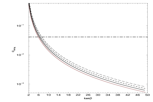
Figure 2: Exhibition of $\alpha_{string}$ evaluated at the unification scale as a function of $\tan\beta$ for the scenario with dilaton dominance of soft breaking when $m_{3/2}=150$ GeV for the case of Eq.(14) of model 3. The Higgs mass parameters at the unification scale are universal so that $m_{h_{1}}(0)=m_{3/2}=m_{h_{2}}(0)$ and $A_{0}=0$ as in Fig.1. The four curves in descending order correspond to the four degenerate vacua at the self dual points corresponding to $f_{\alpha}=8$, $4\sqrt{3}$, $6$, $3\sqrt{3}$. The horizontal line is the value of $\alpha_{string}$ at the unification scale needed for consistency with the LEP data.

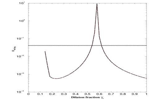
Figure 3: Exhibition of $\alpha_{string}$ evaluated at the unification scale as a function of the dilaton fraction $\gamma_{S}$ when $m_{3/2}=150$ GeV for the case of Eq.(14) of model 3 with $\tan\beta=50$ and $f_{\alpha}=6$. Gaugino masses are given by Eq.(16) and the Higgs masses are $m_{3/2}$ at the unification scale and $A_{0}=0$ as in Fig.1. All phases are set to zero. The horizontal line is as in Fig.2.

References

- [1] For a sample of heterotic string models see, L.E.Ibanez, H. P. Nilles and F. Quevedo, Nucl. Phys. B307 (1988) 109; A. Antoniadis, J.Ellis, J. Hagelin, and D.V. Nanopoulos, Phys. Lett. B194 (1987) 231; B. R. Green, K. H. Kirklin, P.J. Miron G.G. Ross, Nucl. Phys.B292 (1987) 606; R. Arnowitt and P. Nath, Phys. Rev. D40 (1989) 191; A. H. Chamseddine and M. Quiros, Nucl. Phys. B 316 (1989) 101; D.C. Lewellen, Nucl. Phys. B337 (1990) 61; A. Farragi, Phys. Lett. B278 (1992) 131; S. Chaudhuri, S.-W. Chung, G. Hockney, and J.D. Lykken, Nucl. Phys.452 (1995) 89; G.B. Cleaver, Nucl. Phys. B456 (1995) 219; M. Cvetic and P. Langacker, Phys. Rev. D54 (1996) 3570; Z. Kakushadze and S.H.H. Tye, Phys. Rev. D55 (1997) 7896; ibid, D56 (1997) 7878; Phys. Lett. 392 (1997) 325.
- [2] G. Aldazabal, L. E. Ibanez and F. Quevedo, JHEP 0001 (2000) 031; G. Aldazabal, L. E. Ibanez, F. Quevedo and A. M. Uranga, JHEP 0008 (2000) 002; M. Cvetic, G. Shiu and A. M. Uranga, Nucl. Phys. B 615 (2001) 3; M. Cvetic, G. Shiu and A. M. Uranga, Phys. Rev. Lett. 87 (2001) 201801; D. Bailin, G. V. Kraniotis and A. Love, arXiv:hep-th/0208103; C. Kokorelis, JHEP 0209, 029 (2002).
- [3] A. H. Chamseddine, R. Arnowitt and P. Nath, Phys. Rev. Lett. 49 (1982) 970; P. Nath, R. Arnowitt and A.H. Chamseddine, “Applied N=1 Supergravity”, World Scientific, 1984
- [4] E. Cremmer, S. Ferrara, L. Girardello and A. Van Proeyen, Nucl. Phys. B 212 (1983) 413.
- [5] S. Ferrara, N. Magnoli, T. R. Taylor and G. Veneziano, Phys. Lett. B 245 (1990) 409; A. Font, L. E. Ibanez, D. Lüst and F. Quevedo, Phys. Lett. B 245 (1990) 401; H. P. Nilles and M. Olechowski, Phys. Lett. B 248 (1990) 268; P. Binetruy and M. K. Gaillard, Phys. Lett. B 253 (1991) 119; M. Cvetic, A. Font, L. E. Ibanez, D. Lüst and F. Quevedo, Nucl. Phys. B 361 (1991) 194.
- [6] A. Brignole, L. E. Ibanez, C. Munoz and C. Scheich, Z. Phys. C 74 (1997) 157; B. de Carlos, J. A. Casas and C. Munoz, Nucl. Phys. B 399 (1993) 623; A. Brignole, L. E. Ibanez and C. Munoz, Phys. Lett. B 387 (1996) 769.
- [7] H. P. Nilles, Phys. Lett. B 115 (1982) 193; S. Ferrara, L. Girardello and H. P. Nilles, Phys. Lett. B 125 (1983) 457; M. Dine, R. Rohm, N. Seiberg and E. Witten, Phys. Lett. B 156 (1985) 55; C. Kounnas and M. Porrati, Phys. Lett. B 191 (1987) 91.
- [8] T. R. Taylor, Phys. Lett. B 252 (1990) 59; D. Lüst and T. R. Taylor, Phys. Lett. B 253 (1991) 335.
- [9] G. Lopes Cardoso and B. A. Ovrut, Nucl. Phys. B 369 (1992) 351; J. P. Derendinger, S. Ferrara, C. Kounnas and F. Zwirner, Nucl. Phys. B 372 (1992) 145; I. Antoniadis, E. Gava, K. S. Narain and T. R. Taylor, Nucl. Phys. B 407 (1993) 706;
- [10] K. Chandrasekharan, Elliptic Functions (Berlin: Springer Verlag, 1985). See also B. R. Greene, A. D. Shapere, C. Vafa and S. T. Yau, Nucl. Phys. B 337 (1990) 1.
- [11] R. Barbieri, S. Ferrara and C. A. Savoy, Phys. Lett. B 119 (1982) 343.
- [12] L. J. Hall, J. Lykken and S. Weinberg, Phys. Rev. D 27 (1983) 2359; P. Nath, R. Arnowitt and A. H. Chamseddine, Nucl. Phys. B 227 (1983) 121.
- [13] L. E. Ibanez and D. Lüst, Nucl. Phys. B 382 (1992) 305; V. S. Kaplunovsky and J. Louis, Phys. Lett. B 306 (1993) 269.
- [14] G. F. Giudice and A. Masiero, Phys. Lett. B 206 (1988) 480.
- [15] I. Antoniadis, E. Gava, K. S. Narain and T. R. Taylor, Nucl. Phys. B 432 (1994) 187.
- [16] V. S. Kaplunovsky, Nucl. Phys. B 307 (1988) 145; L. J. Dixon, V. Kaplunovsky and J. Louis, Nucl. Phys. B 355 (1991) 649; I. Antoniadis, K. S. Narain and T. R. Taylor, Phys. Lett. B 267 (1991) 37; P. Mayr and S. Stieberger, Nucl. Phys. B 407 (1993) 725; B 412 (1994) 502; Phys. Lett. B 355 (1995) 107; G. Lopes Cardoso, D. Lüst and T. Mohaupt, Nucl. Phys. B 450 (1995) 115.
- [17] L. Alvarez-Gaume, J. Polchinski and M. B. Wise, Nucl. Phys. B 221 (1983) 495.
- [18] S. R. Coleman and E. Weinberg, Phys. Rev. D 7 (1973) 1888; R. Arnowitt and P. Nath, Phys. Rev. D 46 (1992) 3981.
- [19] R. Arnowitt and P. Nath, Phys. Rev. Lett. 69 (1992) 725.
- [20] P. Binetruy, M. K. Gaillard and B. D. Nelson, Nucl. Phys. B 604 (2001) 32; M. K. Gaillard, B. D. Nelson and Y. Y. Wu, Phys. Lett. B 459 (1999) 549; M. K. Gaillard and J. Giedt, Nucl. Phys. B 636 (2002) 365.
- [21] G. Kane, J. Lykken, B. Nelson and L. T. Wang, hep-ph/0207168; G. Kane, J. Lykken, S. Mrenna, Brent D. Nelson, L.-T. Wang, T. T. Wang, hep-ph/0209061
- [22] T. Dent, JHEP 0112 (2001) 028 [arXiv:hep-th/0111024]; arXiv:hep-ph/0208164;
- [23] K. L. Chan, U. Chattopadhyay and P. Nath, Phys. Rev. D 58 (1998) 096004.
- [24] K. R. Dienes, Phys. Rept. 287 (1997) 447.
- [25] See, e.g., T. Ibrahim and P. Nath, arXiv:hep-ph/0208142 and the references therein.
- [26] J. R. Ellis, D. V. Nanopoulos and S. Rudaz, Nucl. Phys. B 202 (1982) 43; P. Nath, A. H. Chamseddine and R. Arnowitt, Phys. Rev. D 32 (1985) 2348; J. Hisano, H. Murayama and T. Yanagida, Nucl. Phys. B 402 (1993) 46.
- [27] G. W. Bennett [Muon g-2 Collaboration], arXiv:hep-ex/0208001.
- [28] U. Chattopadhyay and P. Nath, (to appear in Phys. Rev. D), arXiv:hep-ph/0208012.
- [29] D. Bailin, G. V. Kraniotis and A. Love, Phys. Lett. B 435, 323 (1998)