Resummation of nuclear enhanced higher twist in the Drell Yan process

Abstract

We investigate higher twist contributions to the transverse momentum broadening of Drell Yan pairs in proton nucleus collisions. We revisit the contribution of matrix elements of twist-4 and generalize this to matrix elements of arbitrary twist. An estimate of the maximal nuclear broadening effect is derived. A model for nuclear enhanced matrix elements of arbitrary twist allows us to give the result of a resummation of all twists in closed form. Subleading corrections to the maximal broadening are discussed qualitatively.

I Introduction

In the era of RHIC and LHC the understanding of hard processes in heavy ion collisions plays an increasingly important role. It has become clear that the onset of the regime of perturbative quantum chromodynamics (pQCD) with increasing momentum transfer in reactions involving large nuclei can be very different from that in collisions of single hadrons. Previous studies have shown that the leading twist approximation CSS:mueller in pQCD, even at intermediate momentum transfers, can be spoiled by higher components of the twist expansion.

The reason for that is that matrix elements of higher twist can be increasingly sensitive to the size of the nucleus. With naive power counting, twist-2 parton distributions scale with the mass number $A$ of the nucleus, while matrix elements of twist-$(2m+2)$, $m\in\mathbb{N}$, can scale with $m$ additional powers of $A^{1/3}$. These matrix elements are then called nuclear enhanced. They correspond to processes with multiple scattering. For large nuclei these additional factors of $A^{1/3}$ can compensate the inherent power suppression of higher twist.

Let us explore the physical picture RJF:hir behind this for the example of $p+A$ collisions. In the leading twist approximation only one parton $a$ from the nucleus and one parton $b$ from the proton participate in the hard scattering $a+b$. They are described by parton distributions respectively. A nuclear enhanced twist-4 matrix element for the nucleus corresponds to two partons $a$ and $a^{\prime}$ entering the hard scattering, They enable us to describe the process where the parton from the proton scatters off these two partons: $a\,a^{\prime}+b$. The additional factor of $A^{1/3}$ arises when the two partons come from different nucleons inside the nucleus. This mechanism was first pointed out by Luo, Qiu and Sterman some years ago LQS:92 ; LQS:94sv ; LQS:94 based on generalized factorization theorems QS:91 .

In the following years various calculations on the level of nuclear enhanced twist-4 (double scattering) became available for the Drell Yan process $p+A\to l^{+}l^{-}$ in proton nucleus collisions Guo:98ht ; FSSM:99 ; FSSM:00 . However going beyond the level of twist-4 remained a technically difficult point. It is known that for the Drell Yan process in symmetric colliding systems the QCD factorization fails at the level of twist-6 DFT . However in $p+A$ we will formally work in the limit of very large $A$ and therefore stay in the leading twist approximation for the proton. This allows us to go to arbitrary nuclear enhanced twist for the nucleus Qiu:hpc . Nevertheless a systematic calculation of contributions of arbitrary twist was never done in this framework.

In this publication we study the transverse spectrum of Drell Yan pairs and its nuclear broadening. This was already done on the level of twist-4 Guo:98jb . We will repeat this calculation both in light cone and covariant gauge for the strong interaction. In particular we comment on the question of electromagnetic gauge invariance. After that we generalize the result by calculating the contributions of operators of arbitrary twist. This is feasible for contributions which lead to maximal broadening, therefore establishing an upper bound on the nuclear effects on the transverse momentum spectrum. Besides this there are subleading contributions which we will also discuss shortly. We then present some arguments how the higher twist matrix elements can be approximated by model descriptions in such a way that we are able to give a closed expression for the sum of all higher twist contributions.

II Nuclear enhanced double scattering

In this section we will go through the calculation of the twist-4 contribution to the nuclear enhanced Drell Yan process. This computation was already done in covariant gauge by X. Guo some time ago Guo:98jb . We confirm her results. We also present an explicit calculation in light cone gauge, which bears some difficulties for higher twist. We also comment on the problem of electromagnetic gauge invariance in this calculation.

II.1 Light cone gauge

The Drell Yan cross section, integrated over the angular distribution and the rapidity of the lepton pair, is

$$\frac{d{\sigma}}{d{Q^{2}}d{q_{\perp}^{2}}}=\sum_{a}\frac{c_{a}^{2}\alpha}{24\pi^{2}SQ^{2}}\int dyP^{\mu\nu}W_{\mu\nu},$$ (1)

where $Q$, $q_{\perp}$ and $y$ are mass, transverse momentum and rapidity of the virtual photon and $S=(P_{1}+P_{2})^{2}$. $P_{1}$ and $P_{2}$ denote the four momenta of the nucleus (per nucleon) and the proton in the center of mass frame respectively. The sum runs over all quark flavors $a$ and $c_{a}$ is the charge of a given quark flavour relative to the electron charge. The hadronic tensor is defined as the matrix element of two electromagnetic currents

$$W_{\mu\nu}=\int d^{4}{y}e^{iq\cdot y}\left\langle P_{1}P_{2}\right|j^{\mu}(0)j^{\nu}(y)\left|P_{1}P_{2}\right\rangle$$ (2)

in the colliding system. After integrating the angular distribution the tensor $P^{\mu\nu}$ reduces to the polarization tensor of the virtual photon

$$P^{\mu\nu}=-g^{\mu\nu}+\frac{q^{\mu}q^{\nu}}{Q^{2}}$$ (3)

where $q$ is the four momentum of the virtual photon FSSM:00 . Electromagnetic gauge invariance of course requires that $q^{\mu}W_{\mu\nu}=0=W_{\mu\nu}q^{\nu}$.

We want to calculate the nuclear enhanced twist-4 contribution to the hadronic tensor. Thence we have to take into account the diagrams shown in Fig. 1. We denote the momenta of the quarks with $r_{1}$ and $r_{2}$ and the momenta of the gluons with $K$ and $K^{\prime}$. We expand the momenta of the parton lines between the hard and the soft part into a longitudinal contribution on the light cone and a transverse contribution

$$r_{1}^{\mu} =\xi_{1}P_{1}^{\mu}+r_{1}^{\perp} r_{2}^{\mu} =\xi_{2}P_{2}^{\mu}+r_{2}^{\perp}$$ (4)

$$K^{\mu} =xP_{1}^{\mu}+K^{\perp\mu} K^{\prime\mu} =x^{\prime}P_{1}^{\prime\mu}+K^{\prime\perp\mu}$$ (5)

introducing parton momentum fractions $x$, $x^{\prime}$, $\xi_{1}$ and $\xi_{2}$.

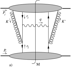
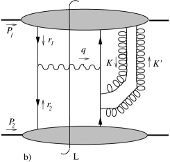
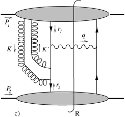
Figure 1: The diagrams contributing to Drell Yan on the level of twist-4. The symmetric diagram (a) is double scattering, the asymmetric diagrams (b) and (c) correspond to an interference of single and triple scattering.

The hadronic tensor for the symmetric diagram (a) is

$$W_{\mu\nu}^{(a)}=\frac{4\pi\alpha_{s}}{2N_{c}^{2}}\int d{y}\int\frac{d{\xi_{1}}}{\xi_{1}}\frac{d{\xi_{2}}}{\xi_{2}}\int P_{1}^{+}d{x}P_{1}^{+}d{x^{\prime}}{d^{2}}{r_{1}^{\perp}}{d^{2}}{K^{\perp}}{d^{2}}{K^{\prime\perp}}f_{\bar{q}}(\xi_{2})(32\pi^{3})\Gamma^{(a)}H^{(a)}_{\mu\nu,\rho\sigma}\frac{1}{(r_{2}+K)^{2}+i\epsilon}\\ \times\frac{1}{(r_{2}+K^{\prime})^{2}-i\epsilon}\int\frac{d{y_{1}^{-}}{d^{2}}{y_{1}^{\perp}}}{(2\pi)^{3}}\frac{d{y_{3}^{-}}{d^{2}}{y_{3}^{\perp}}}{(2\pi)^{3}}\frac{d{y_{4}^{-}}{d^{2}}{y_{4}^{\perp}}}{(2\pi)^{3}}e^{-i\xi_{1}P_{1}^{+}y_{1}^{-}}e^{-ixP_{1}^{+}y_{3}^{-}}e^{ix^{\prime}P_{1}^{+}y_{4}^{-}}e^{-ir_{1}^{\perp}\cdot y_{1}^{\perp}}e^{-iK^{\perp}\cdot y_{3}^{\perp}}e^{iK_{1}^{\prime\perp}\cdot y_{4}^{\perp}}\\ \frac{1}{2}\left\langle P_{1}\right|\bar{q}(0)\gamma^{+}q(y_{1}^{-},y_{1}^{\perp})A^{\rho}(y_{3}^{-},y_{3}^{\perp})A^{\sigma}(y_{4}^{-},y_{4}^{\perp})\left|P_{1}\right\rangle$$ (6)

for the case that the quark comes from the nucleus and the antiquark comes from the nucleon. Here

$$\Gamma^{(a)}=\delta[Q^{2}-(\xi_{1}+x)\xi_{2}S-(r_{1}^{\perp}+K^{\perp})^{2}]\\ \times\delta[q_{\perp}^{2}+(r_{1}^{\perp}+K^{\perp})^{2}]\delta\left[y-\frac{1}{2}\ln\frac{\xi_{1}+x}{\xi_{2}}\right]$$ (7)

are the momentum conserving $\delta$-functions which connect the photon momentum to the internal momenta. It is understood that the $\delta$-functions have to be integrated in order to obtain physical results. We have chosen to integrate the rapidity dependence of the cross section which is trivially done by the last $\delta$-function. The first $\delta$-function will be eliminated by the integral over $\xi_{2}$. At a later stage we will also integrate over ${q_{\perp}^{2}}$ but since we will do that in different ways it is a matter of convenience to keep the unphysical $\delta$-function in the mean time. $f_{\bar{q}}$ in above formula is the antiquark distribution in the proton.

The hard part $\cal{H}$ of the cross section is given by the propagators in Eq. (6), the phase factor $\Gamma^{(a)}$ and the trace

$$H^{(a)}_{\mu\nu,\rho\sigma}=\frac{1}{4}\operatorname{Tr}[\gamma_{\nu}(-r/\hskip 1.29167pt_{2}-K/\hskip 3.01385pt^{\prime})\gamma_{\sigma}r/\hskip 1.29167pt_{2}\gamma_{\rho}(-r/\hskip 1.29167pt_{2}-K/\hskip 3.01385pt)\gamma_{\mu}r/\hskip 1.29167pt_{1}].$$ (8)

The quark lines connecting the hard part to the nucleus and the nucleon respectively are contracted with $r/\hskip 1.29167pt_{1}$ and $r/\hskip 1.29167pt_{2}$ respectively. In order to project out the correct twist contribution there is an important step. We have to perform a collinear expansion of all momenta entering the hard part which is equivalent to a Taylor expansion in all transverse momenta. In light cone gauge for the gluon field we can stick to the 0th order of the expansion, i.e. we simply set all transverse momenta equal to zero. In Eq. (6) this was already done for the quark lines from the nucleon since we only wanted to generate the ordinary twist-2 parton distribution $f_{\bar{q}}(\xi_{2})$. For parton lines from the nucleus we keep the transverse momenta for the moment. The reason is that this collinear limit is not straightforward in light cone gauge. In fact, it will turn out that some contributions which are falsely taken to vanish in the collinear limit in light cone gauge give finite results because the zeros in the hard part are canceled by poles elsewhere.

The two remaining diagrams (b) and (c) in Fig. 1 have the same decomposition of the hadronic tensor but with denominators of the propagators replaced by

$$\frac{1}{(r_{2}+K^{\prime}-K)^{2}-i\epsilon}\>\frac{1}{(r_{2}+K^{\prime})^{2}-i\epsilon}\>,$$ (9)

$$\frac{1}{(r_{2}+K-K^{\prime})^{2}+i\epsilon}\>\frac{1}{(r_{2}+K)^{2}+i\epsilon}$$ (10)

for diagrams (b), (c) respectively, $\delta$-functions

$$\Gamma^{(b)}=\delta[Q^{2}-\xi_{1}\xi_{2}S-{r_{1}^{\perp}}^{2}]\\ \times\delta[q_{\perp}^{2}+{r_{1}^{\perp}}^{2}]\delta\left[y-\frac{1}{2}\ln\frac{\xi_{1}}{\xi_{2}}\right],$$ (11)

$$\Gamma^{(c)}=\delta[Q^{2}-(\xi_{1}+x-x^{\prime})\xi_{2}S\\[5.0pt] -(r_{1}^{\perp}+K^{\perp}-K^{\prime\perp})^{2}]\delta[q_{\perp}^{2}+(r_{1}^{\perp}+K^{\perp}-K^{\prime\perp})^{2}]\\[5.0pt] \times\delta\left[y-\frac{1}{2}\ln\frac{\xi_{1}+x-x^{\prime}}{\xi_{2}}\right]$$ (12)

and traces

$$H^{(b)}_{\mu\nu,\rho\sigma} =\frac{1}{4}\operatorname{Tr}[\gamma_{\nu}(-r/\hskip 1.29167pt_{2}-K/\hskip 3.01385pt^{\prime}+K/\hskip 1.29167pt)\gamma_{\rho}$$ (13)

$$\qquad\times(-r/\hskip 1.29167pt_{2}-K/\hskip 3.01385pt^{\prime})\gamma_{\sigma}r/\hskip 1.29167pt_{2}\gamma_{\mu}r/\hskip 1.29167pt_{1}],$$

$$H^{(c)}_{\mu\nu,\rho\sigma} =\frac{1}{4}\operatorname{Tr}[\gamma_{\nu}r/\hskip 1.29167pt_{2}(-r/\hskip 1.29167pt_{2}-K/\hskip 3.01385pt)\gamma_{\rho}$$ (14)

$$\qquad\times(-r/\hskip 1.29167pt_{2}-K/\hskip 3.01385pt+K/\hskip 3.01385pt^{\prime})\gamma_{\sigma}\gamma_{\mu}r/\hskip 1.29167pt_{1}].$$

Next we want to convert the gluon gauge fields to field strengths. In light cone gauge $A^{+}=0$ the transverse components of the $A$ fields give the dominant contribution and we can use

$$P_{1}^{+}A^{\rho}P_{1}^{+}A^{\sigma}=\frac{1}{ix}(\partial^{+}A^{\rho})\frac{1}{-ix^{\prime}}(\partial^{+}A^{\sigma})\\ \approx\frac{1}{xx^{\prime}}F^{+\omega}F_{\omega}^{\phantom{\omega}+}\left(-g_{\perp}^{\rho\sigma}/2\right)$$ (15)

By the introduction of the field strength tensors we make the poles in the parton momentum fractions $x$ and $x^{\prime}$ explicit that were hidden in the gluon gauge fields. It will turn out that these poles are artificial and will be canceled by zeros which are hidden in the hard part. This is a special feature of the calculation in light cone gauge.

We carry out the collinear expansion as the lowest order Taylor expansion of the hard part in the transverse momenta $r_{1}^{\perp}$, $K^{\perp}$ and $K^{\prime\perp}$

$${\cal H}(\perp)={\cal H}(\perp)\big{|}_{\perp=0}+\sum_{\perp}\perp\frac{\partial}{\partial\perp}{\cal H}(\perp)\big{|}_{\perp=0}+{\cal O}(\perp).$$ (16)

Here $\perp$ shortly stands for all the transverse momenta. Now we are able to carry out all transverse integrals and to eliminate all dependences on transverse coordinates in Eq. (6) in a trivial way. For diagram (a) this gives us

$$W_{\mu\nu}^{(a)}=\frac{32\pi^{3}\alpha_{s}}{N_{c}^{2}}\int d{y}\int\frac{d{\xi_{1}}}{\xi_{1}}\frac{d{\xi_{2}}}{\xi_{2}}\int d{x}d{x^{\prime}}f_{\bar{q}}(\xi_{2})\frac{1}{xx^{\prime}}\left[{\cal H}(r_{1}^{\perp},K^{\perp},K^{\prime\perp})\right]_{\perp\rightarrow 0}\left(-g_{\perp}^{\rho\sigma}/2\right)\\ \int\frac{d{y_{1}^{-}}}{2\pi}\frac{d{y_{3}^{-}}}{2\pi}d{y_{4}^{-}}e^{-i\xi_{1}P_{1}^{+}y_{1}^{-}}e^{-ixP_{1}^{+}y_{3}^{-}}e^{ix^{\prime}P_{1}^{+}y_{4}^{-}}\frac{1}{2}\left\langle P_{1}\right|\bar{q}(0)\gamma^{+}q(y_{1}^{-})F^{+\omega}(y_{3}^{-})F_{\omega}^{\phantom{\omega}+}(y_{4}^{-})\left|P_{1}\right\rangle.$$ (17)

Due to the subtle interplay of poles and zeros in light cone gauge we evaluate the hard part with transverse momenta however keeping in mind to take the limit ${\perp\rightarrow 0}$ at the end. There are some caveats. E.g. if we want to test electromagnetic gauge invariance it is clear that we must not take $q^{\mu}\lim_{\perp\rightarrow 0}W_{\mu\nu}$ but we must take $\lim_{\perp\rightarrow 0}q^{\mu}W_{\mu\nu}$ since the hadronic tensor contains $\delta$-functions which give $q^{\mu}$ a finite transverse component as long as the internal transverse momenta are still finite.

The denominators of the propagators can be transformed into poles in $x$ and $x^{\prime}$ via

$$\frac{1}{(r_{2}+K)^{2}+i\epsilon}\>\frac{1}{(r_{2}+K^{\prime})^{2}-i\epsilon}\\ =(\xi_{2}S)^{-2}\frac{1}{x+\frac{{K^{\perp}}^{2}}{\xi_{2}S}+i\epsilon}\>\frac{1}{x^{\prime}+\frac{{K^{\prime\perp}}^{2}}{\xi_{2}S}-i\epsilon}.$$ (18)

We define the prefactor and the tensor structure from the field strength into the trace and finally evaluate

$$H^{(a)}_{\mu\nu}=(\xi_{2}S)^{-2}H^{(a)}_{\mu\nu,\rho\sigma}\left(-g_{\perp}^{\rho\sigma}/2\right)\\ =\frac{\xi_{1}}{\xi_{2}S}\Big{[}2xx^{\prime}P_{1\>\mu}P_{1\>\nu}+xP_{1\>\mu}K^{\prime\perp}_{\nu}+x^{\prime}P_{1\>\nu}K^{\perp}_{\mu}\\ +\frac{1}{2}(K^{\perp\>\mu}K^{\prime\perp\>\nu}-K^{\perp\>\nu}K^{\prime\perp\>\mu})+\frac{1}{2}K^{\perp}\cdot K^{\prime\perp}g_{\mu\nu}\\ -\frac{K^{\perp}\cdot K^{\prime\perp}}{S}(P_{1\>\mu}P_{2\>\nu}+P_{2\>\mu}P_{1\>\nu})\Big{]}.$$ (19)

At this stage we see that the naive limit $\perp\rightarrow 0$ carries most of the terms in above equation to zero. However if we look at it more carefully through the factor $1/xx^{\prime}$ from the gluon fields we will encounter a $0/0$ situation which we have to resolve in order to obtain finite results.

For diagrams (b), (c) we get similar poles and the traces reduce to

$$H^{(b)}_{\mu\nu}=(\xi_{2}S)^{-2}H^{(b)}_{\mu\nu,\rho\sigma}\left(-g_{\perp}^{\rho\sigma}/2\right)\\ =\frac{x^{\prime}\xi_{1}}{\xi_{2}S}\Big{[}P_{1\>\nu}(K^{\prime\perp}-K^{\perp})_{\mu}\\ +\xi_{2}(P_{1\>\mu}P_{2\>\nu}+P_{2\>\mu}P_{1\>\nu})-\frac{1}{2}\xi_{2}Sg_{\mu\nu}\Big{]}\>,$$ (20)

$$H^{(c)}_{\mu\nu}=(\xi_{2}S)^{-2}H^{(c)}_{\mu\nu,\rho\sigma}\left(-g_{\perp}^{\rho\sigma}/2\right)\\ =\frac{x\xi_{1}}{\xi_{2}S}\Big{[}P_{1\>\mu}(K^{\perp}-K^{\prime\perp})_{\nu}\\ +\xi_{2}(P_{1\>\mu}P_{2\>\nu}+P_{2\>\mu}P_{1\>\nu})-\frac{1}{2}\xi_{2}Sg_{\mu\nu}\Big{]}$$ (21)

We carry out the integrals in $x$ and $x^{\prime}$ by taking the residues given by the poles from the propagators. By the usual trick we have to take into account the exponential factors in the matrix element to argue in which way to close the integration contour and thereby we introduce an ordering of the light cone coordinates by

$$\Theta^{(a)} = \Theta(y_{1}^{-}-y_{3}^{-})\Theta(-y_{4}^{-})\>,$$ (22)

$$\Theta^{(b)} = \Theta(-y_{3}^{-})\Theta(y_{3}^{-}-y_{4}^{-})\>,$$ (23)

$$\Theta^{(c)} = \Theta(y_{1}^{-}-y_{4}^{-})\Theta(y_{4}^{-}-y_{3}^{-})$$ (24)

for diagrams (a), (b) and (c) respectively.

At this stage we see that the limits $r_{1}^{\perp},{r^{\prime}}_{1}^{\perp}\rightarrow 0$, are trivial in the sense that there are no poles or zeros appearing by taking this limit. We can therefore set these transverse momenta to zero. This implies $K^{\prime\perp}=K^{\perp}$ and $x^{\prime}=x=-{K^{\perp}}^{2}/\xi_{2}S$. Now we add up the contributions of all three graphs. Note that the pole integrations introduce minus signs for graphs (2) and (3):

$$\Theta^{(a)}H^{(a)}_{\mu\nu}\Gamma^{(1)}-\Theta^{(b)}H^{(b)}_{\mu\nu}\Gamma^{(2)}-\Theta^{(c)}H^{(c)}_{\mu\nu}\Gamma^{(3)}=\\ \quad=\frac{x\xi_{1}}{\xi_{2}S}\Big{[}2xP_{1\mu}P_{1\nu}+(P_{1\mu}K_{\nu}^{\perp}+P_{1\nu}K_{\mu}^{\perp})\Big{]}\Theta^{(a)}\Gamma^{(a)}\\ \qquad-\frac{x\xi_{1}}{S}\big{[}\frac{1}{2}Sg_{\mu\nu}-P_{1\mu}P_{2\nu}-P_{1\nu}P_{2\mu}\big{]}\Theta^{(a)}\big{[}\Gamma^{(a)}-\Gamma^{(b)}]\big{]}\\ -\frac{x\xi_{1}}{S}\big{[}\frac{1}{2}Sg_{\mu\nu}-P_{1\mu}P_{2\nu}-P_{1\nu}P_{2\mu}\big{]}\Gamma^{(b)}\big{[}\Theta^{(a)}-\Theta^{(b)}-\Theta^{(c)}\big{]}.$$ (25)

Let us now discuss electromagnetic gauge invariance. After taking the poles all quark lines attaching to an arbitrary quark photon vertex in either diagram are on the mass shell. Therefore electromagnetic gauge invariance at this stage is ensured for each diagram separately by simple equations of motion. Let us denote the three terms on the three different lines on the right hand side of Eq. (25) by A, B and C starting from above. It is easy to check that C is separately gauge invariant and so is the sum of A and B. B and A alone are not gauge invariant as the contraction of A with $q^{\mu}$ gives $1/2\>x\xi_{1}K_{\perp}^{\nu}\Theta^{(a)}\Gamma^{(a)}$ which is then canceled by the same term with different sign originating from contraction of $q^{\mu}$ with B. As already discussed the $\delta$-functions determine $q^{\mu}=(\xi_{1}+x)P_{1}^{\mu}+\xi_{2}P_{2}^{\mu}+K^{\perp\mu}$ (for $\Gamma^{(a)}$) and $q^{\mu}=\xi_{1}P_{1}^{\mu}+\xi_{2}P_{2}^{\mu}$ (for $\Gamma^{(b)}$).

We will now drop the term C because the term $\Theta^{(a)}-\Theta^{(b)}-\Theta^{(c)}$ requires the partons from the nucleus to be bound together and leads to a twist-4 contribution which is not nuclear enhanced Guo:98ht ; FSSM:00 . The remaining term A+B is only proportional to $\Theta^{(a)}$ and is manifestly gauge invariant. We absorb $\Theta^{(a)}$ into the matrix element

$$T_{qg}(\xi_{1},x)=\int\frac{d{y_{1}^{-}}}{2\pi}\frac{d{y_{3}^{-}}}{2\pi}d{y_{4}^{-}}e^{-i\xi_{1}P_{1}^{+}y_{1}^{-}}e^{-ixP_{1}^{+}(y_{3}^{-}-y_{4}^{-})}\Theta^{(a)}\frac{1}{2}\left\langle P_{1}\right|\bar{q}(0)\gamma^{+}q(y_{1}^{-})F^{+\omega}(y_{3}^{-})F_{\omega}^{\phantom{\omega}+}(y_{4}^{-})\left|P_{1}\right\rangle.$$ (26)

We can write the hadronic tensor after summing over all diagrams and integrating over $\xi_{1}$ and $y$ as

$$W_{\mu\nu}=\frac{128\pi^{5}\alpha_{s}}{N_{c}^{2}}\int_{B}^{1}\frac{d{\xi_{2}}}{\xi_{2}}f_{\bar{q}}(\xi_{2})\lim_{K^{\perp}\rightarrow 0}T_{qg}(\xi_{1},x)H_{\mu\nu}$$ (27)

where $B=Q^{2}/S$, $\xi_{1}=Q^{2}/(\xi_{2}S)$ and

$$H_{\mu\nu}=\Big{[}2P_{1\mu}P_{1\nu}+\frac{1}{x}(P_{1\mu}K_{\nu}^{\perp}+P_{1\nu}K_{\mu}^{\perp})\Big{]}\frac{\delta(q_{\perp}^{2}-k_{\perp}^{2})}{(\xi_{2}S)^{2}}\\ -\big{[}\frac{1}{2}Sg_{\mu\nu}-P_{1\mu}P_{2\nu}-P_{1\nu}P_{2\mu}\big{]}\\ \times\frac{\big{[}\delta(q_{\perp}^{2}-k_{\perp}^{2})-\delta(q_{\perp}^{2})\big{]}}{x\xi_{2}S^{2}}.$$ (28)

We have introduced $k_{\perp}^{2}=-{K^{\perp}}^{2}\geq 0$.

We note that this expression still has poles due to our choice of gauge for the gluon fields, but as checked above electromagnetic gauge invariance is manifest. It is once more interesting to note that the term in above equation which is proportional to the transverse gluon momentum is needed to ensure gauge invariance for the entire hadronic tensor. This now justifies the careful treatment of the collinear limit.

We are ready to contract the hadronic tensor with the photon polarization tensor. Since $q^{\mu}H_{\mu\nu}$ is zero this is simply a contraction with $-g^{\mu\nu}$. The result is simple and finally allows to take the limit $K^{\perp}\to 0$ unambiguously, leading to

$$H_{\mu\nu}P^{\mu\nu}=\lim_{k_{\perp}^{2}\rightarrow 0}\frac{1}{k_{\perp}^{2}}\big{[}\delta(q_{\perp}^{2}-k_{\perp}^{2})-\delta(q_{\perp}^{2})\big{]}=-\delta^{\prime}(q_{\perp}^{2})\,.$$ (29)

The final result for the cross section is

$$\frac{d\sigma_{1}}{dQ^{2}dq_{\perp}^{2}}=\sum_{q}\frac{4\pi c_{q}^{2}\alpha^{2}}{3N_{c}Q^{2}S}\\ \times\int_{B}^{1}\frac{d\xi_{2}}{\xi_{2}}T_{qg}(\xi_{1})f_{\bar{q}}(\xi_{2})\left[-\frac{4\pi^{2}\alpha_{s}}{N_{c}}\delta^{\prime}(q_{\perp}^{2})\right]$$ (30)

with the known soft hard matrix element $T_{qg}(\xi_{1})=T_{qg}(\xi_{1},x=0)$. A second term proportional to $T_{\bar{q}g}f_{q}$ has to be added but is not explicitly shown. This indeed coincides with the result in Guo:98jb . We introduced a subscript “1” with the cross section to indicate that this is the contribution with one pair of gluon fields in the matrix element.

II.2 Covariant gauge

Let us briefly go through the corresponding calculation in covariant gauge, since this will be the technique we use later for arbitrary twist. We can again start from Eq. (6) and proceed along the same way as before, keeping transverse momenta for the gluon fields. However in covariant gauge we use

$$P_{1}^{+}A^{\rho}P_{1}^{+}A^{\sigma}\approx P_{1}^{\rho}A^{+}P_{1}^{\sigma}A^{+}.$$ (31)

We therefore define

$$H_{\mu\nu}^{(i)}=(\xi_{2}S)^{-2}P_{1}^{\rho}P_{1}^{\sigma}H_{\mu\nu,\rho\sigma}^{(i)},$$ (32)

where $H_{\mu\nu,\rho\sigma}^{(i)}$ are the traces for the graphs $i=a$, $b$ and $c$. In covariant gauge we have to carry out the collinear expansion to the second order in transverse momentum, applying the operator

$$\frac{1}{2!}K_{\lambda}^{\perp}K_{\kappa}^{\perp}\frac{d^{2}}{dK_{\lambda}^{\perp}dK_{\kappa}^{\perp}}\Big{|}_{K^{\perp}\to 0}$$ (33)

to the hard part. The explicit factors of transverse momentum are used to obtain field strength tensors in the matrix element via

$$K^{\perp}_{\lambda}A^{+}(y_{3})K^{\perp}_{\kappa}A^{+}(y_{4})\\ \approx F^{+\omega}(y_{3})F_{\omega}^{\phantom{\omega}+}(y_{4})\left(-g^{\perp}_{\lambda\kappa}/2\right).$$ (34)

After performing the pole integrations in $x$ and $x^{\prime}$ and integrating over $\xi_{1}$ and $y$ the hadronic tensor for diagram (a) is

$$W_{\mu\nu}^{(a)}=\frac{128\pi^{5}\alpha_{s}}{N_{c}^{2}}\int\frac{d\xi_{2}}{\xi_{2}}f_{\bar{q}}(\xi_{2})\frac{1}{\xi_{1}}\left(-\frac{g^{\perp}_{\lambda\kappa}}{2}\right)\\ \frac{1}{2!}\frac{d^{2}}{dK^{\perp}_{\lambda}dK^{\perp}_{\kappa}}\Big{|}_{K^{\perp}\to 0}T_{qg}(\xi_{1},x)\,{H}_{\mu\nu}^{(a)}\,\delta(q_{\perp}^{2}+K^{\perp 2})$$ (35)

where now $x=x^{\prime}=k_{\perp}^{2}/\xi_{2}S$ and $\xi_{1}=Q^{2}/\xi_{2}S$. Since

$$-g^{\mu\nu}H_{\mu\nu}^{(a)}=\xi_{1}\xi_{2}S,$$ (36)

the derivatives can only act on the transverse $\delta$-function and the phases in the matrix element.

For diagrams (b) and (c) Eq. (35) holds with an additional “$-$” sign and modified $\Theta$-functions $\Theta^{(b)}$ and $\Theta^{(c)}$. Furthermore the transverse $\delta$-function is just $\delta(q_{\perp}^{2})$ and $-g^{\mu\nu}H_{\mu\nu}^{(b)}=-g^{\mu\nu}H_{\mu\nu}^{(c)}=\xi_{1}\xi_{2}S$. Therefore from the asymmetric diagrams (b) and (c) we can only get nuclear enhanced contributions with derivatives on the phases in the matrix element. When we sum over all diagrams the terms with derivatives on phases are again proportional to

$$\Theta^{(a}-\Theta^{(b)}-\Theta^{(c)}\to 0$$ (37)

and therefore show no nuclear enhancement — confer the discussion below Eq. (25). We conclude that the only nuclear enhanced contribution can arise from the transverse $\delta$-function of the symmetric diagram. We have

$$\left(-\frac{g^{\perp}_{\lambda\kappa}}{2}\right)\frac{1}{2!}\frac{d^{2}}{dK^{\perp}_{\lambda}dK^{\perp}_{\kappa}}\Big{|}_{K^{\perp}\to 0}\delta(q_{\perp}^{2}+{K^{\perp}}^{2})\\ =-\delta^{\prime}(q_{\perp}^{2}).$$ (38)

This implies

$$\frac{d\sigma_{1}}{dQ^{2}dq_{\perp}^{2}}=\frac{4\pi c_{q}^{2}\alpha^{2}}{3N_{c}Q^{2}S}\\ \times\int_{B}^{1}\frac{d\xi_{2}}{\xi_{2}}T_{qg}(\xi_{1})f_{\bar{q}}(\xi_{2})\left[-\frac{4\pi^{2}\alpha_{s}}{N_{c}}\delta^{\prime}(q_{\perp}^{2})\right].$$ (39)

which coincides with the result in light cone gauge.

Let us shortly discuss the result of the twist-4 calculation. $\delta$-functions and their derivatives, strictly speaking, are only defined when they are integrated. This applies also to our result. We have to integrate over the transverse momentum in order to obtain an observable quantity. Let us define moments $Q_{\perp}^{2m}$ of the transverse momentum spectrum by

$$Q_{\perp}^{2m}=\int_{0}^{\infty}dq_{\perp}^{2}\>q_{\perp}^{2m}\frac{d\sigma}{dQ^{2}dq_{\perp}^{2}}.$$ (40)

We recall the leading twist result for the cross section in leading order in $\alpha_{s}$

$$\frac{d\sigma_{0}}{dQ^{2}dq_{\perp}^{2}}=\frac{4\pi c_{q}^{2}\alpha^{2}}{3N_{c}Q^{2}S}\int_{B}^{1}\frac{d\xi_{2}}{\xi_{2}}f_{q}(\xi_{1})f_{\bar{q}}(\xi_{2})\delta(q_{\perp}^{2}).$$ (41)

A simple integration over $q_{\perp}^{2}$ gives zero which implies that there is no nuclear enhanced twist-4 contribution from these graphs to the spectrum integrated over the transverse momentum

$$(Q_{\perp}^{0})_{1}=\frac{d\sigma_{1}}{dQ^{2}}=0.$$ (42)

The subscript “1” on the left hand side refers to the contribution from $\sigma_{1}$. This is in disagreement with the results of QZ . However, when we look at the second moment of the transverse momentum spectrum, we get a nuclear enhanced twist-4 contribution Guo:98jb

$$(Q_{\perp}^{2})_{1}=\frac{4\pi c_{q}^{2}\alpha^{2}}{3N_{c}Q^{2}S}\int_{B}^{1}\frac{d\xi_{2}}{\xi_{2}}T_{qg}(\xi_{1})f_{\bar{q}}(\xi_{2})\frac{4\pi^{2}\alpha_{s}}{N_{c}}.$$ (43)

From leading twist we obtain

$$(Q_{\perp}^{0})_{0} =\frac{4\pi c_{q}^{2}\alpha^{2}}{3N_{c}Q^{2}S}\int_{B}^{1}\frac{d\xi_{2}}{\xi_{2}}f_{q}(\xi_{1})f_{\bar{q}}(\xi_{2}),$$ (44)

$$(Q_{\perp}^{2})_{0} =0$$ (45)

for the first two moments. All higher moments vanish both for twist-2 and twist-4.

The soft-hard matrix element is usually approximated by

$$T_{qg}(\xi_{1})\approx\lambda^{2}A^{4/3}f_{q}(\xi_{1})$$ (46)

where $f_{q}$ is the nuclear parton distribution for a quark normalized to one nucleon and $\lambda^{2}=0.01$ GeV² Guo:98ht ; Guo:98jb ; FSSM:00 . This leads to an additional broadening of the transverse momentum spectrum in $p+A$ collisions compared to $p+p$ collisions

$$\Delta\langle q_{\perp}^{2}\rangle=\frac{[Q_{\perp}^{2}]_{pA}}{[Q_{\perp}^{0}]_{pA}}-\frac{[Q_{\perp}^{2}]_{pp}}{[Q_{\perp}^{0}]_{pp}}.$$ (47)

To twist-4 accuracy we have $Q_{\perp}^{2m}=(Q_{\perp}^{2m})_{0}+(Q_{\perp}^{2m})_{1}$. Using the model for the soft-hard matrix element we obtain Guo:98jb

$$\Delta\langle q_{\perp}^{2}\rangle=\frac{4\pi^{2}\alpha_{s}}{N_{c}}\lambda^{2}A^{1/3}.$$ (48)

The transverse momentum broadening with the characteristic $A^{1/3}$ scaling was observed by the Fermilab E772 collaboration McGMP:99 .

III Beyond double scattering

III.1 Preliminaries

The result of the last section raises the question whether terms of even higher twist contribute to higher moments of the transverse momentum spectrum. This is indeed the case and will eventually allow us to resum the contributions of different twist. To start we want to pin down what we are looking for. We are interested in contributions of Twist-$(2n+2)$, $n\in\mathbb{N}$, with maximal nuclear enhancement $A^{n/3}$. Therefore we take into account operators with $n$ pairs of soft gluons, each single pair a color singlet with no flow of momentum between these pairs. These are necessary conditions to achieve maximal nuclear enhancement. The diagram in Fig. 2 is an example with $2n$ gluons. Furthermore we use the argument, that in a large $N_{c}$ expansion the leading contribution is coming from planar diagrams tHo:74 . In order to handle the large number of possibilities to group $2n$ gluons together to pairs we stick to the leading order in $1/N_{c}$ and only take into account planar diagrams, i.e. with no gluon lines intersecting each other. See Fig. 3 for an example

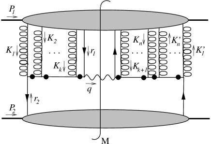
Figure 2: Scattering off 2n gluons. In this example $k$ gluons ($k<2n$) are on the left side and $2n-k$ gluons on the right side of the cut. The gluons are ordered to pairs with momenta $K_{i}$ and $K_{i}^{\prime}$ for one pair. Big dots indicate soft gluon poles.

We have seen that the case of twist-4 was simpler to handle in covariant gauge. Therefore we will use this gauge here. This requires us to take a derivative of the hard part of order $2n$ with respect to the transverse momenta. We denote the gluon momenta with $K_{1}$, $K_{2}$, … and $K^{\prime}_{1}$, $K^{\prime}_{2}$, …, where always $K_{i}$ and $K^{\prime}_{i}$ belong to one pair. We introduce parton momentum fractions by

$$K_{i}=x_{i}P_{1}+K^{\perp}_{i},\qquad K_{i}^{\prime}=x_{i}^{\prime}P_{1}+K^{\prime\perp}_{i}.$$ (49)

The differential operator we have to apply is of the form

$$\frac{1}{(2n)!}\prod_{i}K_{i}^{\perp\lambda_{i}}K_{i}^{\prime\perp\kappa_{i}}\frac{d^{2n}}{\prod_{i}dK_{i}^{\perp\lambda_{i}}dK_{i}^{\prime\perp\kappa_{i}}}\Big{|}_{K_{i}^{\prime\perp},K_{i}^{\perp}\to 0}.$$ (50)

In order to obtain the matrix element with $2n$ field strength tensors in covariant gauge, we have to apply derivatives to all $2n$ momenta once. To keep it simple we investigate the contribution with a maximal number of derivatives on the transverse $\delta$-function. This will give us a maximal broadening effect.

E.g. the diagram in Fig. 2 provides a term $\delta(q_{\perp}^{2}+(K_{1}^{\perp}+\ldots+K_{k}^{\perp})^{2})$. When we keep our requirement in mind that there should be no flow of momentum between the pairs of gluons we have $K_{i}^{\perp}=K_{i}^{\prime\perp}$. Then application of the operator (50) to this transverse $\delta$-function gives

$$\frac{1}{(2n)!}\frac{d^{2n}}{\prod_{i}dK_{i}^{\perp\lambda_{i}}dK_{i}^{\perp\kappa_{i}}}\Big{|}_{K_{i}^{\prime\perp},K_{i}^{\perp}\to 0}\delta(q_{\perp}^{2}+(K_{1}^{\perp}+\cdots+K_{k}^{\perp})^{2})=\delta_{nk}\frac{2^{n}}{(2n)!}\delta^{(n)}(q_{\perp}^{2})\prod_{i}g^{\lambda_{i}\kappa_{i}}$$ (51)

where $\delta^{(n)}$ denotes a $n$th derivative of a $\delta$-function.

In the complete Taylor expansion of order $2n$ there are $(2n)!/2^{n}$ derivative terms of the kind of Eq. (50) which have to be summed. This exactly cancels the combinatorial factor in above equation. We note that we only get a non-vanishing contribution if $k=n$, i.e. if the diagram is symmetric. It is straightforward to show that for fixed $n$ the symmetric diagram in Fig. 3 is the only planar diagram with $2n$ gluons which contributes with the maximal number of transverse derivatives. Therefore with the restrictions we have chosen we have only one diagram to calculate in covariant gauge for each $n$.

III.2 Calculation of arbitrary twist

The hadronic tensor for the diagram with $n$ gluon pairs can be written as

$$W_{\mu\nu}^{n}=(4\pi\alpha_{s})^{n}C_{n}\int\frac{d\xi_{1}}{\xi_{1}}\frac{d\xi_{2}}{\xi_{2}}\int\prod_{i}dx_{i}dx^{\prime}_{i}d^{2}K^{\perp}_{i}d^{2}K^{\prime\perp}_{i}\>f_{\bar{q}}(\xi_{2}){H}_{\mu\nu}^{n}(32\pi^{3})\Gamma^{n}{\cal P}^{n}\\ \times\int\frac{dy_{0}^{-}}{2\pi}e^{-i\xi_{1}P_{1}^{+}y_{0}^{-}}\prod_{i}\int\frac{d{y_{i}^{-}}}{2\pi}\frac{dy_{i}^{\prime-}}{2\pi}e^{-i\xi_{i}P_{1}^{+}y_{i}^{-}}e^{ix^{\prime}_{i}P_{1}^{+}y_{i}^{\prime-}}\frac{1}{2}\left\langle P_{1}\right|\bar{q}(0)\gamma^{+}q(y_{0}^{-})\prod_{i}A^{+}(y_{i}^{-})A^{+}(y_{i}^{\prime-})\left|P_{1}\right\rangle.$$ (52)

We start with the evaluation of the color factor for every diagram which is

$$C_{n}=\frac{1}{N_{c}}\left(\frac{1}{2N_{c}}\right)^{n}.$$ (53)

For the hard part we get the simple result

$$-g^{\mu\nu}H^{n}_{\mu\nu}=(\xi_{2}S)^{-n}\frac{1}{4}\operatorname{Tr}\bigg{[}\gamma_{\nu}\left(-r/\hskip 1.29167pt_{2}-\sum_{i=1}^{n}K/\hskip 3.01385pt^{\prime}_{i}\right)\gamma_{\sigma_{n}}\left(-r/\hskip 1.29167pt_{2}-\sum_{i=1}^{n-1}K/\hskip 3.01385pt^{\prime}_{i}\right)\gamma_{\sigma_{n-1}}\cdots\\ \cdots\gamma_{\sigma_{1}}r/\hskip 1.29167pt_{2}\gamma_{\rho_{1}}\cdots\gamma_{\mu}r/\hskip 1.29167pt_{1}\bigg{]}(-g^{\mu\nu})\prod_{i}P_{1}^{\sigma_{i}}P_{1}^{\rho_{i}}=\xi_{1}\xi_{2}S.$$ (54)

This can be proved by repeatedly applying the identity

$$P/\hskip 3.01385pt_{1}(\ldots)P/\hskip 3.01385pt_{1}=2P_{1}\cdot(\ldots)\>P/\hskip 3.01385pt_{1}=\xi_{2}SP/\hskip 3.01385pt_{1}$$ (55)

where $(\ldots)$ stand for one of the parentheses in the equation above.

The $2n$ propagators provide poles

$${\cal P}^{n}=\frac{1}{x_{1}+\frac{(K_{1}^{\perp})^{2}}{\xi_{2}S}+i\epsilon}\>\frac{1}{x_{1}+x_{2}+\frac{(K_{1}^{\perp 2}+K_{2}^{\perp 2})^{2}}{\xi_{2}S}+i\epsilon}\\ \cdots\frac{1}{x^{\prime}_{1}+\frac{(K_{1}^{\prime\perp})^{2}-i\epsilon}{\xi_{2}S}}$$ (56)

and we also have $\delta$-functions

$$\Gamma^{n}=\delta\left(Q^{2}-\Big{(}\xi_{1}+\sum_{i}x_{i}\Big{)}\xi_{2}S-\Big{(}\sum_{i}K_{i}^{\perp}\Big{)}^{2}\right)\\ \times\delta\left(q_{\perp}^{2}+\Big{(}\sum_{i}K_{i}^{\perp}\Big{)}^{2}\right)\\ \times\delta\left(y-\frac{1}{2}\ln\frac{\xi_{1}+\sum_{i}x_{i}}{\xi_{2}}\right).$$ (57)

After integrating the momentum fractions $x_{i}$ and $x^{\prime}_{i}$ by taking the poles and integrating over $y$ and $\xi_{1}$ we apply the operators from Eq. (50) to the transverse $\delta$-functions and use the explicit factors of $K_{i}^{\perp}$ in front of the operator together with Eq. (34). We obtain a hadronic tensor

$$-g^{\mu\nu}W_{\mu\nu}^{n}=\frac{32\pi^{3}}{N_{c}}\left(-\frac{8\pi^{2}\alpha_{s}}{2N_{c}}\right)^{n}\\ \times\int_{B}^{1}\frac{d\xi_{2}}{\xi_{2}}f_{\bar{q}}(\xi_{2})T_{qg^{n}}(\xi_{1})\delta^{(n)}(q_{\perp}^{2})$$ (58)

where $\xi_{1}=Q^{2}/\xi_{2}S$ and the matrix element with $n$ pairs of gluon operators is defined as

$$T_{qg^{n}}(\xi)=\int\frac{d{y_{0}^{-}}}{2\pi}\int\prod_{i}\frac{d{y_{i}^{-}}d{y_{i}^{\prime-}}}{2\pi}e^{-i\xi P_{1}^{+}y_{0}^{-}}\Theta^{n}\\ \times\frac{1}{2}\left\langle P_{1}\right|\bar{q}(0)\gamma^{+}q(y_{0}^{-})\\ \times\prod_{i}F^{+\omega}(y_{i}^{-})F_{\omega}^{\phantom{\omega}+}(y_{i}^{\prime-})q(y_{0}^{-})\left|P_{1}\right\rangle.$$ (59)

The $\Theta$-functions from the pole integrations reflect causality and give an ordering of the vertices along the quark lines on the light cone

$$\Theta^{n}=\Theta(y_{0}^{-}-y_{n}^{-})\Theta(y_{n}^{-}-y_{n-1}^{-})\cdots\Theta(y_{2}^{-}-y_{1}^{-})\\ \times\Theta(-y_{n}^{\prime-})\Theta(y_{n}^{\prime-}-y_{n-1}^{\prime-})\cdots\Theta(y_{2}^{\prime-}-y_{1}^{\prime-}).$$ (60)

The cross section can finally be written as

$$\frac{d\sigma_{n}}{dQ^{2}dq_{\perp}^{2}}=\frac{4\pi c_{q}^{2}\alpha^{2}}{3N_{c}SQ^{2}}\left[-\frac{4\pi^{2}\alpha_{s}}{N_{c}}\frac{d}{dq_{\perp}^{2}}\right]^{n}\delta(q_{\perp}^{2})\\ \times\int_{B}^{1}\frac{d\xi_{2}}{\xi_{2}}T_{qg^{n}}(\xi_{1})f_{\bar{q}}(\xi_{2}),$$ (61)

including the known cases for $n=0$, 1. Again we can obtain physical results only if we integrate over the transverse momentum and resolve the $\delta$-functions. From matrix elements with $n$ gluon pairs we get contributions to the $2m$th moment of the transverse momentum spectrum

$$(Q_{\perp}^{2m})_{n}=\delta_{nm}\frac{4\pi c_{q}^{2}\alpha^{2}}{3N_{c}SQ^{2}}\left[\frac{4\pi^{2}\alpha_{s}}{N_{c}}\right]^{m}\\ \times\int_{B}^{1}\frac{d\xi_{2}}{\xi_{2}}T_{qg^{n}}(\xi_{1})f_{\bar{q}}(\xi_{2}).$$ (62)

When applying the derivatives in the differential operator (50) to the hard part we have chosen to take all derivatives on the transverse $\delta$-function. We know that in the twist-4 case ($n=1$) this was the only way to obtain nuclear enhancement. This is no longer guaranteed for $n>1$. The derivatives can also act on the phases in the matrix element. Moreover more graphs and orderings of gluon pairs can contribute. This has to be taken into account for a more quantitative analysis. In general, from a diagram with $n$ gluon pairs we expect a cross section which can be written as a sum

$$\frac{d\sigma}{dQ^{2}dq_{\perp}^{2}}=\sum_{k=0}^{n}\frac{V_{k}}{Q^{2(n-k)}}\delta^{(k)}(q_{\perp}^{2}).$$ (63)

Lower derivatives in $q_{\perp}^{2}$ are compensated by explicit factors of $1/Q^{2}$. The $V_{k}$ are coefficients which are unknown at present except for the case $k=n$ where they can be taken from Eq. (61).

Therefore from a diagram with $n$ gluon pairs we would get terms contributing to all momenta of the spectrum lower than $n$. We were already arguing that our result, where we only keep the terms $k=n$, will give us a maximal broadening effect. We will discuss later how this shows up after summation of all twists and how the subleading terms with less derivatives will alter the result.

Figure 3: The symmetric diagram with $n$ gluons on each side, where opposite gluons constitute pairs of color singlets, is the only planar diagram which contributes to maximal nuclear enhancement. Dotted lines show the planar flow of color through the matrix element.

III.3 Resummation

In order to sum contributions of arbitrary twist, one has to establish relations between the matrix elements $T_{qg^{n}}$ of different twist. Our approach will be to develop a simple model for these matrix elements. The usual way to treat the twist-4 soft hard matrix element is to factorize the soft gluons from the quarks. For that one inserts complete sets of nuclear states

$$1=\sum_{\alpha}\int\frac{dp}{N}\left|p;\alpha\right\rangle\left\langle p;\alpha\right|,$$ (64)

between the pairs of parton operators. $N$ is a normalization factor. $\alpha$ is a symbolic index for all the excited states of the nuclear system and $p$ is the momentum normalized to one nucleon. Later we approximate sum and integral by the contribution of the lowest state with the given momentum $\left|P_{1}\right\rangle$. We assume that this is a good approximation when there is no momentum transfer between the parton pairs.

Furthermore we introduce relative and absolute coordinates for the gluon pairs

$$z_{i} = (y_{i}^{-}-y_{i}^{\prime-})/2,$$ (65)

$$Z_{i} = y_{i}^{-}+y_{i}^{\prime-}.$$ (66)

Since gluon pairs are bound to color singlets we can assume that $|z_{i}|\ll R_{A}$ for large $A$, where $R_{A}$ is the nuclear radius. This enables us to use

$$\Theta^{n}\approx\Theta(-Z_{n})\Theta(Z_{n}-Z_{n-1})\cdots\Theta(Z_{2}-Z_{1}).$$ (67)

Corrections to that will lead to contributions which are suppressed by powers of $A^{1/3}$ compared to the full nuclear enhancement.

We introduce bilocal gluon correlators

$$G(Z_{i})=\int\frac{dz_{i}}{2\pi N}\left\langle P_{1}\right|F^{+\omega}(Z_{i}-z_{i})F_{\omega}^{\phantom{\omega}+}(Z_{i}+z_{i})\left|P_{1}\right\rangle.$$ (68)

We assume now that the value of this correlator does not depend strongly on the absolute position of the gluon pair inside the nucleus, so that $G(Z_{i})\approx G_{0}$. Our assumptions lead to

$$T_{qg^{n}}(\xi)=Af_{q}(\xi)G_{0}^{n}\int\prod_{i}dZ_{i}\\ \times\Theta(-Z_{n})\Theta(Z_{n}-Z_{n-1})\cdots\Theta(Z_{2}-Z_{1})\\ =Af_{q}(\xi)\frac{1}{n!}\prod_{i}\left(G_{0}\int_{-R_{A}}^{0}dZ_{i}\right).$$ (69)

The term in parentheses scales with $A^{1/3}$ and we set it equal to $\lambda^{2}A^{1/3}$. $\lambda^{2}$ was already introduced for modeling the twist-4 matrix element. Finally we have

$$T_{qg^{n}}(\xi)=\frac{1}{n!}A^{1+n/3}\lambda^{2n}f_{q}(\xi).$$ (70)

As expected the twist-(2n+2) matrix element scales with $n$ additional powers of $A^{1/3}$.

The assumptions we have used can be summarized by the statement that all QCD dynamics is reduced to the QCD substructure of the single nucleons in the nucleus, whereas the nuclear effects are taken to be purely geometrical in nature. This might be quite reasonable to estimate leading effects. We remember that in the case of parton distributions the idea of a superposition of parton distributions of the individual nucleons is also leading to a reasonable first guess for the nuclear parton distributions. Dynamical nuclear effects then enter as corrections which might be as large as 20 or 30%, showing up as phenomena like shadowing and the EMC effect shadowing .

When we plug our model into Eq. (61), we get

$$\frac{d\sigma_{n}}{dQ^{2}dq_{\perp}^{2}}=\frac{4\pi c_{q}^{2}\alpha^{2}}{3N_{c}SQ^{2}}\int_{B}^{1}\frac{d\xi_{2}}{\xi_{2}}f_{q}(\xi_{1})f_{\bar{q}}(\xi_{2})\\ \times\frac{1}{n!}\left[-\frac{4\pi^{2}\alpha_{s}}{N_{c}}A^{1/3}\lambda^{2}\frac{d}{dq_{\perp}^{2}}\right]^{n}\delta(q_{\perp}^{2}).$$ (71)

Summing up all twists leaves us with a shift operator, acting on the $\delta$-function

$$\frac{d\sigma}{dQ^{2}dq_{\perp}^{2}}=\sum_{n}\frac{d\sigma_{n}}{dQ^{2}dq_{\perp}^{2}}\\ =\exp\left[-\frac{4\pi^{2}\alpha_{s}}{N_{c}}A^{1/3}\lambda^{2}\frac{d}{dq_{\perp}^{2}}\right]\frac{d\sigma_{0}}{dQ^{2}dq_{\perp}^{2}}\\ =\frac{d\sigma_{0}}{dQ^{2}}\delta\left(q_{\perp}^{2}-\frac{4\pi^{2}\alpha_{s}}{N_{c}}A^{1/3}\lambda^{2}\right)$$ (72)

At first glance this is a surprising result. Let us note that the summation of an infinite series of derivatives of $\delta$-functions can give a well-defined smooth function. That our particular result is again of $\delta$ shape is in some sense accidental and due to our simple model.

However we remember that we already expected a result which gives us a maximal nuclear broadening. This was because we dropped all terms with less than $n$ transverse derivatives in the general expression in Eq. (63). The result of a shifted $\delta$-function, where there is no contribution with $q_{\perp}=0$ left, is the outcome of cutting the sum in (63). We expect contributions with less derivatives on the transverse $\delta$-function to alter the shape through explicit $1/Q^{2}$ dependence which is absent in our result. This should lead to contributions which are less shifted and therefore, when added, filling the “valley” between $q_{\perp}=0$ and the maximal shift value of $q_{\perp}^{2}=4\pi^{2}\alpha_{s}A^{1/3}\lambda^{2}/N_{c}$.

A more rigorous argument would be that for a given $n$, because of the lower number of derivatives in the terms dropped in Eq. (63), these add to lower moments, therefore favouring lower values of $q_{\perp}^{2}$ in the function reconstructed from these moments. A more quantitative analysis is needed here. We shall report on that in a forthcoming publication. However our result allows to give the order of the smearing of transverse momentum through nuclear effects. It is of the order of

$$\bar{q}_{\perp}^{2}=4\pi^{2}\alpha_{s}A^{1/3}\lambda^{2}/N_{c}\approx(400\text{ MeV})^{2}$$ (73)

for large nuclei and for $\lambda^{2}=0.01\text{ GeV}^{2}$.

We have to keep in mind that we are dealing only with additional nuclear effects that add to the smooth transverse momentum spectrum in $p+p$ collisions and which can be described theoretically by higher order calculations and resummation of radiative corrections. A resummation of nuclear higher twist is an additional effect, though not completely independent from a resummation of radiative corrections. The scale of these nuclear effects is determined by $\bar{q}_{\perp}$. This was already claimed to be the scale some time ago based on pure twist-4 calculations LQS:94sv , but is now confirmed to hold also if one takes into account matrix elements of arbitrary twist. $\bar{q}_{\perp}$ has also been connected to the work of Baier, Dokshitzer, Muller, Peigne and Schiff on nuclear momentum broadening BDMPS . In this work also multiple scatterings are effectively summed up.

IV Conclusions

We have calculated the transverse momentum broadening of Drell Yan pairs in $p+A$ collisions by taking into account nuclear enhanced higher twist effects. We presented explicit computations of the twist-4 contribution in light cone gauge and covariant gauge, confirming earlier results in covariant gauge.

Furthermore we obtained results for the maximal broadening effect of leading order diagrams with arbitrary twist. By relating the corresponding higher twist matrix elements through a particular model we were able for the first time to give a closed form for the sum over all twist contributions. We found that the effect of nuclear broadening is of the order of $\bar{q}_{\perp}\approx 400$ MeV for large nuclei.

The exact shape of the broadening effect can be obtained by the study of terms which are subleading in the number of derivatives in transverse momentum. This has to be investigated in the future.

- (1) J. C. Collins, D. E. Soper and G. Sterman, in A. H. Mueller (ed.): “Perturbative Quantum Chromodynamics”, World Scientific Publ., Singapore (1989).
- (2) R. J. Fries, Proceedings of “Hirschegg 2002: Ultrarelativistic heavy ion collisions”, 348-357 (2002), preprint hep-ph/0201311.
- (3) M. Luo, J. Qiu and G. Sterman, Phys. Lett. B 279, 377 (1992).
- (4) M. Luo, J. Qiu and G. Sterman, Phys. Rev. D 49, 4493 (1994).
- (5) M. Luo, J. W. Qiu and G. Sterman, Phys. Rev. D 50, 1951 (1994).
- (6) J. Qiu and G. Sterman, Nucl. Phys. B 353, 105 (1991); Nucl. Phys. B 353, 137 (1991).
- (7) X. Guo, Phys. Rev. D 58, 036001 (1998).
- (8) R. J. Fries, B. Müller, A. Schäfer and E. Stein, Phys. Rev. Lett. 83, 4261 (1999).
- (9) R. J. Fries, A. Schäfer, E. Stein and B. Müller: Nucl. Phys. B 582 537 (2000).
- (10) R. Doria, J. Frenkel and J. C. Taylor, Nucl. Phys. B 168, 93 (1980); C. Di’Lieto, S. Gendron, I. G. Halliday and C. T. Sachrajda, Nucl. Phys. B 183, 223 (1981); F. T. Brandt, J. Frenkel and J. C. Taylor, Nucl. Phys. B 312, 589 (1989).
- (11) J. Qiu, Talk at the workshop “Hard probes in heavy ion collisions at LHC”, CERN, Geneva, Oct 2001.
- (12) X. Guo, Phys. Rev. D 58, 114033 (1998).
- (13) J. Qiu and X. Zhang, Phys. Lett. B 525, 265 (2002).
- (14) P. L. McGaughey, J. M. Moss and J. C. Peng, Ann. Rev. Nucl. Part. Sci. 49, 217 (1999).
- (15) G. ’t Hooft, Nucl. Phys. B 72, 461 (1974).
- (16) J. J. Aubert et al. [The European Muon Collaboration], Phys. Lett. B 123, 275 (1983); G. Piller and W. Weise, Phys. Rept. 330, 1 (2000); K. J. Eskola, V. J. Kolhinen, P. V. Ruuskanen and C. A. Salgado, Eur. Phys. J. C 9, 61 (1999).
- (17) R. Baier, Y. L. Dokshitzer, A. H. Mueller, S. Peigne and D. Schiff, Nucl. Phys. B 484, 265 (1997).