What can we learn from a measurement of $\sin(2\beta+\gamma)$?

Abstract

The constraints on the value of the CKM phase $\gamma$ that may be achieved by prospective measurements of $\sin{2\beta}$ and $\sin{(2\beta+\gamma)}$ are discussed. Significant constraints require quite small errors, and may depend on assumptions about strong phases. The measurement of $\sin{(2\beta+\gamma)}$ combined with other experiments could provide valuable limits on new physics in $B_{d}-\overline{B_{d}}$ mixing.

I Introduction

The major goal of $B$ physics is to provide quantitative tests of the Standard Model description of the charged current interactions, through the Cabibbo–Kobayashi–Maskawa (CKM) matrix CKM , and, conversely, to discover new physics. What one could call “the era of precision CKM experiments” has been started by the measurements of the CP violating asymmetry in $B_{d}\rightarrow\psi K$ made at Babar Babar and Belle Belle . Combining their results one obtains $\sin{2\beta}=0.73\pm 0.05(\text{stat})$, where $\beta=\arg{\left(-V_{cd}V_{cb}^{\ast}/V_{td}V_{tb}^{\ast}\right)}$ (both experiments include, in addition, systematic errors of around $0.035$).

Many other tests will be enabled by the experiments currently taking place at Babar and Belle. Among them, there will be an interesting class of experiments probing the unusual combination $\sin{(2\beta+\gamma)}$, where $\gamma=\arg{\left(-V_{ud}V_{ub}^{\ast}/V_{cd}V_{cb}^{\ast}\right)}$. One possibility concerns decays based on the quark-level decay $b\rightarrow ucs$. The first such proposal is contained in an article by Gronau and London (GL), and it requires the measurement of the time dependent decays $B_{d}(t)\rightarrow D^{0}K_{S}$ and $B_{d}(t)\rightarrow\overline{D^{0}}K_{S}$ GL . Because this idea was combined with the extraction of $\gamma$ from the rates of $B_{d}\rightarrow\{D^{0},\overline{D^{0}},D_{cp}\}K_{S}$, their point is sometimes overlooked (see, however, ref. BLS ). Nevertheless, these decays involve the difficult task of identifying the flavor of the $D^{0}$ or $\overline{D^{0}}$ mesons in the final state, which, moreover, may mix with each other BtoD . This has prompted Kayser and London (KL) to extend the idea to the decays $B_{d}(t)\rightarrow D^{\ast\ast 0}K_{S}$ KL ; AS . Another possibility concerns decays based on the quark-level decay $b\rightarrow ucd$. Dunietz pointed out that $\sin(2\beta+\gamma)$ can also be determined from the time dependent decays $B_{d}(t)\rightarrow D^{\ast\pm}\pi^{\mp}$ Dun98 , while London, Sinha and Sinha (LSS) stressed that the decays $B_{d}(t)\rightarrow D^{(\ast)\pm}\left\{\rho^{\mp},a_{1}^{\pm}\right\}$ may have some advantages, despite the fact that an angular analysis becomes necessary LSS . The nice feature of all these decays is that they involve only tree level diagrams and, thus, are not subject to penguin pollution.

Given that precise measurements of $\sin{2\beta}$ and $\sin(2\beta+\gamma)$ will become available in the next few years, it is important to ask what one will learn from them. This is the question we address here. Our analysis differs from previous ones in that we are not proposing any method in particular. Rather, we are interested in what one can learn about the fundamental physics, once any (or several) such method(s) is (are) implemented. We will focus on the following three questions:

• Under which conditions will we be able to learn something about the weak phase $\gamma$, if it lies within its current SM allowed value?

• How does a measurement of $\sin{(2\beta+\gamma)}$ help us to constrain new physics?

• How do strong phases impact the previous questions?

We obtain qualitative answers to these questions by looking at a number of examples, but we do not try to simulate statistical analysis of prospective data, since that will depend on the precise decay and method used.

In section II we assume the SM and analyze the accuracy with which $\gamma$ can be determined in prospective scenarios. In subsection II.1 we define our notation and review the current status of the SM. In subsection II.2 we address the impact that a measurement of $\sin{(2\beta+\gamma)}$ is likely to have on our knowledge of $\gamma$, if this phase happens to lie within its current SM allowed values. We will argue that, if the (one sigma) errors on $\sin{2\beta}$ and $\sin{(2\beta+\gamma)}$ are $0.025$ and $0.1$, respectively, we are likely to learn very little. On the other hand, even a twofold improvement in those errors may allow us to make an improvement over the present constraints on $\gamma$. In those sections, we ignore the problems brought about by the strong phases. These are dealt with in subsection II.3.

Section III is devoted to a study of the constraints imposed on new physics by a measurement of $\sin{(2\beta+\gamma)}$. We stress the importance of the complex matrix elements $V_{td}$ and $V_{ub}$ which, in the usual phase convention, have phases $\beta$ and $\gamma$, respectively. The determination of either of these, together with our present knowledge of the other matrix elements, completes the determination of the CKM matrix. Here we emphasize the fact that the experimental determination of the (complex) matrix element $V_{td}$ depends entirely on $B-\overline{B}$ mixing, which, because it occurs in the SM through a box diagram, can be subject to large new physics effects. We denote this “mixing” information by $\tilde{V}_{td}$: its phase is determined from the CP-violating asymmetry already measured at Belle and Babar, $\sin 2\tilde{\beta}$, and its magnitude, $|\tilde{V}_{td}|$, will be well determined once the $B_{s}-\overline{B_{s}}$ mass difference $\Delta m_{s}$ is measured at Fermilab. Indeed, although the extraction of $|\tilde{V}_{td}|$ from $\Delta m_{d}$ is plagued by large hadronic uncertainties, it is believed that those uncertainties are under much better control for the ratio $\Delta m_{d}/\Delta m_{s}$ Kron02 . Combining these two measurements gives the pair we label $(\tilde{\rho},\tilde{\eta})$. In contrast, the determination of $V_{ub}$ hinges on decay, not mixing. The magnitude of $V_{ub}$ is obtained from semileptonic decays, but the precision is poor because of hadronic uncertainties. Here we focus on the determination of $\gamma$ from the comparison between $\sin{(2\tilde{\beta}+\gamma)}$ and $\sin 2\tilde{\beta}$. Combining these two measurements gives the pair we label $(\rho,\eta)$. In this section III, we explore the constraints one can place on a new physics contribution to $B_{d}-\overline{B_{d}}$ mixing by contrasting the information gathered from mixing, $\tilde{V}_{td}$, with that obtained from decay, $V_{ub}$. (Note that in section II, where we assume the SM, we make no distinction between $\beta$ and $\tilde{\beta}$. This distinction becomes necessary in the presence of new physics.)

We draw our conclusions in section IV. One of our main points is the following: in the short term, a measurement of $\sin{(2\beta+\gamma)}$ is likely to be more useful as a probe for new physics than it will be for a better determination of the phase $\gamma$ in the SM.

II Determining $\gamma$ in the SM with $\sin{(2\beta+\gamma)}$

II.1 Current status

For convenience, we introduce the following notation:

$$\phi = 2\beta+\gamma,$$

$$a_{\beta} = \sin{2\beta},$$

$$a_{\phi} = \sin(2\beta+\gamma).$$ (1)

By combining the experimental bounds on $|V_{ub}/V_{cb}|$, $|\epsilon_{K}|$, $x_{d}$, and $x_{s}$, Ali and London obtained in early 2000 the following 95% C.L. ranges for the Standard Model Ali00 ,

$$16^{\circ}\leq\beta\leq 34^{\circ}\ \ \Rightarrow \ \ 0.53\leq\sin{2\beta}\leq 0.93,$$

$$38^{\circ}\leq\gamma\leq 81^{\circ}\ \ \Rightarrow \ \ 0.38\leq\sin^{2}{\gamma}\leq 0.98\ ,$$ (2)

leading to

$$70^{\circ}\leq\phi\leq 149^{\circ}\ \ \Rightarrow\ \ \left\{\begin{array}[]{l}0.94\leq\sin{\phi}\leq 1.00,\ \ \ \mbox{if}\ \phi\ \mbox{is in the 1st quadrant,}\\ 0.51\leq\sin{\phi}\leq 1.00,\ \ \ \mbox{if}\ \phi\ \mbox{is in the 2nd quadrant.}\end{array}\right.$$ (3)

Perhaps surprisingly, given the rather different assumptions and statistics used, a later analysis by Höcker, Lacker, Laplace and Le Diberder Hock01 , including the then world average $\sin{2\beta}=0.793\pm 0.102$, reached very similar 95% C.L. bounds

$$18^{\circ}\leq\beta\leq 31^{\circ}\ \ \Rightarrow \ \ 0.59\leq\sin{2\beta}\leq 0.88,$$

$$37^{\circ}\leq\gamma\leq 80^{\circ}\ \ \Rightarrow \ \ 0.36\leq\sin^{2}{\gamma}\leq 0.97\ ,$$ (4)

leading to

$$73^{\circ}\leq\phi\leq 142^{\circ}\ \ \Rightarrow\ \ \left\{\begin{array}[]{l}0.95\leq\sin{\phi}\leq 1.00,\ \ \ \mbox{if}\ \phi\ \mbox{is in the 1st quadrant,}\\ 0.61\leq\sin{\phi}\leq 1.00,\ \ \ \mbox{if}\ \phi\ \mbox{is in the 2nd quadrant.}\end{array}\right.$$ (5)

Since we want to illustrate what can be learned from measurements of $a_{\phi}$ and $a_{\beta}$, we are not too concerned about the precise values of these bounds which, moreover, will have been improved by the time the analysis is performed. (For example, the 95% C.L. ranges for $\sin{2\beta}$ quoted on the first line of Eq. 4 are almost identical to the latest experimental limits from Babar Babar and Belle Belle .) Notice that both the current lower bound on $x_{s}$ and a lower bound on $\sin{(2\beta+\gamma)}$ chip away at the values of $\gamma$ around $90^{\circ}$.

In the Standard Model, $2\beta$ is known to be in the first quadrant. However, $2\beta+\gamma$ can be in the first or in the second quadrant. Therefore we must consider 2 cases in the extraction of $\gamma$:

• Case A: the measurement of $a_{\phi}$ excludes values larger than $0.95$ at 95% C.L.;

• Case B: the measurement of $a_{\phi}$ does not exclude values larger than $0.95$ at 95% C.L.

In the first case, $\phi$ is in the second quadrant and the value of $\gamma$ is obtained by

$$\gamma_{2}=\pi-\arcsin{(a_{\phi})}-\arcsin{(a_{\beta})}.$$ (6)

In the second case, either $\phi$ is in the second quadrant, with $\gamma$ given by Eq. (6), or, alternatively, $\phi$ is in the first quadrant, with $\gamma$ given by

$$\gamma_{1}=\arcsin{(a_{\phi})}-\arcsin{(a_{\beta})}.$$ (7)

We are also interested in the observable

$$\epsilon^{\prime}_{\text{B2}}=a_{\phi}-a_{\beta}=\sin{(2\beta+\gamma)}-\sin{2\beta},$$ (8)

which measures direct CP violation Wolf01 . This is part of a general class of observables of the type $\eta_{f}\lambda_{f}-\eta_{g}\lambda_{g}$ pages where $f$ and $g$ are CP eigenstates with CP-parities $\eta_{f}$ and $\eta_{g}$, and, as usual,

$$\lambda_{f(g)}=\frac{q}{p}\,\frac{A[\overline{B^{0}}\rightarrow f(g)]}{A[B^{0}\rightarrow f(g)]}.$$ (9)

This is a very interesting class of observables because it exhibits direct CP violation without the need for strong phases. Another observable which belongs to this class is the kaon parameter $\epsilon^{\prime}_{K}$ Wolf01 ; pages .

II.2 Examples of the impact of future experiments

Based on recent simulation studies phi-error , we assume that the errors on $\sin{(2\beta+\gamma)}$ and $\sin{2\beta}$ satisfy the relation $\sigma_{a_{\phi}}=4\sigma_{a_{\beta}}$. Given the errors in Refs. Babar and Belle , we expect that errors of order $\sigma_{a_{\beta}}=0.025$ and $\sigma_{a_{\phi}}=0.1$ (corresponding to an integrated luminosity of around $700\text{fb}^{-1}$ or $800\text{fb}^{-1}$) might be achieved in 2004, combining the integrated luminosities of the two B factories. We will show that, assuming such errors, the upcoming measurement of $\sin{(2\beta+\gamma)}$ might be much more effective at uncovering large new physics effects, than it will be in constraining $\gamma$ (if the value of this phase happens to lie in its SM allowed range). We will also show that interesting constraints on a SM value for $\gamma$ are possible if the errors are reduced by a factor of two, to $\sigma_{a_{\beta}}=0.0125$, for $a_{\beta}$, and $\sigma_{a_{\phi}}=0.05$, for $a_{\phi}$.

Here and throughout the rest of the article, all ranges quoted are $2\sigma$ corresponding approximately to 95% C.L., and we will not concern ourselves with experimental ranges for $a_{\phi}$ and $a_{\beta}$ outside the interval (-1,1).

We will follow the following strategy:

• assume some central value for $a_{\beta}$, taken from its currently allowed range. We will assume that ${a_{\beta}}_{cv}=0.75$ (we will only mention in passing the possibilities that ${a_{\beta}}_{cv}=0.65$ and ${a_{\beta}}_{cv}=0.85$);

• assign an error of $\sigma_{a_{\beta}}=0.025$ to this measurement (later we will also use $0.0125$);

• assume that the true value for $\beta$ is given by $2\beta_{\text{true}}=\arcsin{{a_{\beta}}_{cv}}$;

• assume some true value for $\gamma$ ($\gamma_{\text{true}}$). Combining this with $\beta_{\text{true}}$, we can calculate the “true” value for $\sin{(2\beta+\gamma)}$. We will assume that this coincides with its experimentally determined central value, ${a_{\phi}}_{cv}$;

• assign an error of $\sigma_{a_{\phi}}=0.1$ to this measurement (later we will also use $0.05$);

• use the “experimental” 95% C.L. ranges of ${a_{\beta}}_{cv}\pm 2\sigma_{a_{\beta}}$ and ${a_{\phi}}_{cv}\pm 2\sigma_{a_{\phi}}$, together with Eqs. (6) and (7), to determine the values of $\gamma_{{\text{output}}}$ extracted from “experiment”.

The results are shown in FIG. 1.

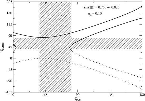
Figure 1: The “experimentally” determined (output) values for $\gamma$, as a function of its “true” value. The curves correspond to a $2\sigma$ deviation in both $\sin{2\beta}$ and $\sin{(2\beta+\gamma)}$. The allowed region between the dotted (filled) curves corresponds to $2\beta+\gamma$ in the first quadrant (second) quadrant. The hatched horizontal and vertical regions correspond to the currently allowed range, $37^{\circ}\leq\gamma\leq 80^{\circ}$. Here we assume that $\sin{2\beta}=0.750\pm 0.025$ and that the error on $\sin{(2\beta+\gamma)}$ is $0.1$.

Of course, the solution $\gamma_{\text{output}}=\gamma_{\text{true}}$ is included in the figure. Less obvious is the inclusion of the solution $\gamma_{\text{output}}=\pi-2\arcsin{{a_{\beta}}_{cv}}-\gamma_{\text{true}}$, which has to do with the discrete ambiguities to be discussed in subsection II.3. The point is that $\sin{\phi}=\sin{(\pi-\phi)}$ and, therefore, a measurement of $a_{\phi}$ is invariant under the transformation $\gamma\rightarrow\pi-4\beta-\gamma$.

Under the assumptions described, FIG. 1 tells us that, if $\gamma$ lies within its SM allowed range, a measurement of $\sin{(2\beta+\gamma)}$ will essentially not help us in constraining $\gamma$ any further. Of course, there is no good reason to take the central value of $a_{\beta}$ to determine the true value of $\beta$; nor is there any good reason to assume that the central value determined experimentally for $a_{\phi}$ will turn out to correspond to the true values for $\beta$ and $\gamma$. In fact, the measurement may hit the tail of the statistics. Also, the limiting curves in FIG. 1 correspond to rather conservative bounds, since they were found using the extreme values on both $a_{\beta}$ and $a_{\phi}$. This does not, however, affect the qualitative conclusions we will draw. Changing the central value ${a_{\beta}}_{cv}$ to $0.65$ (0.85) would alter FIG. 1 only slightly and would would not change our conclusion that, if the SM holds, essentially no new information will be gained.

This is one of our main points: with the errors of $\sigma_{a_{\beta}}=0.025$ and $\sigma_{a_{\phi}}=0.1$, we are unlikely to gain new information on $\gamma$. Nevertheless, as we will discuss in section III, such a measurement is useful in constraining new physics.

The situation improves dramatically as the experimental errors get smaller. We illustrate this point in FIG. 2, were we take ${a_{\beta}}_{cv}=0.75$ and we consider a factor of two improvement in the errors: $\sigma_{a_{\beta}}=0.0125$, $\sigma_{a_{\phi}}=0.05$, requiring an upgrade of the B factory.

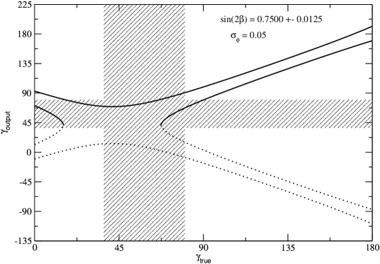
Figure 2: Same as FIG. 1, but with $\sin{2\beta}=0.7500\pm 0.0125$ and with an error on $\sin{(2\beta+\gamma)}$ of $0.05$.

Let us illustrate the various possibilities with a few examples. In Example 1 we assume that the measurements yield the 95% C.L. ranges of $0.7\leq a_{\beta}\leq 0.8$ and $0.6\leq a_{\phi}\leq 1.0$ (this corresponds to FIG. 1 with $\gamma_{\text{true}}\sim 78^{\circ}$). The possibility that $\phi$ is in the first quadrant leads to a lower limit $\gamma\geq-16^{\circ}$, while the second quadrant leads to an upper limit $\gamma\leq 99^{\circ}$. Moreover, the direct CP-violating parameter $\epsilon^{\prime}_{\text{B2}}$ is consistent with zero. If the experimental results turn out to be as in this example, we learn absolutely nothing within the SM. (However, as we will see in section III, the upper limit could constrain some extreme new physics.)

In Example 2 we assume that the prospective 95% C.L. experimental ranges are $0.725\leq a_{\beta}\leq 0.775$ and $0.7\leq a_{\phi}\leq 0.9$ (this corresponds to FIG. 2 with $\gamma_{\text{true}}\sim 78^{\circ}$). For $\phi$ in the first quadrant, Eq. (7) gives $-6^{\circ}\leq\gamma\leq 18^{\circ}$; for $\phi$ in the second quadrant, Eq. (6) gives $65^{\circ}\leq\gamma\leq 89^{\circ}$. When compared with the currently allowed range for $\gamma$ in Eq. (4), we are able to exclude the region $37^{\circ}\leq\gamma\leq 65^{\circ}$. Clearly this comes about because of the upper bound on $a_{\phi}$; as this upper bound comes away from $1.0$, we exclude more and more of the low values of $\gamma$. While we learn about $\gamma$, $\epsilon^{\prime}_{\text{B2}}$ remains consistent with zero.

The opposite could also occur. To illustrate this point, let us consider Example 3 where we assume the measurements to yield the 95% C.L. ranges $0.725\leq a_{\beta}\leq 0.775$ and $0.8\leq a_{\phi}\leq 1.0$ (this corresponds to FIG. 2 with $\gamma_{\text{true}}\sim 67^{\circ}$). In this case we obtain $2^{\circ}\leq\gamma$ for $\phi$ in the first quadrant, and $\gamma\leq 80^{\circ}$ for $\phi$ in the second quadrant. Here, while we gain no information on $\gamma$, we will have a signal of direct CP violation because $0.025\leq\epsilon^{\prime}_{\text{B2}}\leq 0.275$.

It is also possible that, in the presence of new physics, $\gamma_{\text{true}}$ is not consistent with the constraints from Eq. (4). As Example 4 let us consider $\gamma_{\text{true}}=105^{\circ}$ in FIG. 1. This corresponds to the prospective 95% C.L. ranges $0.7\leq a_{\beta}\leq 0.8$ and $0.25\leq a_{\phi}\leq 0.65$. These lead to $-39^{\circ}\leq\gamma\leq-4^{\circ}$, for $\phi$ in the first quadrant, and to $86^{\circ}\leq\gamma\leq 121^{\circ}$, for $\phi$ in the second quadrant. This would be an indication of physics beyond the SM, although, as discussed below in subsection II.3, the ambiguity induced by the strong phase might prevent a definitive conclusion. To phrase our conclusion differently: the measurement of $\sin{(2\beta+\gamma)}$ could, in principle, distinguish values of $\gamma$ consistent with the Standard Model from values of $\gamma$ requiring new physics.

II.3 The impact of strong phases

Thus far we have assumed that a clean measurement of $\sin{(2\beta+\gamma)}$ will be available. However, the presence of strong phases introduces discrete ambiguities which we will now discuss. The Dunietz Dun98 and KL KL methods involve final states which, although they are not CP eigenstates, can be accessed by both $B^{0}$ and $\overline{B^{0}}$. Moreover, as pointed out above, these decays involve only one weak phase because they are driven by the purely tree-level quark decay schemes $b\rightarrow ucs$ and $b\rightarrow ucd$, respectively. The importance of decays with these characteristics was first pointed out by Aleksan, Dunietz, Kayser, and Le Diberder ADKL , who showed that measuring the four decays $\{B^{0},\overline{B^{0}}\}\rightarrow\{f,\bar{f}\}$ enables the determination of

$$s_{\pm}\equiv\sin{(\phi\pm\Delta)},$$ (10)

where $\Delta$ is a strong phase, and $\phi$ is a weak phase (which coincides with $2\beta+\gamma$ in the Dunietz Dun98 and KL KL methods). Unfortunately, knowing $s_{\pm}$ does not in general determine the sign of $\cos{(\phi\pm\Delta)}$, meaning that

$$\sin^{2}{\phi}=\frac{1}{2}\left[1+s_{+}s_{-}\mp\sqrt{(1-s_{+}^{2})(1-s_{-}^{2})}\right],$$ (11)

can be confused with

$$\cos^{2}{\Delta}=\frac{1}{2}\left[1+s_{+}s_{-}\pm\sqrt{(1-s_{+}^{2})(1-s_{-}^{2})}\right].$$ (12)

Thus, we have in general an eightfold ambiguity due to the three symmetries BLS

$$\sin^{2}{\phi} \longleftrightarrow \cos^{2}{\Delta},$$ (13a)

$$\sin{\phi} \longleftrightarrow -\sin{\phi},$$ (13b)

$$\sin{\phi} \longleftrightarrow \sin{(\pi-\phi)}.$$ (13c)

Alternatively, we may view the eightfold ambiguity as resulting from the operations Soffer

$$\phi\rightarrow\Delta+\pi/2 \Delta\rightarrow\phi-\pi/2,$$ and (14a)

$$\phi\rightarrow\phi+\pi, \Delta\rightarrow\Delta+\pi,$$ and (14b)

$$\phi\rightarrow\pi-\phi, \Delta\rightarrow-\Delta.$$ and (14c)

The first of these ambiguities is the most serious if we cannot constrain the value of $\Delta$.

In fact, the value of $\Delta$ depends on the details of the final state scattering matrix and, thus, is difficult to predict. Beneke, Buchalla, Neubert, and Sachrajda BBNS , developing on the color transparency arguments of Bjorken BJ , have argued that the strong phases in $B_{d}\rightarrow D$ decays are small. On the other hand, a recent analysis by CLEO of the $B_{d}\rightarrow D\pi$ decays CLEO02 suggests the presence of final state interactions, with a strong phase $16.5^{\circ}<\delta_{I}<38.1^{\circ}$ at the $90\%$ C.L. This result can be understood as a large rescattering contribution and thus a sizeable strong phase for the color-suppressed decay to $D^{0}\pi^{0}$, which then shows up in the isospin analysis as a phase difference $\delta_{I}$ between the $I=1/2$ and the $I=3/2$ final states. As a result the final state $D^{+}\pi^{-}$ is expected to have a non-zero strong phase, probably smaller than $\delta_{I}$.

Dunietz’s proposal to determine $\sin(2\beta+\gamma)$ involves the relative strong phase between the $b\rightarrow c\bar{u}d$ and $\bar{b}\rightarrow\bar{u}c\bar{d}$ contributions to $B_{d}(\overline{B_{d}})\rightarrow D^{(*)+}\pi^{-}$. While these are not color-suppressed, there may still be significant rescattering from excited final states, such as $D^{(*)}\rho$. However, since the two decay amplitudes are related (essentially by the interchange of c and u) the same final states are involved for both of them and, so, the relative strong phase might be expected to be smaller than either one.

Let us now assume that the true value of $\Delta$ is very small but that we are not allowed to assume this fact in the analysis of the experiment. (Indeed, one does not wish for the extraction of $\sin{(2\beta+\gamma)}$ to be hampered by theoretical arguments, especially if it turns out to uncover a potential signal of new physics.) Then we have a confusion between $\sin^{2}{\phi}$ and $\cos^{2}{\Delta}\sim 1$. As an example, consider the possibility that $\phi=145^{\circ}$, corresponding to $\sin{\phi}=0.57$. The ambiguity mentioned implies that, even within the Standard Model, the experimental results do not allow us to determine whether $\phi=145^{\circ}$ and $\Delta=0$, or $\phi=90^{\circ}$ and $\Delta=\pm 55^{\circ}$. This is an important problem because, as illustrated above, an upper bound on $a_{\phi}=\sin{(2\beta+\gamma)}$ can be used to exclude low values of $\gamma$.

This ambiguity has no effect on the SM region of FIG. 1 since there $\sin^{2}{\phi}$ is consistent with $1$ anyway. The opposite occurs with FIG. 2, where it appears that, for large values of $\gamma_{\text{true}}$, the analysis ($\gamma_{{\text{output}}}$) can rule out small values of $\gamma$. This occurs because there is an upper limit on $\sin^{2}{\phi}$. Unfortunately, the presence of the ambiguity in Eq. (13a) eliminates this upper limit and the smaller values of $\gamma$ are allowed. This is illustrated in FIG. 3, where we have combined the allowed region of FIG. 2 with the region allowed by the ambiguity $\sin^{2}{\phi}\leftrightarrow\cos^{2}{\Delta}$, with $0.9\leq\cos{\Delta}\leq 1$.

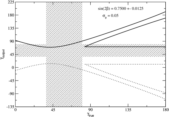
Figure 3: Same as FIG. 2, but including the ambiguity $\sin^{2}{\phi}\leftrightarrow\cos^{2}{\Delta}$, with $0.9\leq\cos{\Delta}\leq 1$.

As noted in Example 4, if we allow for the possibility of large new physics, then $\gamma$ may be outside the SM allowed values. This can also be seen from FIG. 2 where the whole SM range is ruled out if $\gamma_{\text{true}}>91^{\circ}$. However, the exchange in Eq. (13a) allows $a_{\phi}$ to be between $0.9$ and $1$ and, thus, most of the SM range is allowed, as seen in FIG. 3. Nevertheless, since the same interchange leads to a large value for $\Delta$, which we consider very unlikely, this could be considered as a strong indication of new physics.

We should also dispel two common misconceptions. It is often mentioned that one may remove the ambiguities due to $\Delta$ by comparing two different final states. For example, we could compare the results in $B_{d}\rightarrow D^{\pm}\rho^{\mp}$ with those in $B_{d}\rightarrow D^{\ast\pm}\rho^{\mp}$, thus identifying the strong phases. However, such a statement carries the hidden assumption that the distinction between the two strong phases is experimentally feasible. Given the expected experimental precision and assuming that the strong phases are indeed small, this may not work in practice.

One other common idea concerns the usefulness of a large final state phase in improving the sensitivity of a measurement of $\sin{(2\beta+\gamma)}$ to the phase $\gamma$. Recall that, as we have seen above, using the current SM ranges for $\beta$ and $\gamma$, a measurement of $\sin{(2\beta+\gamma)}$ is not very sensitive to the different values for $\gamma$. This is mainly due to the fact that $\sin{(2\beta+\gamma)}$ lies close to one for a good portion of the allowed range, where it is less sensitive to small differences in $\gamma$. One could think that, given that the measurements involve $\sin{(2\beta+\gamma\pm\Delta)}$, a large value for $\Delta$ would overcome this obstacle. This is not the case. The point is that, although the sensitivities of $s_{+}$ and $s_{-}$ to the phase $\gamma$ are indeed improved for large values of $\Delta$, these improvements cancel in the “inversion procedure” described in Eq. (11) that leads from these observables to the value of $\sin{(2\beta+\gamma)}$ which we wish to know.

We conclude that, in the SM, the final-state phases cannot improve the sensitivity of $a_{\phi}$ to the phase $\gamma$. Contrary to what one may think, if these phases are close to zero they are actually an enormous nuisance, since in that case, and whatever the value of $\phi$, one cannot distinguish the true value of $a_{\phi}$ from the possibility that $a_{\phi}\leftrightarrow\cos{\Delta}\sim 1$, thus precluding the exclusion of small values of $\gamma$. We have also shown that, if the final-state phases are large, the sensitivity of $a_{\phi}\sim 1$ to the phase $\gamma$ is not improved at all. Nevertheless, in that case, we may be lucky in disentangling the strong phases by comparing different channels.

III Constraining new physics with $\sin{(2\beta+\gamma)}$

Up to now, we have assumed the SM and concentrated our attention on the capabilities of a measurement of $\sin{(2\beta+\gamma)}$ to improve our information on the CKM phase $\gamma$. We now turn to the capabilities of this measurement to constrain new physics effects.

It is likely that the most precise determination of the CKM parameters in the next two or three years will come from the measurements of the CP-violating assymetry in $B_{d}\rightarrow\psi K$ decays and from the measurements of $\Delta m_{d}/\Delta m_{s}$. These determine the element $\tilde{V}_{td}$ with phase $\tilde{\beta}$ and magnitude

$$\left|\frac{\tilde{V}_{td}}{V_{ts}}\right|=\xi\sqrt{\frac{\Delta m_{d}}{\Delta m_{s}}\,\frac{m_{Bs}}{m_{Bd}}}.$$ (15)

The factor $\xi$ is 1 in the SU(3) limit and has been calculated on the lattice to be $1.15\pm 0.04$ UKQCD , but more theoretical work is needed to get the corrections to the quenched approximation Kron02 .

As an example, we consider the possibility that $\Delta m_{s}$ is found to be $20ps^{-1}$, $0.7\leq\sin 2\tilde{\beta}\leq 0.8$, and $1.08\leq\xi\leq 1.22$, with ranges corresponding to a 95% C.L. We assume that the major error in applying Eq. (15) is the theoretical error in $\xi$, since the experimental error in $\Delta m_{s}$ is expected to be very small, once it is measured BPTevatron . These two constraints define the region of $(\tilde{\rho},\tilde{\eta})$ shown by the solid line in FIG. 4.

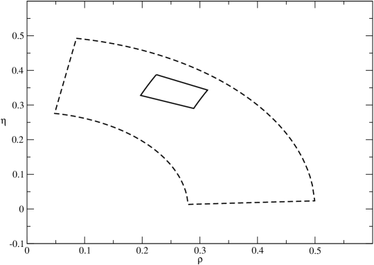
Figure 4: The solid curve shows the allowed region in the $(\rho,\eta)$ plane based on assumed mixing data with $\Delta m_{s}=20ps^{-1}$. The dashed lines show the constraints from assumed decay data.

The case where $\Delta m_{s}=30ps^{-1}$ would appear as a similar region displaced to the right and downward, but with similar structure.

We now look at the constraints that can be placed on $(\rho,\eta)$ solely on the basis of $B$ decays, in contrast to the $\tilde{V}_{td}$-based anaysis, that depended entirely on mixing. The magnitude of $V_{ub}$ is determined from semileptonic decays and its phase $\gamma$ is determined by comparing $\sin(2\tilde{\beta}+\gamma)$ with $\sin 2\tilde{\beta}$, as discussed in the previous sections. For our example, we assume that $0.28\leq\sqrt{\rho^{2}+\eta^{2}}\leq 0.5$ at the 95% C.L. This is an estimate of the present theoretical error Hock01 , and we believe that no great progress in reducing this error is likely to occur in the near future. To draw the constraints from decay we use $\sin(2\tilde{\beta})=0.75$, ${a_{\phi}}_{cv}=0.98$, $\sigma_{a_{\phi}}=0.1$, and allow $a_{\phi}$ to vary within the 95% C.L. range $0.78\leq a_{\phi}\leq 1$. This means that, by construction, the central value of $\gamma$ corresponds to the central value of $(\tilde{\rho},\tilde{\eta})$ in the example above, while $\tilde{\beta}$ is held fixed at $\arcsin{(0.75)}/2$. The resulting constraints on $(\rho,\eta)$ from decay are shown as dashed lines in FIG. 4 (the limits on $\gamma$ shown in FIG. 4 are slightly more restrictive than the corresponding ones shown in FIG. 1 because here we fix the value of $\tilde{\beta}$). We note that, in this case, the ambiguity from the strong phase disappears, assuming that it is not too different from zero.

As a result of new physics, the value from mixing may be different from the value from decay. As an example, we consider the possibility that the new physics only shows up as a contribution to the $B_{d}-\overline{B_{d}}$ mixing matrix $M_{12}$. We then write

$$M_{12}=M_{12}(\tilde{\rho},\tilde{\eta})=M_{12}(\rho,\eta)-Ye^{i\delta}M_{12},$$ (16)

where $Y$ measures the magnitude of the new physics as a fraction of $M_{12}$, and $\delta$ is the phase of the new physics relative to $2\tilde{\beta}$. Using the central values for $(\tilde{\rho},\tilde{\eta})$, each point $(\rho,\eta)$ along the boundary of the allowed region for decay, shown in FIG. 4, can be used to calculate values of $Y$ and $\delta$ Goto96 . The resulting limits on $Y$ as a function of $\delta$ are shown in FIG. 5.

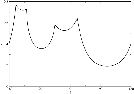
Figure 5: Limits on the new physics contributions to mixing. The limits corresponding to $-45^{\circ}<\delta<21^{\circ}$ ($-160^{\circ}<\delta<-129^{\circ}$) arises from the upper (lower) bound on $\gamma$.

We see that the constraint from $\sin(2\tilde{\beta}+\gamma)$ provides a constraint on $Y$ for values of $\delta$ in the ranges $(-160^{\circ},-129^{\circ})$ and $(-45^{\circ},21^{\circ})$. The cusps in Fig. 5 correspond to the corners of the dashed curve in Fig. 4 and, thus, to $2\sigma$ deviations in $\xi$ as well as in $a_{\phi}$. We have not considered constraints from kaon physics; for a portion of the region allowed for decays (that with smaller values of $\eta$), one would need to assume new physics in $K-\overline{K}$ mixing as well as in $B_{d}-\overline{B_{d}}$ mixing.

As mentioned before, barring the ambiguity due to the strong phase, smaller errors may allow us to detect new physics, even if $\gamma$ were not too far outside the range currently allowed in the SM. We illustrate this point by repeating the procedure described above, but with prospective measurements of $a_{\beta}=0.7500\pm 0.0125$ and $a_{\phi}=0.66\pm 0.05$ (this corresponds to $\gamma_{\text{true}}\sim 90^{\circ}$ in FIG. 2, leading to two separate regions for $\gamma_{1}$ and $\gamma_{2}$). In this case, we can see from FIG. 6 that the mixing infered $(\tilde{\rho},\tilde{\eta})$ region (bounded by the solid lines) is completely disjoint from the decay infered $(\rho,\eta)$ regions (bounded by the dashed lines).

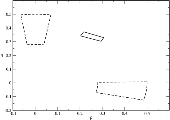
Figure 6: The solid curve shows the allowed region in the $(\rho,\eta)$ plane based on assumed mixing data with $\Delta m_{s}=20ps^{-1}$. The dashed lines show the constraints from assumed decay data.

As a result, $Y$ is different from zero for some value of $\delta$ in the ranges $(-160^{\circ},-130^{\circ})$ and $(-44^{\circ},18^{\circ})$, as shown in FIG. 7,

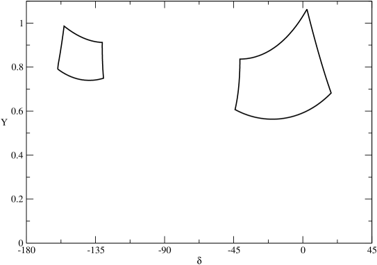
Figure 7: Possible values of the new physics contributions to mixing. The bounds corresponding to $-160^{\circ}<\delta<-130^{\circ}$ ($-44^{\circ}<\delta<18^{\circ}$) arise from $\phi$ in first (second) quadrant.

and we would have identified new physics. However, we must consider the ambiguity due to $\sin^{2}{\phi}\leftrightarrow\cos^{2}{\Delta}$. In this particular case, that leaves us with the option of believing in a rather large value for $Y$ or, alternatively, admitting that there is no new physics but the strong phase is large, between $45^{\circ}$ and $52^{\circ}$. We may hope that, as we learn more about the systematics of these decays, the arguments against such a large strong phase may become decisive.

IV Conclusions

In this paper we have considered what can be learned from prospective experiments on $\sin{(2\beta+\gamma)}$. We have not tried to simulate the future error analysis but, rather, by considering a few examples, have reached qualitative conclusions. Assuming the standard model is correct, one can find significant constraints on the value of $\gamma$ only if the error is $\sigma_{a_{\phi}}=0.05$ or less and, even then, stronger constraints are likely from the $\sin{2\beta}$ and $\Delta m_{s}$ experiments. On the other hand, if we allow for the possibility that there may be new physics contributions to $B_{d}-\overline{B_{d}}$ mixing, then comparing the results from experiments probing $\sin{(2\tilde{\beta}+\gamma)}$ with the results obtained from mixing (namely, $\sin{2\tilde{\beta}}$ and $\Delta m_{d}/\Delta m_{s}$) can provide significant constraints on the new physics contribution, and may even give an indication of the presence of such contributions.

- (1) N. Cabibbo, Phys. Rev. Lett. 10, 531 (1963); M. Kobayashi and T. Maskawa, Prog. Theor. Phys. 49, 652 (1973).
- (2) BABAR Collaboration, B. Aubert et. al., hep-ex/0207042.
- (3) Belle Collaboration, K. Abe et. al., hep-ex/0207098.
- (4) M. Gronau and D. London, Phys. Lett. B 253, 483 (1991).
- (5) G. C. Branco, L. Lavoura, and J. P. Silva, CP Violation (Oxford University Press, Oxford, 1999).
- (6) The impact of mixing in decay was first pointed out in C. C. Meca and J. P. Silva, Phys. Rev. Lett. 81, 1377 (1998). Extensive studies appear in A. Amorim, M. G. Santos, and J. P. Silva, Phys. Rev. D 59, 056001 (1999); J. P. Silva and A. Soffer, Phys. Rev. D 61, 112001 (2000).
- (7) B. Kayser and D. London, Phys. Rev. D 61, 116013 (2000).
- (8) See also D. Atwood and A. Soni, e-Print Archive: hep-ph/0206045.
- (9) I. Dunietz, Phys. Lett. B 427, 179 (1998).
- (10) D. London, N. Sinha, and R. Sinha, Phys. Rev. Lett. 85, 1807 (2000).
- (11) See, however, A. S. Kronfeld and S. M. Ryan, hep-ph/0206058, who call into question the value commonly used for the SU(3) breaking parameter.
- (12) A. Ali and D. London, DESY preprint number DESY-00-026, hep-ph/0002167, published in the proceedings of 3rd Workshop on Physics and Detectors for DAPHNE (DAPHNE 99), Italy (1999).
- (13) A. Höcker, H. Lacker, S. Laplace and F. Le Diberder, Eur. Phys. J. C 21, 225 (2001); ibid. hep-ph/0112295.
- (14) L. Wolfenstein and F. Wu, Europhys. Lett. 58, 49 (2002).
- (15) For a detailed explanation of this type of ‘direct CP violation without strong phases’ see pages 55, 80 and (for the relation with ) 102 of reference BLS .
- (16) C. Voena and W. A. Walkowiak, private communication. The results of these studies predict an error for which is roughly twice the error estimated in The BaBar physics book, edited by P. F. Harrison and H. R. Quinn (SLAC, Stanford, 1998).
- (17) R. Aleksan, I. Dunietz, B. Kayser, and F. Le Diberder, Nuc. Phys. B 361, 141 (1991).
- (18) See A. Soffer, Phys. Rev. D 60, 054032 (1999), for the corresponding ambiguities in the methods of the following references: M. Gronau and D. Wyler, Phys. Lett. B 265, 172 (1991); D. Atwood, I. Dunietz, and A. Soni, Phys. Rev. Lett. 78, 3257 (1997). See also reference BLS .
- (19) M. Beneke, G. Buchalla, M. Neubert, and C. T. Sachrajda, Phys. Rev. Lett. 83, 1914 (1999); ibid Nucl. Phys. B 591, 313 (2000).
- (20) J. D. Bjorken, Nucl. Phys. Proc. Suppl. 11, 325 (1989).
- (21) CLEO Collaboration, S. Ahmed et al., hep-ex/0206030.
- (22) L. Lellouch and C. J. Lin , UKQCD Collaboration, Phys. Rev. D 64, 094501 (2001). See also ref. Kron02 .
- (23) K. Anikeev et al., “ Physics at the Tevatron: Run II and Beyond,” hep-ph/0201071, FERMILAB-Pub-01/197, http://www-theory.lbl.gov/Brun2/report/.
- (24) This general approach was shown graphically in T. Goto, T. Nihei and Y. Okada, Phys. Rev. D 53, 5233 (1996); ibid., Phys. Rev. D 54, 5904 (1996).