Exclusive Nonleptonic $B$ Decays from QCD Light-Cone Sum Rules

Abstract

We are going to review recent advances in the theory of exclusive nonleptonic B decays. The emphasis is going to be on the factorization hypothesis and the role of nonfactorizable contributions for nonleptonic B decays. In particular, we will discuss more in detail calculations of nonfactorizable contributions in the QCD light-cone sum rule approach and their implications to the $B\rightarrow\pi\pi$ and $B\rightarrow J/\psi K$ decays.

1 Exclusive Nonleptonic $B$ Decays and Factorization

Exclusive nonleptonic decays represent a great challenge to theory. They are complicated by the hadronization of final states and strong-interaction effects between them. Today measurements have already reached sufficient precision to examine our knowledge of these effects. In order to make real use of data in the determination of fundamental parameters and in testing of the Standard Model, we are forced to provide a more accurate estimation of nonperturbative quantities, such as the matrix elements of weak operators.

At the first sight, the nonleptonic $B$ meson decay seems to be simple, as far as we essentially consider this decay as a weak decay of heavy $b$ quark. We are encouraged to use this argument by the facts that the $b$ quark mass is heavy compared to the intrinsic scale of strong interactions and that the $b$ quark decays fast enough to produce energetic constituents, which separate without interfering with each other. This naive picture was supported by the color-transparency argument Bjorken and natural application to nonleptonic two-body decays emerged under the name the naive factorization (discussed in detail below). However, although predictions from the naive factorization are in relatively good agreement with the data (apart from the color-suppressed decays), the naive factorization provides no insight into the dynamical background of exclusive nonleptonic decays.

The theoretical discussion of the nonleptonic decay starts with the effective weak Hamiltonian, which summarizes our knowledge of weak decays at low scales (for a review see BBL ):

$${\cal H}_{weak}=\frac{G_{F}}{\sqrt{2}}\,V_{Qq_{1}}V_{q_{2}q_{3}}\left[C_{1}(\mu){\cal O}_{1}+C_{2}(\mu){\cal O}_{2}+.....\right]\,.$$ (1)

The $V$s represent the Cabibbo-Kobayashi-Maskawa (CKM) matrix elements specified for the particular heavy-quark decay $Q\rightarrow q_{1}q_{2}\overline{q}_{3}$. Strong-interaction effects above some scale $\mu\sim m_{b}$ are retained in the Wilson coefficients $C_{i}(\mu)$. These coefficients are perturbatively calculable and therefore well known. Actually, the weak theory without strong corrections and QED effects knows only the operator ${\cal O}_{1}$, and in that case $C_{1}(M_{W})=1$ and $C_{2}(M_{W})=0$. The operator ${\cal O}_{2}$, defined in (2), emerges after taking the gluon exchange into account and therefore its contribution is suppressed as $C_{2}(\mu)\sim\ln(M_{W})/\ln(\mu)$.

The main problem persists in the calculation of matrix elements of operators ${\cal O}_{i}$ in a particular process. In (1) we retain only the leading operators ${\cal O}_{1}$ and ${\cal O}_{2}$ and suppress explicitly so called penguin operators, ${\cal O}_{i=3,...,10}$. Being multiplied by, in principle, small Wilson coefficients, the penguin operators usually can be neglected (except for the penguin-dominated decays), but could be extremely important for detection of $CP$ violation in $B$ decay Neubert ; Fleischer ; Mannel .

The four-quark operators ${\cal O}_{1}$ and ${\cal O}_{2}$ differ only in their color structure:

$${\cal O}_{1}=(\overline{q}_{1{i}}\Gamma_{\mu}Q_{{i}})(\overline{q}_{2{j}}\Gamma^{\mu}q_{3{j}})\,,\qquad\qquad{\cal O}_{2}=(\overline{q}_{1{i}}\Gamma_{\mu}Q_{{j}})(\overline{q}_{2{j}}\Gamma^{\mu}q_{3{i}})\,,$$ (2)

where $i$ and $j$ are color indices, and $\Gamma_{\mu}=\gamma_{\mu}(1-\gamma_{5})$. The color-mismatched operator ${\cal O}_{2}$ can be projected to the color singlet state by using the relation $\delta_{ij}\delta_{kl}=1/N_{c}\,\delta_{il}\delta_{jk}+2\,(\lambda^{a}/2)_{il}\,(\lambda^{a}/2)_{jk}$, as

$${\cal O}_{2}=\frac{1}{N_{c}}{\cal O}_{1}+2\,\tilde{{\cal O}}_{1}\,.$$ (3)

This projection, as can be seen from (3), results in a relative suppression of the ${\cal O}_{2}$ operator contribution of the order $1/N_{c}$ ($N_{c}$ is the number of colors) and in the appearance of the new operator $\tilde{{\cal O}}_{1}$ with the explicit color SU(3) matrices $\lambda^{a}$:

$$\tilde{{\cal O}}_{1}=(\overline{q}_{1i}\Gamma_{\mu}\frac{\lambda^{a}}{2}Q_{i})(\overline{q}_{2j}\Gamma^{\mu}\frac{\lambda^{a}}{2}q_{3j})\,.$$ (4)

Depending on the process involved, the operators ${\cal O}_{1}$ and ${\cal O}_{2}$ can exchange their roles, and then it is customary to define the effective parameters $a_{1}$ and $a_{2}$ as

$$a_{1}=C_{1}(\mu)+\frac{1}{N_{c}}C_{2}(\mu)\,,\qquad\qquad\qquad a_{2}=C_{2}(\mu)+\frac{1}{N_{c}}C_{1}(\mu)\,.$$ (5)

These parameters distinguish between three classes of decay topologies:
- class-1 decay amplitude, where a charged meson is directly produced in the weak vertex; i.e. in the quark transition $b\rightarrow ud\overline{u}$ with ${\cal O}_{1}=(\overline{d}\Gamma_{\mu}u)(\overline{u}\Gamma^{\mu}b)$:

$${\cal A}(B\rightarrow\pi^{+}\pi^{-})\sim a_{1}\langle O_{1}\rangle\,,$$ (6)

- class-2 decay amplitude, where a neutral meson is directly produced, i.e. in the quark transition $b\rightarrow cs\overline{c}$ with ${\cal O}_{2}=(\overline{c}\Gamma_{\mu}c)(\overline{s}\Gamma^{\mu}b)$:

$${\cal A}(B^{+}\rightarrow J/\psi K^{+})\sim a_{2}\langle O_{2}\rangle\,,$$ (7)

- class-3 decay amplitude, where both cases are possible, but this amplitude is however connected by isospin symmetry with the class-1 and class-2 decays; i.e. in the quark transition $b\rightarrow cs\overline{u}$ with ${\cal O}_{1}=(\overline{c}\Gamma_{\mu}u)(\overline{s}\Gamma^{\mu}b)$:

$${\cal A}(B^{-}\rightarrow D^{0}K^{-})\sim(a_{1}+xa_{2})\langle O_{1}\rangle\,,$$ (8)

where $x$ denotes the nonperturbative factor being equal to one in the flavor-symmetry limit.

The effective parameters $a_{1}$ and $a_{2}$ are defined with respect to the naive factorization hypothesis, which assumes that the nonleptonic amplitude can be expressed as the product of matrix elements of two hadronic (bilinear) currents, for example:

$$\langle\pi^{+}\pi^{-}|(\overline{d}\Gamma_{\mu}u)(\overline{u}\Gamma^{\mu}b)|B\rangle\rightarrow\langle\pi^{-}|(\overline{d}\Gamma_{\mu}u)|0\rangle\langle\pi^{+}|(\overline{u}\Gamma^{\mu}b)|B\rangle$$ (9)

and that there is no nonfactorizable exchange of gluons between the $\pi^{-}$ and the $|\pi^{+}B\rangle$ system. Effectively, that means that the ’nonfactorizable’ matrix element of the $\tilde{{\cal O}}_{1}$ operator (4), is vanishing, due to the projection of the colored current to the physical colorless state.

1.1 Nonfactorizable Contributions

The effective parameters $a_{1}$ and $a_{2}$ could be generalized to parametrize also the nonfactorizable strong-interaction effects, for example gluon exchanges between bilinear currents (i.e. in (9)) which introduce nonvanishing contribution from ${\tilde{\cal O}}$ operators. Schematically, in the large $N_{c}$ limit,

$$a_{1} = C_{1}(\mu)+\frac{1}{N_{c}}C_{2}(\mu)+2C_{2}(\mu)\xi^{nf}_{2}(\mu)\,,$$ (10)

$$a_{2} = C_{2}(\mu)+\frac{1}{N_{c}}C_{1}(\mu)+2C_{1}(\mu)\xi^{nf}_{1}(\mu)\,,$$ (11)

where we have explicitly indicated that the nonfactorizable contribution to the class-1 and class-2 decays $\xi^{nf}_{i=1,2}$, do not necessarily need to be the same, and also they can be process dependent quantities, which will be discussed later. Theoretically, nonfactorizable effects are desirable in order to cancel explicit the $\mu$ dependence of $C_{i}(\mu)$ and therefore of the $a_{i}$’s. All physical quantities are $\mu$ independent, and because there is no explicit $\mu$ dependence of the matrix elements $\langle{\cal O}_{i}\rangle$ multiplying $C_{i}(\mu)$, there must be some underlying mechanism to cancel the explicit $\mu$ dependence of $a_{i}$’s persisting in the factorization approach. In the calculation of the Wilson coefficients beyond the leading order, also the renormalization scheme dependence is presented Buras . Naturally, the parameter $a_{2}$ is more sensitive on the value of the factorization scale and on the renormalization scheme, due to the similar magnitude and different sign of the $C_{2}(\mu)$ and $1/N_{c}C_{1}(\mu)$ terms (calculated in the NDR scheme and for $\Lambda_{\overline{MS}}^{(5)}=225\,GeV$, the Wilson coefficients have the following values: $C_{1}(m_{b})=1.082$ and $C_{2}(m_{b})=-0.185$ BBL ). This means also that $a_{2}$ is more sensitive to any additional nonperturbative long-distance contributions.

The global fit of $a_{1}$ and $a_{2}$ parameters to the $B$ meson experimental data performed in NS , has shown that the $a_{1}$ coefficient, being essentially proportional to $C_{1}(\mu)\sim 1$, is in the expected theoretical range:

$$a_{1}\sim 1.05\pm 0.10\,,$$ (12)

while $a_{2}$ has the fitted value of

$$a_{2}\sim 0.25\pm 0.05\,.$$ (13)

Compared with the theoretical values calculated with the $C_{1}$ and $C_{2}$ stated above, we note that both fitted values show no explicit indication that there is a significant nonfactorizable contribution in $B$ decays. This confirms the naive factorization picture, although the simple extrapolation of results in $D$ decays to the $B$ case would suggest that the $a_{2}$ coefficient could be negative, meaning a nontrivial cancellation of the $1/N_{c}$ terms and dominance of (negative) $C_{2}(\mu)$ in (11). The negative value of $a_{2}$ in $D$ decays has found its confirmation in the large $N_{c}$ hypothesis of neglecting the higher order $1/N_{c}$ terms, BGR , and in the QCD sum rule calculation BS , where the cancellation of the $1/N_{c}$ part with the explicitly calculated nonfactorizable terms was verified.

However, there are additional indications that nonfactorizable contributions in $B$ decays cannot be simply neglected and deserve to be investigated. New experimental data on $B$ mesons indicate nonuniversality of the $a_{2}$ parameter and the strong final-state interaction phases in the color-suppressed class-2 decays being proportional to $a_{2}$ NP .

Therefore, the nonfactorizable contributions must play an important role in nonleptonic decays, particularly in the color-suppressed class-2 decays, such as the $B\rightarrow J/\psi K$ decay discussed in Sect.4.

1.2 Models for the Calculation of Nonfactorizable Contributions

Nowadays, there exist several approaches for the treatment of nonleptonic decays, which try to investigate the dynamical background and nonfactorizable contributions of such processes. The most exploited ones are the QCD-improved factorization, BBNS , and the PQCD approach KLS .

The PQCD approach claims the perturbativity of the two-body nonfactorizable amplitude if the Sudakov suppression is implemented into the calculation. The Sudakov form factor suppresses the configuration in which the soft gluon exchange could take place, and the amplitude is dominated by exchange of hard gluons and therefore perturbatively calculable.

A somewhat different method is applied in the QCD-improved factorization. This method provides the factorization formula that separates soft and hard contribution on the basis of large $m_{b}$ expansion. The leading nonfactorizable strong interaction can be then studied systematically, while soft (incalculable) contributions are suppressed by $\Lambda_{QCD}/m_{b}$. The method applies to class-1 decays and to class-2 decays under the assumption $m_{c}\ll m_{b}$.

None of these models take nonfactorizable soft $O(\Lambda_{QCD}/m_{b})$ corrections into account. These corrections can be brought under control by using the light-cone QCD sum rule method Khodja . This method is going to be discussed more in detail in what follows.

2 Light-Cone Sum Rules

All QCD sum rules are based on the general idea of calculating a relevant quark-current correlation function and relating it to the hadronic parameters of interest via a dispersion relation. Sum rules in hadron physics were already known before QCD was established (for a comprehensive introduction to sum rules see i.e. deRafael ), but have reached wide application in a calculation of various hadronic quantities in the form of so-called SVZ sum rules SVZ . The other type of sum rules, the light-cone QCD sum rules were established for calculation of exclusive amplitudes and form factors (CK and references therein).

2.1 Light-Cone Sum Rules vs SVZ Sum Rules

In order to illustrate application of the QCD sum rules and the main differences between SVZ sum rules and light-cone sum rules, we introduce an example.

One of the typical calculation using the SVZ sum rules is the estimation of the $B$ meson decay constant $f_{B}$. The starting point is a correlation function defined as

$$F(q^{2})=i\int d^{4}xe^{iqx}{\langle 0|}T\{m_{b}\overline{u}i\gamma_{5}b(x),m_{b}\overline{b}i\gamma_{5}u(0)\}{|0\rangle}\,.$$ (14)

In the Euclidean region of $q$ momenta, $q^{2}<0$, we can perform a perturbative calculation in terms of quarks and gluons by applying the short-distance operator-product expansion (OPE) to the correlation function $F(q^{2})$. The correlation function is then expressed via a dispersion relation in terms of the spectral function $\rho^{OPE}$, representing the perturbative part, and the quark and gluon condensates, i.e. $\langle q\overline{q}\rangle$, $\langle GG\rangle$, etc (see for example Reinders ):

$$F^{OPE}(q^{2})=\frac{1}{\pi}\int_{0}^{\infty}ds\frac{ImF^{OPE}(s)\,ds}{s-q^{2}}+A_{i}(s)\langle O|\Omega_{i}|0\rangle\,,$$ (15)

where

$$\frac{1}{\pi}ImF^{OPE}(s)=\rho^{OPE}(s)$$ (16)

and $A_{i}$ are perturbative coefficients in front of the vacuum condensates of operators $\Omega_{i}=\overline{q}q\,,GG\,,\overline{q}\lambda^{a}/2\sigma\cdot Gq$   , etc.

On the other hand, in the physical (Minkowskian) region, $q^{2}>0$, we insert the complete sum over hadronic states starting from the ground state $B$ meson, and use a defining relation for $f_{B}$ : $\langle m_{b}\overline{q}i\gamma_{5}b|B\rangle=f_{B}m_{B}^{2}$. The correlation function $F(q^{2})$ can then be written as

$$F^{hadron}(q^{2})=\frac{m_{B}^{4}f_{B}^{2}}{m_{b}^{2}-q^{2}}+\int_{s_{0}^{h}}^{\infty}\frac{\rho^{hadron}(s)\,ds}{s-q^{2}}\,,$$ (17)

where the hadronic spectral density $\rho^{hadron}$ contains all higher resonances and non-resonant states with the $B$ meson quantum numbers.

By applying the quark-hadron duality to these higher hadronic (continuum) states, which means assuming that we can replace the continuum of hadronic states, described by the hadronic spectral function $\rho^{hadron}(s)$ via a dispersion relation, by the spectral function calculated perturbatively in the $q^{2}<0$ region $\rho^{OPE}(s)$, we match both sides, $F^{OPE}(q^{2})=F^{hadron}(q^{2})$, and extract the needed quantity $f_{B}$. The replacement is done for $s>s_{0}^{B}$, where $s_{0}^{B}$ is an effective parameter of the order of the mass of the first excited $B$ meson resonance squared.

In a practical calculation one performs a finite power expansion in $\rho^{OPE}(s)$. To improve the convergence of the expansion, the Borel transform of both sides, $F^{OPE}(q^{2})$ and $F^{hadron}(q^{2})$, is considered, defined by the following limiting procedure

$${{\cal B}=lim\frac{1}{(n-1)!}(-q^{2})^{n}(\frac{d}{dq^{2}})^{n}}\quad\quad|q^{2}|,n\rightarrow\infty\,,{\frac{|q^{2}|}{n}}={M^{2}}\;\;fixed\,.$$ (18)

$M^{2}$ is so called Borel parameter. It is determined by the search for stability criteria in a sense that, on the one hand, excited and continuum states are suppressed (asks for smaller $M^{2}$) and, on the other hand, the reliable perturbative calculation is enabled (asks for larger $M^{2}$).

The general procedure of QCD sum rules is depicted on Fig. 1.

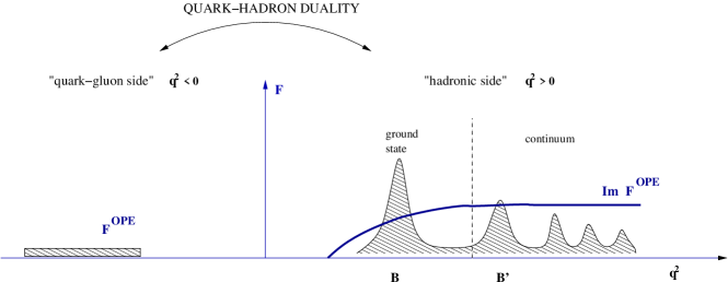
Figure 1: An illustration of the matching procedure in QCD sum rules

For calculating quantities which involve hadron interactions, such as for example the $B\rightarrow\pi$ form factor, the light-cone sum rules are more suitable Braun . The correlation function is now defined as a vacuum-to-pion matrix element:

$$F_{\mu}=i\int d^{4}xe^{-ipx}{\langle\pi(q)|}T\{\overline{u}\gamma_{\mu}b(x),m_{b}\overline{b}i\gamma_{5}d(0)\}{|0\rangle}\,.$$ (19)

The calculation follows by performing a light-cone OPE, an expansion in terms of the light-cone wave functions of increasing twist (twist = dimension - spin). Physically, it means that one performs an expansion in the transverse quark distances in the infinite momentum frame, rather than a short-distance expansion Braun . Instead of dealing with the vacuum-to-vacuum quark and gluon condensates (numbers) like in the SVZ sum rules, we have now to know the pion distribution amplitude (wave function). The leading twist-2 pion distribution amplitude, $\phi_{\pi}$ is defined as

$$\langle\pi(q)|\overline{u}(x)\gamma_{\mu}\gamma_{5}d(0)|0\rangle=-iq_{\mu}f_{\pi}\int_{0}^{1}due^{iuqx}\phi_{\pi}(u)\,.$$ (20)

Distribution amplitudes (DAs) describe distributions of the pion momentum over the pion constituents and $u$ denotes the fraction of this momentum, $0<u<1$ (for a comprehensive paper on the exclusive decays and the light-cone DAs see Brodsky ). The DAs represent a nonperturbative, noncalculable input and their form has to be determined by nonperturbative methods and/or somehow extracted from the experiment.

In the physical region of $(p-q)^{2}>0$ nothing changes in comparison to the SVZ sum rules. We insert the complete set of hadronic states with $B$ meson quantum numbers as before, and extract the $B\rightarrow\pi$ form factor from the relation: $\langle\pi(q)|\overline{u}\gamma_{\mu}b|B(p+q)\rangle=2f_{B\pi}^{+}(p^{2})q_{\mu}+...$. The matching procedure follows as described above.

3 Nonfactorizable Effects in the Light-Cone Sum Rules

Although the idea to apply QCD sum rules for calculating nonfactorizable contributions in nonleptonic $B$ decays is not the new one, earlier applications were facing some problems which have caused unavoidable theoretical uncertainties in their results Khodja . In the work Khodja , a new approach was introduced and we are going first to review its main ideas in the application to the $B\rightarrow\pi\pi$ decay.

3.1 Definitions

The correlator for the $B\rightarrow\pi\pi$ decay given in terms of two interpolating currents for the pion and the $B$ meson, $J_{\nu 5}^{(\pi)}=\overline{u}\gamma_{\nu}\gamma_{5}d$ and $J_{5}^{(B)}=m_{b}\overline{b}i\gamma_{5}d$ respectively, and relevant operators ${\cal O}_{1}=(\overline{d}\Gamma_{\mu}u)(\overline{u}\Gamma^{\mu}b)$ and $\tilde{{\cal O}}_{1}=(\overline{d}\Gamma_{\mu}\lambda^{a}/2u)(\overline{u}\Gamma^{\mu}\lambda^{a}/2b)$ looks like:

$$F_{\nu}(p,q,k)=\int d^{4}xe^{-i(p-q)x}\int d^{4}ye^{i(p-k)y}\langle 0|T\{J_{\nu 5}^{(\pi)}(y){\cal O}_{i}(0)J_{5}^{(B)}(x)\}|\pi(q)\rangle\,.$$ (21)

The transition is defined again between a vacuum and an external pion state. The situation is illustrated in Fig. 2.

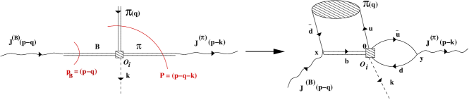
Figure 2: Sum rule calculation of the $B\rightarrow\pi\pi$ decay. The shaded oval region denotes nonperturbative input, $\pi$ meson distribution amplitude. The other pion and the $B$ meson are represented by the currents $J^{(\pi)}(p-k)$ and $J^{(B)}(p-q)$ respectively. The square represents the four-quark operators ${\cal O}_{i}$.

One can note an unphysical momentum $k$ coming out from the weak vertex. It was introduced in order to avoid the $B$ meson four-momenta before ($p_{B}=(p-q)$), and after ($P$) the decay to be the same, Fig. 2. In such a way, it was prevented that the continuum of light states enters the dispersion relation of the $B$ channel. States, like $D\overline{D}_{s}^{\ast}$ and $D^{\ast}\overline{D}_{s}$, have masses smaller than the ground state $B$ meson mass and spoil the extraction of the physical $B$ meson. These ’parasitic’ contributions have caused problems in the earlier application of the sum rules Khodja . There are several other momenta involved into the decay and we take $p^{2}=k^{2}=q^{2}=0$ and consider region of large spacelike momenta

$$|(p-k)^{2}|\sim|(p-q)^{2}|\sim|P^{2}|\gg\Lambda_{QCD}^{2}\,,$$ (22)

where the correlation function is explicitly calculable.

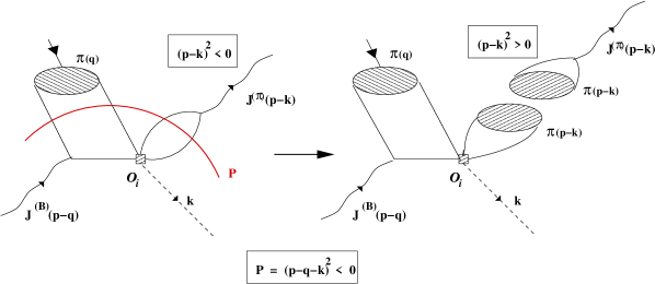
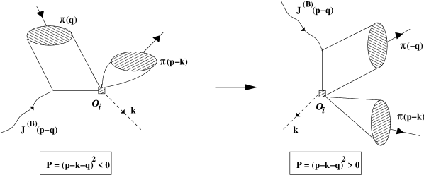
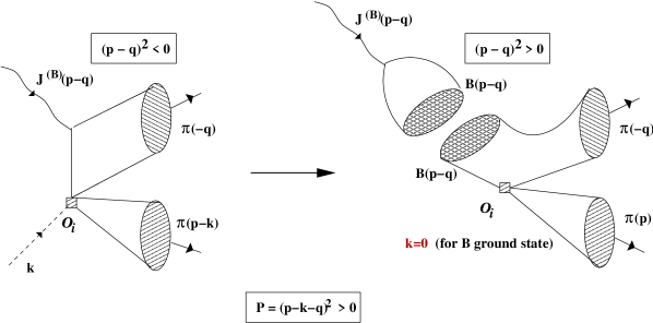
(a) Dispersion relation in the pion channel of momentum $(p-k)^{2}<0$ (b) Analytical continuation of $P^{2}$ to $P^{2}=m_{B}^{2}$ (c) Dispersion relation in the $B$ meson channel of momentum $(p-q)^{2}<0$

Figure 3: The light-cone sum rule procedure for exclusive decays

3.2 Procedure

The procedure which one performs is exhibited in Fig. 3. First, Fig. 3a, one makes a dispersion relation in a pion channel of momentum $(p-k)^{2}$ and applies the quark-hadron duality for this channel, as it was explained in Sect.2. Thereafter, to be able later to extract physical $B$ meson state, one has to perform an analytical continuation of $P$ momentum to its positive value, $P^{2}=m_{B}^{2}$. This procedure is analogous to the one in the transition from the spacelike to the timelike pion form factor, Fig. 3b. Finally, Fig. 3c, a dispersion relation in the $B$ channel of momentum $(p-q)^{2}$ has to be done, together with the application of the quark-hadron duality, now in the $B$ channel Khodja . In such a way we arrive to the double dispersion relation. Apart from somewhat more complicated matching procedure, the calculation otherwise follows in a standard way.

3.3 Results and Implications in the $B\rightarrow\pi\pi$ decay

In Khodja , first, the factorization of the ${\cal O}_{1}$ operator contribution in the $B\rightarrow\pi\pi$ decay was confirmed. The soft nonfactorizable contributions due to the $\tilde{\cal O}_{1}$ operator, which express the exchange of soft gluons between two pions in Fig. 2 were then calculated. Nonfactorizable soft contributions appear from the absorption of a soft gluon emerging from the light-quark loop $\overline{u}d$ in Fig. 2, by the distribution amplitude of the outcoming pion $\pi^{+}(-q)$ and there are of the higher, twist-3 and twist-4 order in comparison to the factorizable contributions.

Nonfactorizable soft corrections appeared to be numerically small ($\sim 1\%$) and suppressed by $1/m_{b}$. Therefore, their impact on the complete decay amplitude was shown to be of the same order as that of hard nonfactorizable contributions calculated in the QCD-improved factorization approach BBNS . Also, the calculation has shown no imaginary phase from the soft contributions, whereas aforementioned hard nonfactorizable contributions get small complex phase because of the final state rescattering due to the hard gluon exchange.

4 Nonfactorizable Effects for $B\rightarrow J/\psi K$

The $B\rightarrow J/\psi K$ decay was considered in mi . As it was emphasized at the beginning, this decay belongs to the color-suppressed class-2 decays in which one expects large nonfactorizable contributions. The confirmation of this assumption seems to be also found experimentally. Namely, there is a discrepancy between the experiment and the naive factorization prediction by at least a factor of 3 in the branching ratio. The Hamiltonian which describes the decay is given as

$$H_{W}=\frac{G_{F}}{\sqrt{2}}V_{cb}V_{cs}^{*}\left[(C_{2}(\mu)+\frac{1}{N_{c}}C_{1}(\mu)){\cal O}_{2}+2\,C_{1}(\mu)\tilde{{\cal O}}_{2}\right]\,,$$ (23)

with the operators ${\cal O}_{2}=(\overline{c}\Gamma_{\mu}c)(\overline{s}\Gamma^{\mu}b)$ and $\tilde{{\cal O}}_{2}=(\overline{c}\Gamma_{\mu}\frac{\lambda_{a}}{2}c)(\overline{s}\Gamma^{\mu}\frac{\lambda_{a}}{2}b)$. In the factorization approach, the matrix element of $\tilde{{\cal O}}_{2}$ vanishes, and the factorized matrix element of the operator ${\cal O}_{2}$ is given by

$$\langle J/\psi(p)K(q)|{\cal O}_{2}|B(p+q)\rangle = \langle J/\psi(p)|\overline{c}\Gamma_{\mu}c|0\rangle\langle K(q)|\overline{s}\Gamma^{\mu}b|B(p+q)\rangle$$ (24)

$$= 2\epsilon\cdot q\,m_{J/\psi}f_{J/\psi}F^{+}_{BK}(m_{J/\psi}^{2})\,.$$ (25)

$F^{+}_{BK}(m_{J/\psi}^{2})$ is the $B\rightarrow K$ transition form factor calculated using the light-cone sum rules, in a way enlightened in Sect.2.1 on the example of $B\rightarrow\pi$ form factor calculation, and $f_{J/\psi}$ is the $J/\psi$ decay constant. By evaluating numerically the $B\rightarrow J/\psi K$ branching ratio with the NLO Wilson coefficients used in Sec.1.1 and with the numerical input taken from mi , we arrive to

$${\cal B}(B\rightarrow J/\psi K)^{fact}=3.3\cdot 10^{-4}\,.$$ (26)

This has to be compared with the recent measurements exp

$${\cal B}(B^{+}\rightarrow J/\psi K^{+}) = (10.1\pm 0.3\pm 0.5)\cdot 10^{-4}\,,$$ (27)

$${\cal B}(B^{0}\rightarrow J/\psi K^{0}) = (8.3\pm 0.4\pm 0.5)\cdot 10^{-4}\,.$$ (28)

It is clear that there a discrepancy between the naive factorization prediction and the experiment.

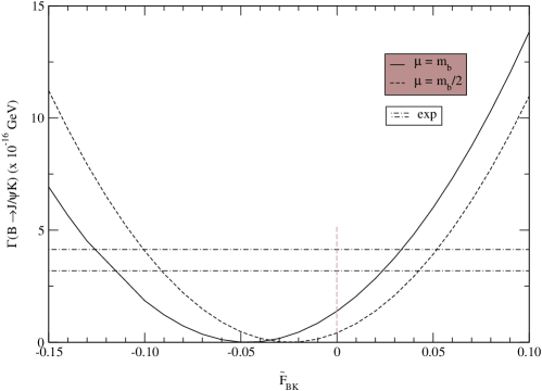
Figure 4: The partial width for $B\rightarrow J/\psi K$ as a function of the nonfactorizable amplitude $\tilde{F}_{BK}$. The dashed-dotted lines denote the experimental region.

To be able to discuss the impact of the nonfactorizable term ${\tilde{\cal O}}_{2}$, we parametrize the $\langle J/\psi K|H_{W}|B\rangle$ amplitude in terms of the $a_{2}$ parameter as

$$\langle J/\psi K|H_{W}|B\rangle=\sqrt{2}\,G_{F}\,V_{cb}V_{cs}^{*}\,\epsilon\cdot q\,m_{J/\psi}f_{J/\psi}F_{BK}^{+}(m_{J/\psi}^{2})\,a_{2}\,,$$ (29)

where

$$a_{2}=C_{2}(\mu)+\frac{C_{1}(\mu)}{3}+2C_{1}(\mu)\frac{\tilde{F}_{BK}^{+}(\mu)}{F_{BK}^{+}(m_{J/\psi}^{2})}\,.$$ (30)

The part proportional to $\tilde{F}_{BK}^{+}$ represents the contribution from the ${\tilde{\cal O}}_{2}$ operator

$$\langle J/\psi K|\tilde{\cal O}_{2}(\mu)|B\rangle=2\epsilon\cdot q\,m_{J/\psi}f_{J/\psi}\tilde{F}_{BK}^{+}(\mu^{2})$$ (31)

and $\tilde{F}_{BK}^{+}=0$ corresponds to the naive factorization result, Eq. (25).

By using the parametrization (29) we can extract the $a_{2}$ coefficient from experiments (28). The measurements yield

$$|a_{2}^{exp}|=0.29\pm 0.03\,.$$ (32)

On the other hand, the naive factorization with the NLO Wilson coefficients Buras produces

$$a_{2,\,NLO}^{fact}=0.176\,|_{\mu\simeq m_{b}}\,.$$ (33)

The value (33) is significantly below the value extracted from the experiment, although one should not forget a strong $\mu$ dependence of $a_{2}^{fact}$.

In Fig. 4 we show the partial width for $B\rightarrow J/\psi K$ as a function of the nonfactorizable amplitude $\tilde{F}_{B\rightarrow K}$. The zero value of $\tilde{F}_{BK}$ corresponds to the factorizable prediction. There exist two ways to satisfy the experimental demands on $\tilde{F}_{BK}$. Following the large $1/N_{c}$ rule BGR , one can argue that there is a cancellation between $1/N_{c}$ piece of the factorizable part and the nonfactorizable contribution (30). This would ask for the relatively small and negative value of $\tilde{F}_{BK}$. The other possibility is to have even smaller, but positive values for $\tilde{F}_{BK}$, which then compensate the overall smallness of the factorizable part and bring the theoretical estimation for $a_{2}$ in accordance with experiment.

One can note significant $\mu$ dependence of the theoretical expectation for the partial width in Fig. 4, which brings an uncertainty in the prediction for $\tilde{F}_{BK}(\mu)$ in the order of $30\%$. This uncertainty is even more pronounced for the positive solutions of $\tilde{F}_{BK}(\mu)$. The values for $\tilde{F}_{BK}^{+}$ extracted from experiments

$$\tilde{F}_{BK}^{+}(m_{b})=0.028\qquad{\rm or}\qquad\tilde{F}_{BK}^{+}(m_{b})=-0.120\,,$$ (34)

$$\tilde{F}_{BK}^{+}(m_{b}/2)=0.046\qquad{\rm or}\qquad\tilde{F}_{BK}^{+}(m_{b}/2)=-0.095\,.$$ (35)

clearly illustrate the $\mu$ sensitivity of the nonfactorizable part.

In what follows we calculate the nonfactorizable contribution $\tilde{F}_{BK}^{+}$ which appears due to the exchange of soft gluons using the QCD light-cone sum rule method.

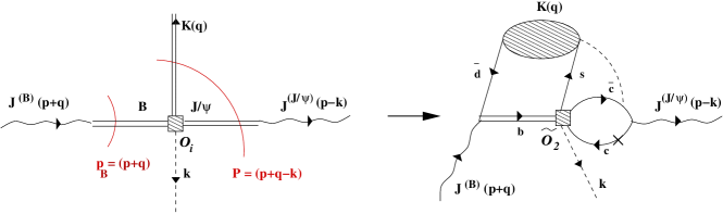
Figure 5: Sum rule calculation of the $B\rightarrow J/\psi K$ decay. The dashed line denote an exchange of a soft gluon for ${\cal O}_{i}=\tilde{\cal O}_{2}$ and the cross stands for other possible attachment of a soft gluon.

4.1 Light-Cone Sum Rule Calculation

The light-cone sum rule calculation starts by considering the correlator

$$F_{\nu}(p,q,k)=i^{2}\int d^{4}xe^{-i(p+q)x}\int d^{4}ye^{i(p-k)y}\langle K(q)|T\{J_{\nu}^{(J/\psi)}(y){\cal O}(0)J_{5}^{(B)}(x)\}|0\rangle$$ (36)

with the interpolating currents $J_{\nu}^{(J/\Psi)}=\overline{c}\gamma_{\nu}c$ and $J_{5}^{(B)}=m_{b}\overline{b}i\gamma_{5}u$. The kinematics is the same as defined above in (22), with the exception that now $p^{2}=m_{J/\psi}^{2}$. More explicitly the configuration is shown in Fig. 5.

The estimation of nonfactorizable contributions was performed for the exchange of soft gluons (shown by the dashed line in Fig. 5) and follows essentially steps of derivation explained in Sect. 3.2 for $B\rightarrow\pi\pi$ decay. Nonfactorizable contribution of the ${\cal O}_{1}$ operator appears first at $O(\alpha_{s}^{2})$. Nonvanishing result at the one-gluon level includes contribution of the $\tilde{\cal O}_{2}$ operator and the leading contributions are given in terms of twist-3 and twist-4 kaon distribution amplitudes which contribute in the same order. Technical peculiarities of the calculation can be found in mi .

4.2 Results and Implications

The results can be summarized as follows. Soft nonfactorizable twist-3 and twist-4 contributions, expressed in terms of $\tilde{F}^{+}_{BK}$ are $\tilde{F}^{+}_{BK,tw3}(\mu_{b})=0.003-0.0055$ and $\tilde{F}^{+}_{BK,tw4}(\mu_{b})=0.006-0.0012$ and the final value is

$$\tilde{F}^{+}_{BK}(\mu_{b})=0.009-0.0017\,.$$ (37)

where $\mu_{b}=\sqrt{M_{B}^{2}-m_{b}^{2}}\simeq m_{b}/2$. The wide range prediction for $\tilde{F}^{+}_{BK}$ appears due to the variation of sum rule parameters.

First, we note that the nonfactorizable contribution (37) is much smaller than the $B\rightarrow K$ transition form factor $F_{BK}^{+}=0.55\pm 0.05$, which enters the factorization prediction (26). It is also significantly smaller than the value (35) extracted from experiments. Nevertheless, its influence on the final prediction for $a_{2}$ is significant, because of the large coefficient $2C_{1}$ multiplying it. Further, one has to emphasize that $\tilde{F}_{BK}^{+}$ is a positive quantity. Therefore, we do not find a theoretical support for the large $N_{c}$ limit assumption discussed in Sect.4.1, that the factorizable part proportional to $C_{1}(\mu)/3$ should at least be partially cancelled by the nonfactorizable part. Our result also contradicts the result of the earlier application of QCD sum rules to $B\rightarrow J/\psi K$ KR3 , where negative and somewhat larger value for $\tilde{F}_{BK}^{+}$ was found. However, earlier applications of QCD sum rules to exclusive $B$ decays exhibit some deficiencies discussed in Khodja .

Using the same values for the NLO Wilson coefficients as in Sect.2, one gets from (37) the following value for the effective coefficient $a_{2}$:

$$a_{2}\sim 0.14-0.17\,|_{\mu=\mu_{b}}\,.$$ (38)

Although the soft correction contributes in the order of $\sim 30\%-70\%$, the net result (38) is still by approximately factor of two smaller than the experimentally determined value (32).

We would like to discuss our results for soft nonfactorizable contributions in comparison with the hard nonfactorizable effects calculated in the QCD-improved factorization approach. The best thing would be to calculate both soft and hard contributions inside the same model. In principle, the light-cone sum rule approach presented here enables such a calculation, although the estimation of hard nonfactorizable contributions is technically very demanding, involving a calculation of two-loop diagrams. Therefore, we proceed with the QCD-improved factorization estimations for the hard nonfactorizable contributions.

After including the hard nonfactorizable corrections, the $a_{2}$ parameter (38) is as follows

$$a_{2}=\left[C_{2}(\mu)+\frac{C_{1}(\mu)}{3}+2C_{1}(\mu)\left(\alpha_{s}F(\mu)^{hard}+\frac{\tilde{F}^{+}_{BK}(\mu)}{F^{+}_{BK}}\right)\right]\,.$$ (39)

The estimations done in the QCD-improved factorization Cheng show hard-gluon exchange corrections to the naive factorization result in the order of $\sim 25\%$, predicted by the LO calculation with the twist-2 kaon distribution amplitude. Unlikely large corrections are obtained by the inclusion of the twist-3 kaon distribution amplitude. Anyhow, due to the obvious dominance of soft contributions to the twist-3 part of the hard corrections in the BBNS approach BBNS , it is very likely that some double counting of soft effects could appear if we naively compare the results. Therefore, taking only the twist-2 hard nonfactorizable corrections from Cheng into account, recalculated at the $\mu_{b}$ scale, our prediction (38) changes to

$$a_{2}=0.16-0.19\,|_{\mu=\mu_{b}}$$ (40)

The prediction still remains too small to explain the data.

Nevertheless, there are several things which have to be stressed here in connection with the result. Soft nonfactorizable contributions are at least equally important as nonfactorizable contributions from the hard-gluon exchange, and can be even dominant. Soft nonfactorizable contributions are positive, and the same seems to be valid for hard corrections. While hard corrections have an imaginary part, in the soft contributions the annihilation and the penguin topologies as potential sources for the appearance of an imaginary part were not discussed. A comparison between the result (40) and the experimental value $|a_{2}|\sim 0.3$ for $B\rightarrow J/\psi K$ decay, with the recently deduced $a_{2}$ parameter from the color-suppressed $\overline{B}^{0}\rightarrow D^{(\ast)0}\pi^{0}$ decays, $|a_{2}|\sim 0.4-0.5$ NP , provides clear evidence for the nonuniversality of the $a_{2}$ parameter in color-suppressed decays.

5 Conclusions

We have reviewed recent progress in the understanding of the underlaying dynamics of exclusive nonleptonic decays, with the emphasis on the nonfactorizable corrections to the naive factorization approach. In the calculation of nonfactorizable contributions, we have focused to QCD light-cone sum rule approach and have shown results for $B\rightarrow\pi\pi$ Khodja and $B\rightarrow J/\psi K$ mi decays.

The QCD-improved factorization method is reviewed in this volume by M. Neubert, Neubert .

References

- (1) J. B. Bjorken: Nucl. Phys. (Proc. Suppl.) 11 321 (1989)
- (2) G. Buchalla, A.J. Buras, M.E. Lautenbacher: Rev. Mod. Phys. 68 1125 (1996)
- (3) M. Neubert: in this Volume
- (4) R. Fleisher: in this Volume
- (5) Th. Mannel: in this Volume
- (6) A. J. Buras: Nucl. Phys. B 434 606 (1995)
- (7) M. Neubert, B. Stech: Adv. Ser. Direct. High Energy Phys. 15 (1998) 294 and hep-ph/9705292
- (8) A. J. Buras, J. M. Gerard, R. Rückl: Nucl. Phys.B 268 16 (1986)
- (9) B.Y. Blok, M.A. Shifman: Sov. J. Nucl. Phys. 45 135,307,522 (1987)
- (10) M. Neubert, A. A. Petrov: Phys. Lett. B 519 50 (2001)
- (11) M. Beneke, G. Buchalla, M. Neubert, C. T. Sachrajda, Nucl. Phys. B 591 (2000) 313; Nucl. Phys. B 606 (2001) 245
- (12) Y.-Y. Keum, H.-n. Li and A.I. Sanda: Phys. Lett. B 504 6 (2001); Phys. Rev. D 63 054008 (2001)
- (13) A. Khodjamirian: Nucl. Phys. B 605 558 (2001)
- (14) E. de Rafael: ’An Introduction to Sum Rules in QCD’. In: Probing the Standard Model of Physical Interactions, ed. by R. Gupta, A. Morel, E. De Rafael, F. David (Elsevier, Amsterdam, The Netherlands 1999) and hep-ph/9802448
- (15) M. A. Shifman, A.I. Vainstein and V.I. Zakharov: Nucl. Phys. B 147 385, 448 (1979)
- (16) P. Colangelo, A. Khodjamirian: ’QCD Sum Rules, a Modern Perspective’. In: At the Frontier of Particle Physics, Vol.3, ed. M. Shifman (Singapore, World Scientific 2001) pp. 1495-1576 and hep-ph/0010175.
- (17) V.M. Braun: ’Light Cone Sum Rules’. In: Rostock 1997, Progress in Heavy Quark Physics, ed. by M. Beyer, T. Mannel, H. Schroderi (Rostock, Germany, University of Rostock 1998) pp. 105-118 and hep-ph/9801222
- (18) L.J. Reinders, H. Rubinstein: S. Yazaki: Phys. Rep. 127 1 (1985)
- (19) G.P.Lepage and S. Brodsky: Phys. Rev. D 22 2157 (1980)
- (20) B. Melić and R. Rückl: ’Nonfactorizable Effects in the Decay’, preprint WUE-ITP-2002-020
- (21) B. Aubert et al.: Phys. Rev. D 65 032001 (2002)
- (22) J. Soares: Phys. Rev. D 51 3518 (1995)
- (23) A. Khodjamirian, R. Rückl: ’Exclusive Nonleptonic Decays of Heavy Mesons in QCD’. In Continuous Advances in QCD 1998, ed. A.V. Smilga, (World Scientific, Singapore 1998), p. 287 and hep-ph/9807495.
- (24) H.-Y. Cheng, K.-Ch. Yang: Phys. Rev. D 63 074011 (2001)