Threshold effects and Planck scale Lorentz violation:
combined constraints from high energy astrophysics

Abstract

Recent work has shown that dispersion relations with Planck scale Lorentz violation can produce observable effects at energies many orders of magnitude below the Planck energy $M$. This opens a window on physics that may reveal quantum gravity phenomena. It has already constrained the possibility of Planck scale Lorentz violation, which is suggested by some approaches to quantum gravity. In this work we carry out a systematic analysis of reaction thresholds, allowing unequal deformation parameters for different particle dispersion relations. The thresholds are found to have some unusual properties compared with standard ones, such as asymmetric momenta for pair creation and upper thresholds. The results are used together with high energy observational data to determine combined constraints. We focus on the case of photons and electrons, using vacuum Čerenkov, photon decay, and photon annihilation processes to determine order unity constraints on the parameters controlling $O(E/M)$ Lorentz violation. Interesting constraints for protons (with photons or pions) are obtained even at $O((E/M)^{2})$, using the absence of vacuum Čerenkov and the observed GZK cutoff for ultra high energy cosmic rays. A strong Čerenkov limit using atmospheric PeV neutrinos is possible for $O(E/M)$ deformations provided the rate is high enough. If detected, ultra high energy cosmological neutrinos might yield limits at or even beyond $O((E/M)^{2})$.

I Introduction

The principle of relativity of motion goes all the way back to Galileo dialog , who noted that observers below decks in a large ship gliding across a calm sea have no way of determining whether they are in motion or at rest. Einstein’s special relativity, which is founded on this principle, has been spectacularly successful in accounting for phenomena involving boost factors as high as $10^{11}$. Moreover, the Lorentz group has a beautiful mathematical structure, and this symmetry powerfully constrains theories in a way that has been very useful in discovering new laws of physics. It is natural to assume under these circumstances that Lorentz invariance is a symmetry of nature up to arbitrary boosts. Nevertheless, there are several good reasons to question exact Lorentz symmetry.  From a logical point of view, the most compelling reason is that while $10^{11}$ is a large number, it is nowhere near infinity. There is, and will always be, an infinite volume of the Lorentz group that is experimentally untested since, unlike the rotation group, the Lorentz group is non-compact. Why should we assume that exact Lorentz invariance holds when this hypothesis cannot even in principle be tested?

While the non-compactness reason for questioning Lorentz symmetry is perhaps logically compelling, it is by itself not very encouraging. However, there are also several reasons to suspect that there will be a failure of Lorentz symmetry at some energy or boosts. One reason is the ultraviolet divergences of quantum field theory, which are a direct consequence of the assumption that the spectrum of field degrees of freedom is boost invariant. Another reason comes from quantum gravity. Profound difficulties associated with the “problem of time” in quantum gravity Isham ; Kuchar have suggested that an underlying preferred time may be necessary to make sense of this physics. Also tentative results in string theory KS89 , quantum geometry loopqg , and non-commutative geometry Hayakawa ; Carroll:2001ws ; Amelino-Camelia:2001cm approaches to quantum gravity have suggested that Lorentz symmetry may be broken in the ground state.

Finally, there have been recent hints from high energy astroparticle physics that we may already be seeing the effects of Lorentz violation (although as discussed below the most recent analyses make this seem unlikely.) One comes from the photo-production of electron-positron pairs when cosmic gamma rays collide with photons of the infrared background. Below 10 TeV the (indirectly) observed absorption of such gamma rays by this process offers support for boost invariance up to the boost that relates the cosmic rest frame to the center of mass frame of the colliding photons. (For a 10 TeV gamma ray colliding head on with a 25 meV infrared photon this yields a boost of $10^{7}$.) However, according to some (but not all) models of the infrared background, there appears to be less absorption than expected for gamma rays above 10 TeV coming from the blazar Mkn 501 (located at about $157$ Mpc from us). If true this could be explained by an upward threshold shift due to a Planck scale suppressed Lorentz violating term in the dispersion relation for the gamma rays Protheroe:2000hp .

The other hint comes from the cosmic ray events beyond the GZK cutoff G ; ZK on high energy protons. Ultra high energy protons undergo inelastic collisions with CMBR photons leading to the production of pions (the boost to the center of mass frame yields the figure of $10^{11}$ mentioned above). As a result, protons above $\sim 5\times 10^{19}$ eV are not able to reach us from distances above a few Mpc Stecker68 . In spite of this prediction, cosmic rays with energy beyond $10^{20}$ eV have apparently been observed by the AGASA experiment GZKdata (see also NW00 for a review on this issue). The nature and origin of these ultra high energy cosmic rays is unknown and several explanations have been proposed (see Sigl ; Stecker:2002fh for an extensive review). One proposal is that Lorentz violating terms in the dispersion relation for the proton produce an upward shift of the threshold for pion production, allowing these high energy protons to reach us Mestres ; CG ; Bertolami ; ACP . Interestingly it was argued that a universal Lorentz violating deformation of the particle dispersion relations would be capable of explaining both the TeV gamma ray absorption anomaly and the trans-GZK events ACP .

The evidence for the TeV gamma ray and GZK anomalies is not convincing at this stage, however. Indeed it has been argued in stecker01 ; Stecker:2002fh for the former and in Bahcall:2002wi ; FLYeye02 for the latter that the data are consistent with Lorentz invariance. For us therefore the most important point is just that it is possible at all that Planck scale violations of Lorentz symmetry could be observed or constrained by current and upcoming observations. The focus of the present paper is almost entirely on the constraints that can be imposed. Our work extends prior results Mestres ; CG ; Bertolami ; Acea ; ACP ; Kluzniak ; Kifune:1999ex ; Aloisio:2000cm in several ways: (i) combining constraints to limit parameter space of a priori independent parameters, (ii) discovery and characterization of the asymmetric threshold effect, (iii) characterization of upper threshold effects, (iv) extending analysis for threshold effects to higher order nonlinearities. A brief report on some of our results has already been given in Jacobson:2001tu . Some of these results have been confirmed in Major .

In the next section we discuss our theoretical framework and list the reactions we are going to consider. In Section III we study the kinematics of some photon–electron processes in order to determine how Lorentz violating dispersion affects thresholds. The details of the photon annihilation threshold analysis are worked out in the Appendix. These results are then used to deduce observational constraints on the electron and photon deformation parameters. Taken jointly these constraints severely restrict the parameter plane. Section IV is devoted to the discussion of other possible interactions including hadrons or neutrinos, and in section V we discuss the special case of common Lorentz violating parameters for all the particles. Finally we present some conclusions and perspectives in section VI.

Throughout this paper we adopt the following notational conventions: ${p_{\rm 4}}$ denotes a four-momentum ${p_{\rm 4}}=(\omega,{\mathbf{p}})$, and $p$ is the magnitude of the three-vector ${\mathbf{p}}$. The metric signature is $(+,-,-,-)$. We use the energy scale $M=10^{19}$ GeV to form dimensionless Lorentz-violating parameters, since it is close to the Planck energy $M_{\rm P}=(\hbar c^{5}/G)^{1/2}\simeq 1.22\cdot 10^{19}$ which we are presuming sets the scale for violation of Lorentz invariance induced by quantum gravity. We often employ units in which $M=1$.

II Theoretical framework and processes considered

Various approaches to quantum gravity have suggested that violations of local Poincaré symmetry might occur, but no reliable prediction is currently availble. These suggestions range from the breaking of just the boost symmetry to breaking of the full local Poincaré group. In this paper we study the former case since it is the minimal one for which consequences of boost symmetry violation can be explored. Thus we shall assume that rotation and spacetime translation symmetries are preserved, so that in particular energy and momentum are conserved.

Dispersion relations determine how particles propagate and, via energy-momentum conservation, how their interactions are kinematically constrained. Hence Lorentz violating dispersion relations provide a relatively theory-independent window into the possibility of Lorentz violating physics. In this work we explore the observational consequences of such deformed dispersion relations in flat spacetime, i.e neglecting gravitational effects. The consequences of such dispersion relations have also been extensively investigated in the context of the Hawking effect (see e.g. Jacobson:1999zk and references therein) and the primordial spectrum of density fluctuations in cosmology (see e.g. Niemeyer:2002ze ; Niemeyer:2002kh ; Brandenberger:2002sr and references therein).

In this section we discuss our framework for parametrizing such Lorentz violating physics, as well as the processes through which one might hope to place constraints or to observe Lorentz violation.

II.1 Theoretical framework

A dispersion relation that is not boost invariant can hold in only one frame. We assume this frame coincides with that of the cosmic microwave background. As mentioned above, we further assume that rotation invariance is preserved in this preferred frame. Thus the dispersion relation takes the form $E=E(p)$, where $p$ is the magnitude of ${\mathbf{p}}$. In the Lorenz invariant case we have $E^{2}=m^{2}+p^{2}$. Effective field theory suggests that it should suffice to consider generalizations of this form involving only integer powers of momentum,

$$E^{2}=m^{2}+p^{2}+\sum_{n=1}^{\infty}a_{n}p^{n}.$$ (1)

We presume that any Lorentz violation is associated with quantum gravity and suppressed by at least one inverse power of the Planck scale $M$. For $n\geq 3$ it is therefore natural to factor out the appropriate power of $M$ and write $a_{n}=\eta_{n}/M^{n-2}$ where $\eta_{n}$ is a dimensionless constant that might be expected to be of order unity if indeed quantum gravity does violate Lorentz symmetry. For $n<3$ there must in addition be another mass scale, $\mu$, which might be a particle physics mass scale, in terms of which the coefficents $a_{1,2}$ can be written as $a_{1}=\alpha_{1}\,\mu^{2}/M$ and $a_{2}=\alpha_{2}\,\mu/M$, where again $\alpha_{1,2}$ might be expected to be of order unity. In a situation such as this, the important terms at low energies $p\ll\mu$ would be from $p^{1}$ and $p^{2}$. At high energies $p\gg\mu$, the $p^{3}$ term if present would dominate. If this term is absent then the $p^{4}$ term would dominate when $p^{2}\gg\mu M$.

A large amount of both theoretical and experimental work has been done on the case $n\leq 2$. The most general framework is the “standard model extension” Kc , which includes not just rotation invariant effects but all possible renormalizable Lorentz and CPT violating terms that can be added to the standard model Lagrangian preserving the field content and gauge symmetries. Low energy observations Kc ; Kostelecky:Meeting ; Kostelecky:2001mb have placed stringent limits on the magnitude of such Lorentz and CPT violating terms. For example in Kostelecky:2001mb a very strong constraint of order $10^{-32}$ from spectropolarimetry is provided for the electromagnetic birefringence of the vacuum in the standard model extension. High energy astroparticle phenomena CG ; SG01 have also been used, however in the case of such phenomena the above discussion suggests that unless the $p^{3}$ term is absent it would be expected to dominate over the $p^{2}$ and $p^{1}$ corrections.

In this paper we focus on the constraints that can be obtained from high energy phenomena. In the absence of peculiar tuning of the coefficients of the terms with different powers $p^{n}$, it is natural to suppose that the lowest nonzero term with $n\geq 3$ will dominate at these energies. Hence, for simplicity, we shall include only one Lorentz violating power of momentum. Our study thus amounts to studying the observational consequences of dispersion relations of the form

$$E^{2}=p^{2}+m^{2}_{a}+\eta_{a}{p^{n}}/{M^{n-2}}.$$ (2)

The subscript $a$ denotes different particles, and a priori all the dimensionless coefficients $\eta_{a}$ could be different. (For notational uniformity we use here $\eta_{1,2}$ rather than the coefficients $\alpha_{1,2}$ defined above.) We assume that, in addition to being conserved, energy and momentum add for composite systems in the usual way. It might seem that the effects of such deformations of the dispersion relation could be important only near the Planck energy. However, there are at least two types of phenomena for which this is not the case.

First, for particles that propagate over cosmological distances, small differences in propagation speed can build up to detectable time-of-flight differences. Second, thresholds for particle reactions can be shifted, and thresholds can appear for normally forbidden processes. These threshold effects can occur at energies many orders of magnitude below the Planck scale. To see why, note that thresholds are determined by particle masses, hence if the $p^{n}$ term is comparable to the $m^{2}$ term in (2) one can expect a significant threshold shift. This occurs at the momentum

$$p_{\rm dev}\sim\left({m^{2}M^{n-2}/\eta}\right)^{1/n},$$ (3)

which gives a rough idea of the energies at which we expect to see deviations from standard physics. The typical scales for some different particles if $\eta\sim 1$ are summarized in Table 1.

Table 1: Typical energies at which one can expect deviations from standard kinematics for different particles if $\eta\sim 1$ and $n=3,4$. The mass of the neutrino is taken to be $\sim 1$ eV, this being the current upper bound on the mass of the lightest neutrino.

n	$p_{\rm dev}$ for $\nu_{\rm e}$	$p_{\rm dev}$ for $e^{-}$	$p_{\rm dev}$ for $p^{+}$
3	$\sim 1$ GeV	$\sim 10$ TeV	$\sim 1$ PeV
4	$\sim 100$ TeV	$\sim 100$ PeV	$\sim 3$ EeV

II.2 Viability of theoretical framework

Before considering the observational constraints, a few comments are in order regarding the viability of the theoretical framework we are adopting.

• Restriction to $p\ll M$ and monotonicity of $E(p)$
  We view the dispersion relation just as the initial terms in a derivative expansion, so we are assuming nothing about the actual Planck scale physics. In particular, when $n>2$ and $\eta$ is negative, the right hand side of the dispersion relation (2) becomes negative for large enough momenta $\sim|\eta|^{-1/(n-2)}M$. However, we never use the dispersion relation in this regime where the energy would be imaginary. Moreover, it will be important for our threshold analysis that we restrict attention even further to the regime in which the dispersion relation is strictly monotonic. As long as $|\eta|$ is not much larger than unity this will be the case provided the momentum is below the Planck scale. In fact, we consider only momenta many orders of magnitude below the Planck scale.

• Causality and stability
  For positive $\eta$ the propagation is superluminal at high energies. One might worry that this would lead to causal paradoxes, however this is not the case, since the propagation is always forward in time relative to the preferred frame in which the dispersion relation is specified. For negative $\eta$ the 4-momentum is spacelike at high energy, hence in a boosted frame the energy can be less than zero. One might think this implies that the case with $\eta<0$ is not energetically stable and hence unviable. This is not so, however, since all energies remain positive relative to the preferred frame, which is enough to guarantee stability.

• Dispersion relations for macroscopic systems
  The deformed dispersion relations are introduced for elementary particles only; those for macroscopic objects are then inferred by addition. For example, if $N$ particles with momentum ${\mathbf{p}}$ and mass $m$ are combined, the total energy, momentum and mass are $E_{\rm tot}=NE(p)$, ${\bf P}_{\rm tot}=N{\mathbf{p}}$, and $M_{\rm tot}=Nm$, so that $E_{\rm tot}^{2}=M_{\rm tot}^{2}+P_{\rm tot}^{2}+N^{2-n}\eta P_{\rm tot}^{n}$ (in units with $M=1$). The ratio of the Lorentz violating term to the $P^{2}$ term is the same as it is for the individual particles, $\eta p^{n-2}$, hence there is no observational conflict with standard dispersion relations for macroscopic objects.

• Effective field theory and compatibility with general relativity
  There is no difficulty exporting deformed dispersion relations to curved spacetime, provided they can be produced by an effective Lagrangian for a field. In this case, the preferred frame in which the dispersion relation holds is specified by a unit timelike vector field, which must be promoted to a dynamical field of the theory if general covariance is to be preserved Kostelecky:1989jw ; Carroll:vb ; Gasperini ; JM . In the cases that $n$ is even, there are obvious Lagrangians that produce the dispersion relation. For example one can add terms involving extra powers of the spatial Laplacian, such as $({}^{(3)}{\nabla}^{2}\phi)^{2}$ for a scalar field. For odd $n$ there seems to be no local action that will work for real scalar fields, although for a complex scalar the term $i\bar{\phi}\partial_{t}{}^{(3)}{\nabla}^{2}\phi+{\rm h.c.}$ induces cubic and higher order terms. To induce cubic terms for spinors one can write for example $\bar{\psi}{}^{(3)}{\nabla}^{2}\psi$, and for the electromagnetic field one can write ${\bf B}\cdot{\bf\nabla}\times{\bf E}$ (which violates parity). This last case yields a sort of Lorentz violation that emerges from quantum geometry calculations loopqg . The Lorentz violating terms in the effective Lagrangians just discussed have mass dimension greater than four so are not renormalizable. This is not a fundamental problem, since we only regard the Lagrangian as an effective one below some large energy scale, however it raises the question of naturalness. For now we take the point of view that there may be an explanation for the low energy Lorentz symmetry that is not yet understood.

II.3 Processes considered

In order to determine the strongest joint constraints on the a priori independent coefficients $\eta_{a}$ in (2) one must identify several processes involving the same types of particles. We focus most of our attention on the case of photons and electrons, since the electron mass is light and these particles interact readily. In this way we are able to obtain rather strong constraints on the allowed parameter space. We also consider several other processes some of which presently allow or will soon allow further interesting constraints to be placed. Here we summarize all the processes to be considered in the paper and a few more.

1. Photon–electron processes

   1. QED vertex interactions: The basic QED vertex involves one photon and two electron lines. With all particles on-shell this vertex is forbidden (for any in-state) by energy momentum conservation in the usual Lorentz invariant theory, but it can be allowed by Lorentz violating dispersion. In particular we consider the following processes:

      1. $e^{-}\rightarrow e^{-}\,\gamma$: This vacuum Čerenkov effect is extremely efficient, leading to an energy loss rate that goes like $E^{2}$ well above threshold. Thus any electron known to propagate must lie below the threshold. We shall also discuss the vacuum Čerenkov effect for other charged particles and even for neutral particles.

      2. $\gamma\rightarrow e^{+}\,e^{-}$: The photon decay rate goes like $E$ above threshold, so any gamma ray which propagates over macroscopic distances must have energy below the threshold.

      3. $e^{+}\,e^{-}\rightarrow\gamma$ Pair annihilation to a single photon can also occur. For cosmological observations this would be hardly distinguishable from the similar two-photon pair annihilation and as such it is not presently helpful in providing observational constraints.

   2. $\gamma\,\gamma\rightarrow e^{+}\,e^{-}$: Photon annihilation occurs in ordinary QED above a certain threshold, however Lorentz violating dispersion can modify this threshold in observationally interesting ways and can introduce an upper threshold. (The related reactions of pair annihilation (into two photons) and Compton scattering are also modified, however these effects offer no clear signal that can provide useful constraints.)

   3. $\gamma\rightarrow N\gamma$: Photon splitting is allowed by energy momentum conservation in Lorentz invariant QED if all $N+1$ photons have parallel momenta, but the process does not occur both because the matrix element vanishes and the phase space volume vanishes. With modified dispersion the photon four-momenta are no longer null (and there may be additional Lorentz violating operators that mediate the process) hence this reaction can occur with a finite rate. However, we shall see that the rate is too small to be observable.

   4. Time of flight constraints: Non-linearity in the modified dispersion relation leads to different times of arrival for photons of different wavelength emitted from the same event. Such differences can provide an upper bound on the parameter governing the amount of Lorentz violation for photons, independently of the parameters for other particles.

   5. Vacuum birefringence constraints. Violations of Lorentz invariance involving also parity violation can lead to unequal speeds of propagation for different photon polarizations. The absence of such birefringence effects for light (IR-UV) from cosmological sources has been used to provide constraints of order $10^{-32}$ and $10^{-5}$ for the quadratic Kostelecky:2001mb and cubic deformations Gleiser:2001rm respectively.

2. Other processes:

   1. Alternative vacuum Čerenkov effects

      • $p^{+}\rightarrow p^{+}\,\gamma$ or $n\rightarrow n\,\gamma$: Note that to properly analyze this reaction the structure of the proton or neutron must be taken into account.

      • $\nu\rightarrow\nu\,\gamma$: Although neutrinos are neutral, they still have a charge structure in the standard model so can in principle produce vacuum Čerenkov radiation via the charge radius coupling. Massive neutrinos could also radiate via the magnetic moment coupling Rabi . The related process of photon decay to neutrinos, $\gamma\rightarrow\bar{\nu}\nu$, may also provide an interesting constraint.

      • Gravitational Čerenkov radiation will occur if matter moves faster than the phase velocity of gravitons in vacuum Bassett:2000wj . This effect has been used, in the special case $n=2$, to place limits on the difference between the maximum speeds of propagation for gravitons and photons Moore:2001bv .

   2. $p^{+}\,\gamma_{\rm CMB}\to p^{+}\,\pi_{0}$: GZK interaction. Lorentz violations can change the allowed range of energies for this reaction. The confirmation of the standard GZK cutoff can therefore provide interesting constraints even in the case $n=4$ due to the tremendously high energy of the most energetic cosmic rays. Moreover the highest energy events recorded by AGASA may conceivably be explained via an upper threshold.

   3. Neutron stability–Proton instability. If the dispersion relations for the neutron and proton are independently modified, it is possible to make neutrons stable at high energies. The highest energy AGASA events could be understood in this manner if the trans-GZK particles were actually neutrons, hence suppressing their interaction with the cosmic background radiation.

   4. Neutrino oscillations. Non flavor-diagonal Lorentz violations can produce neutrino oscillations, even for massless neutrinos CGne . For quadratic deviations in the dispersion relation ($n=2$) the constraints from current observation have been considered in CG ; CGne ; Pak leading to a constraint on the difference of speed between electron and muon neutrinos of about $10^{-22}$. Constraints for higher order Lorentz violations have been discussed in Brustein .

   5. Anisotropy effects. The motion of the laboratory with respect to the preferred frame can produce anisotropic effects. Limits for the case $n=2$ are discussed in Kostelecky:Meeting . Such an effect has recently been used Sudarsky to show that the Lorentz violation suggested by quantum geometry calculations is in conflict with current observations in Hughes–Drever type experiments.

II.4 Observations

To obtain constraints from these reactions we shall consider the following observations:

1. Electrons of energy up to $\sim 100$ TeV are inferred via X-ray synchrotron radiation coming from supernova remnants Koyama ; Naito .

2. Gamma rays up to $\sim 50$ TeV arrive on earth from the Crab nebula Tanimori .

3. Cosmic gamma rays are absorbed in a manner consistent with photon annihilation off the IR background with the standard threshold stecker01 ; Stecker:2002fh . This inference depends on incomplete knowledge of the IR background and on assumed properties of the source spectrum however, so the consistency provides only an imprecise constraint at present.

4. Different photons emitted by the same gamma ray burst all arrive at earth within a narrow time interval.

5. The GZK cut off on UHE cosmic ray protons at $\sim 5\cdot 10^{19}$ eV has been observed Bahcall:2002wi ; FLYeye02 (although events at higher energy may have been detected GZKdata ).

Using the electron–photon processes we find strong constraints on the allowable range for the photon and electron parameters for cubic order ($n=3$) Lorentz violation, while the quartic case ($n=4$) is only weakly constrained. Using UHE cosmic ray protons we obtain strong constraints even for $n=4$.

III Photon–electron processes

In this section we determine the thresholds for some elementary processes involving just photons and electrons. The fact that these always involve the same particles will allow us to combine the constraints provided by the available observations and to severely restrict the space of the Lorentz violating parameters.  From here on we adopt units with $M=1$, but occasionally display the $M$ dependence explicitly.

III.1 Kinematics of the basic QED vertex

The processes $e^{-}\rightarrow e^{-}\gamma$ and $\gamma\rightarrow e^{+}e^{-}$ correspond to the basic QED vertex, but are normally forbidden by energy-momentum conservation together with the standard dispersion relations. When the latter are modified, these processes can be allowed.

For photons and electrons the assumed dispersion relations are:

$$\omega^{2}(k) = k^{2}+\xi k^{n},$$ (4)

$$E^{2}(p) = m^{2}+p^{2}+\eta p^{n},$$ (5)

where we have introduced the notation $\xi=\eta_{\gamma}$ and $\eta=\eta_{e}$. Let us denote the photon 4-momentum by $k_{4}=(\omega_{k},{\mathbf{k}})$, and the electron and positron 4-momenta by $p_{4}=(E_{p},{\mathbf{p}})$ and $q_{4}=(E_{q},{\mathbf{q}})$. For the two reactions energy-momentum conservation then implies $p_{4}=k_{4}+q_{4}$ and $k_{4}=p_{4}+q_{4}$ respectively. In both cases, we have

$$(p_{4}-k_{4})^{2}=q_{4}^{2},$$ (6)

where the superscript “2” indicates the Minkowski squared norm. Using the Lorentz dispersion relations (4) and (5) this becomes

$$\xi k^{n}+\eta p^{n}-\eta q^{n}=2\left(E_{p}\omega_{k}-pk\cos\theta\right),$$ (7)

where $\theta$ is the angle between ${\mathbf{p}}$ and ${\mathbf{k}}$. In the standard case the coefficients $\xi$ and $\eta$ are zero and the r.h.s. of Eq. (7) is always positive, hence there is no solution. It is clear that non-zero $\xi$ and $\eta$ can change this conclusion and allow these processes.

We define a lower threshold as the minimum energy required for the incoming particle for the reaction to occur. (If the initial state is a two particle state, then a threshold is defined relative to a fixed energy for the “target” particle. Conversely, an upper threshold is defined as the maximum energy (if any) allowed for the incoming particle for the reaction to occur. Our analysis is based on properties of thresholds summarized in the following threshold theorem:

Threshold theorem: If $E_{p}$ is a strictly monotonically increasing function of $p$ for $p>0$ for all particles, then all thresholds for processes with two particle final states occur when the final momenta are parallel. For processes with two particle initial states the initial momenta at threshold are anti-parallel.

A detailed proof can be found in JLMth . According to the theorem, $\theta=0$ at a threshold. This point has been assumed in previous work but was not shown explicitly and in fact is not true if $E_{p}$ is not monotonic.

Fixing $\theta$ to be zero, all three spatial momenta are parallel, hence momentum conservation implies $q=|{\mathbf{q}}|=|\pm({\mathbf{p}}-{\mathbf{k}})|=|p-k|$. In this case the relation (7) becomes

$$\xi k^{n}+\eta p^{n}-\eta|p-k|^{n}=2pk\left(\frac{E_{p}}{p}\frac{\omega}{k}-1\right).$$ (8)

In the situations of interest to us, the momentum $p$ is relativistic, and the Lorentz violating terms are small:

$$m/p\ll 1$$ (9)

$$\xi(k/M)^{n-2}\ll 1$$ (10)

$$\eta(p/M)^{n-2}\ll 1$$ (11)

Using these approximations and expanding the two energies in powers of the small quantities $((m/p)^{2}+\eta p^{(n-2)})$ and $\xi k^{(n-2)}$ we obtain

$$\frac{E_{p}}{p}\frac{\omega}{k}=\left[1+\frac{1}{2}\left(\frac{m^{2}}{p^{2}}+\eta p^{(n-2)}\right)-\frac{1}{8}\left(\frac{m^{2}}{p^{2}}+\eta p^{(n-2)}\right)^{2}\right]\cdot\left[1+\frac{1}{2}\xi k^{(n-2)}-\frac{1}{8}\left(\xi k^{(n-2)}\right)^{2}\right].$$ (12)

There is a subtlety about the truncation of this double expansion. If the ratio of the two expansion parameters is very large, it is possible that the second order term in one quantity is comparable to (or larger than) the first order term in the other quantity. In such cases, spurious results can be obtained by truncating both expansions at the same order. We shall proceed with the first order truncation of both expansions. One can check a posteriori whether the truncation is consistent. It turns out that this truncation is adequate for our practical purposes. In particular, although at very high energies our approximate threshold results will fail to be accurate, those energies are sufficiently high so as to be observationally irrelevant.

Another important point is that Eq. (8) originated from (6) together with conservation of three-momentum and hence it is equivalent to energy conservation $E(p)-\omega(k)=\pm E(q)$. For the Čerenkov and photon decay processes $e^{-}\rightarrow e^{-}\gamma$ and $\gamma\rightarrow e^{+}e^{-}$ we want only the upper and lower signs respectively, since the energy of all the particles should be positive. It will be unnecessary to impose this choice explicitly however, since the negative energy solutions are excluded by the approximations to be employed, as can be checked by just imposing energy conservation directly and using the same approximations. We indicate below how the approximations can exclude the negative energy solutions.

Consider for example the vacuum Čerenkov process. Then energy conservation with a negative energy final electron reads $E(p)=\omega(k)-E(q)$ with $\omega(k)$, $E(p)$ and $E(q)$ all positive. The smallest $E(q)$ can be (within the monotonic regime) is $m$, so we must have $\omega(k)>E(p)+m$. Expanding, this becomes $k+\xi k^{(n-1)}/2>p+m^{2}/2p+\eta p^{(n-1)}/2+m$. On the other hand, momentum conservation (in the threshold configuration) requires that $k<p$. This inequality implies that $\xi k^{(n-1)}/2>\eta p^{(n-1)}/2+m$, which requires that either $\xi k^{(n-2)}\gtrsim O(m/p)$, or $|\eta p^{(n-2)}|\sim m/p$, or both. In either case, we see that neglected terms such as $(\xi k^{(n-2)})^{2}$ are not negligible compared to the term $(m/p)^{2}$ that has been kept.

Truncating (12) at first order, and inserting the result in Eq. (8) we obtain

$$\xi k^{n}+\eta p^{n}-\eta|p-k|^{n}=2pk\left(\frac{m^{2}}{2p^{2}}+\frac{\xi}{2}k^{(n-2)}+\frac{\eta}{2}p^{(n-2)}\right).$$ (13)

Introducing the variable $x=k/p$, (13) takes the form

$$\frac{m^{2}}{p^{n}}=-\xi x^{(n-2)}\left(1-x\right)+\eta\left[\frac{1-x-|1-x|^{n}}{x}\right].$$ (14)

At threshold for either Čerenkov or photon decay $p$ and $x$ must satisfy this kinematic relation. Note that while we have assumed that $p$ is relativistic, no such assumption is needed for the other two momenta $q$ and $k$. This is important since we shall use (14) in cases where the momentum distribution is highly asymmetric.

III.2 Vacuum Čerenkov effect: $e^{-}\to\gamma\,e^{-}$

The spontaneous emission of photons by a charged particle in vacuum is forbidden in Lorentz invariant physics since the sum of a timelike and null 4-momentum vectors cannot lie on the same mass shell as the timelike 4-momentum. Modifications of the dispersion relations of the form (4) and (5) can allow some phase space for this reaction to happen. If the reaction is allowed the rate of energy loss for the case $n>2$ well above threshold is $dE/dt\sim\alpha E^{2}$, where $E$ is the energy of the initial charged particle and $\alpha$ is the fine structure constant. The decay distance is thus only of order the microscopic distance $100/E$, hence the lower threshold of the vacuum Čerenkov effect must be above the maximal observed energy of any charged particle known to propagate.

The lower threshold is the lowest value of the incoming electron momentum $p$ for which the kinematic equation (14) has a solution. At threshold $x=k/p$ must lie between 0 and 1, since if $k$ were greater than $p$ the final electron momentum would have to be anti-parallel to the photon momentum, which is excluded by the threshold theorem (cf. Sect. III.1). The threshold therefore occurs at the value of $x$ in this range for which the right hand side has a maximum. We substitute this $x$ in Eq (14) to obtain the lower threshold momentum for the electron as a function of $\xi,\eta$ and $m$. That there is no upper threshold in this case is immediately obvious since the right hand side vanishes as $x$ approaches one, allowing solutions with arbitrarily large momentum.

The analysis is somewhat simplified by rewriting Eq. (14) in terms of the new variable $w=1-x$, in terms of which it takes the form

$$\frac{m^{2}}{p^{n}}=-\xi w(1-w)^{n-2}+\eta(w+\cdots+w^{n-1}).$$ (15)

The relevant range of $w$ is 0 to 1. In the threshold configuration we have $p=q+k$, hence $w=q/p$. The general analysis of the threshold relations must be done on a case by case basis for different values of $n$, however it is easy to derive partial results valid for any $n$.

First consider the case where $\xi$ is positive. Then the first term in (15) is negative, so if $\eta$ is negative there is no solution. If $\eta$ is positive, the maximum of the right hand side clearly occurs at $w=1$, where it is equal to $(n-1)\eta$. Hence the threshold for the case when $\xi$ and $\eta$ are both positive and $n>2$ is

$$p_{\rm th}=\left[\frac{m^{2}}{(n-1)\eta}\right]^{1/n}.$$ (16)

Since $w=1$, this threshold corresponds to the emission of a zero energy photon. This is why the value of $\xi$ is irrelevant, and the Čerenkov process takes place as long as $\eta$ is positive. Indeed also for negative values of $\xi$ the process takes place as long as $\eta$ is positive (and even for some negative values—see below), however the threshold configuration may occur with the emission of a hard photon.

One more general result can be established, namely that there is no threshold if $\eta\leq\xi\leq 0$. To see this observe that for $w$ between 0 and 1 we have $w+\cdots+w^{n-2}>w(1-w)^{n-2}$, since the derivative of the lhs is greater than unity and the derivative of the rhs is less than unity. Thus if $\eta\leq\xi\leq 0$ the rhs of (15) is nowhere positive in this range of $w$. In particular, there is no threshold in the case of equal negative parameters $\xi=\eta<0$.

The remaining parameter space for which we need to determine the threshold is the region $\xi<0$ and $\eta>\xi$.

III.2.1 Vacuum Čerenkov thresholds for $n=2,3,4$

In the case $n=2$ equation (15) becomes

$$\frac{m^{2}}{p^{2}}=(\eta-\xi)w,$$ (17)

hence the threshold occurs at $w=1$, with the emission of a zero energy photon, and the threshold momentum is given by

$$p_{\rm th}=\left(\frac{m^{2}}{\eta-\xi}\right)^{1/2}.$$ (18)

It is clear from the above expression that no threshold exists for the special case $\xi=\eta$. This can also be seen directly from the fact that quadratic modifications in the dispersion relations are equivalent to constant (momentum independent) shifts in the speed of propagation. In the case of equal coefficients the electron and photon dispersion relations share the same Lorentz symmetry only with a modified speed of light, and hence the vacuum Čerenkov effect (as well as photon decay) cannot take place. Nevertheless we shall see that in the higher order cases ($n\geq 3$) these processes are allowed for equal positive coefficients.

In the case $n=3$ equation (15) becomes

$$\frac{m^{2}}{p^{3}}=(\eta-\xi)w+(\eta+\xi)w^{2}.$$ (19)

The form of the threshold relation for $p$ depends on the values of $\eta$ and $\xi$. We find two different formulae, depending on whether the threshold occurs with emission of a low energy photon ($w\to 1$) — which we label as case a) below — or with emission of a photon with energy of order $p$ — which is labeled case b). After a bit of calculation we find:

$${\rm a)} \quad p_{\rm th}=\left(\displaystyle{\frac{m^{2}}{2\,\eta}}\right)^{1/3}\qquad\qquad\quad\>\>\>\mbox{for $\eta>0$ and $\xi\geq-3\eta$},$$ (20)

$${\rm b)} \quad p_{\rm th}=\left[\displaystyle{-\frac{4\,m^{2}\left(\xi+\eta\right)}{\left(\xi-\eta\right)^{2}}}\right]^{1/3}\quad\;\mbox{for $\xi<-3\eta<0$ or $\xi<\eta\leq 0$}$$ (21)

$${\rm c)} \quad\mbox{No threshold}\qquad\qquad\qquad\quad\mbox{for $\eta<0$ and $\xi>\eta$}.$$ (22)

In case b) the value of $w=q/p$ at the threshold is given by $q/p=-(\eta-\xi)/2(\eta+\xi)$. Given a maximal energy/momentum $p_{\rm max}$ for which no vacuum Čerenkov effect is observed, the constraint on the parameters can be written as:

$${\rm a)}\quad\eta < \displaystyle{\frac{m^{2}}{2p_{\rm max}^{3}}},$$ (23)

$${\rm b)}\quad\xi > \displaystyle{\eta-2\,\frac{m^{2}}{p_{\rm max}^{3}}-2\sqrt{\left(\frac{m^{2}}{p_{\rm max}^{3}}\right)^{2}-2\eta\left(\frac{m^{2}}{p_{\rm max}^{3}}\right)}}.$$ (24)

The case in which the correction is of quartic order is similar to the cubic one, although somewhat more complicated. In the case $n=4$ equation (15) becomes

$$\frac{m^{2}}{p^{4}}=(\eta-\xi)w+(\eta+2\xi)w^{2}+(\eta-\xi)w^{3}.$$ (25)

With the definitions $\lambda\equiv\eta-\xi$ and $\tau\equiv(\eta+2\xi)/\lambda$, (25) takes the form $m^{2}/p^{4}=\lambda(w+\tau w^{2}+w^{3})$, which is what we used to carry out the threshold analysis. Again the form of the threshold relation for $p$ depends on the values of $\eta$ and $\xi$, and we label the cases with a) and b) as for $n=3$. After some tiresome analysis we obtain the following expressions:

$${\rm a)} \quad p_{\rm th}=\left(\frac{m^{2}}{3\,\eta}\right)^{1/4}\qquad\>\>\>\,\mbox{for $\eta>0$ and $\xi\geq-(8+6\sqrt{2})\eta$},$$ (26)

$${\rm b)} \quad p_{\rm th}=\left(\frac{m^{2}}{F(\lambda,\tau)}\right)^{1/4}\quad\mbox{for $\xi<-(8+6\sqrt{2})\eta<0$ or $\xi<\eta\leq 0$},$$ (27)

$${\rm c)} \quad\mbox{No threshold}\qquad\>\>\mbox{for $\eta<0$ and $\xi>\eta$},$$ (28)

where the function $F(\lambda,\tau)$ is given by

$$F(\lambda,\tau)=\frac{2}{27}\lambda\left[\tau^{3}+\left(\tau^{2}-3\right)^{3/2}-\frac{9}{2}\tau\right].$$ (29)

In the case a) we have again the emission of a low energy photon ($w\to 1$). In case b) the value of $w=q/p$ at the threshold is given by $q/p=(-\tau-\sqrt{\tau^{2}-3})/3$. So for $n=4$ given a maximal energy/momentum (say $p_{\rm max}$) for which no vacuum Čerenkov effect is observed, the constraint for case a) can be written as:

$${\rm a)}\quad\eta<\displaystyle{\frac{m^{2}}{3p_{\rm max}^{4}}}.$$ (30)

The constraint for case b) has a cumbersome form but the corresponding line in the $\xi$–$\eta$ plane can be found from equation (27).

III.2.2 Observations and constraints from absence of vacuum Čerenkov effect

We can now consider the actual constraints observations impose on $\xi$ and $\eta$. The previous analysis shows that the smallness of $m^{2}/p_{max}^{n}$ determines the strength of the constraint provided by the vacuum Čerenkov effect, hence the strongest constraint will be obtained by considering the highest energy observed for a given particle.

Electrons in particle accelerators are stable against the vacuum Čerenkov effect at energies up to $500$ GeV, and in cosmic rays energies of $\sim 2$ TeV have been detected Kifune:1999ex ; nishi . Even higher energies, in the range $50-100$ TeV, are necessary in order to consistently explain the peaks in the X-ray and TeV regions of the photon emission from supernova remnants such as SNR1006 or the Crab Nebula Koyama ; AAK ; Kifune:1999ex . In particular for the Supernova remnant SN1006 a clear identification of a synchrotron emission together with the independent estimate of the magnetic field strength allows one to infer that the electrons should have energies of about 100 TeV Koyama ; Naito .. These electrons propagate over distances far longer than that required by the vacuum Čerenkov effect to decrease the electron energy below the threshold.

For $n=2$ we see from Eq. (18) that $(\eta-\xi)\lesssim 3\times 10^{-17}$ which can be compared with the limit $(\eta-\xi)\lesssim 5\times 10^{-13}$ obtained by Coleman and Glashow CG using a $p_{max}$ of 500 GeV. The Čerenkov emission rate (cf footnote 5) is fast enough for such parameters that $\Delta E\sim E$ over a distance scale of centimeters. For $n\geq 3$ the emission rate is $10^{17}$ times higher. For the cases of $n=3$ and $n=4$ the corresponding value of $m^{2}/p^{n}_{max}$ is $\sim 3\times 10^{-3}$ and $\sim 4\times 10^{11}$ respectively. We therefore obtain an interesting constraint for the cubic case but not for the quartic case, assuming that the Lorentz violation is at the Planck scale. (We shall see in section IV.1.1 that one could get a good constraint even for the $n=4$ case by considering the $10^{20}$ eV cosmic ray protons, modulo some caveats that we shall discuss.) Figure 1 shows the excluded region for the parameters $\xi$ and $\eta$ in the $n=3$ case as determined by the conditions (23) and (24).

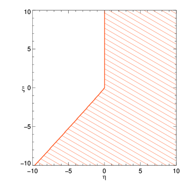
Figure 1: Constraint from the absence of vacuum Čerenkov effect for $n=3$. The filled region in the parameter space is the one not compatible with the existence of the $\sim 100$ TeV electrons indirectly detected via synchrotron emission from supernova remnants Koyama . The point where the vertical line crosses the $\eta$ axis is $\eta=m^{2}/(2p^{3}_{\rm max})\sim 1.5\times 10^{-3}$.

III.3 Photon Decay: $\gamma\to e^{+}\,e^{-}$

The spontaneous decay of a photon into a electron-positron pair, is another reaction usually forbidden by energy–momentum conservation. As in the case of the vacuum Čerenkov effect, modifications of the dispersion relation allow this reaction to occur. By the threshold theorem (cf. Sect. III.1), we know that the final particles have parallel momenta, so that both lepton momenta are less than or equal to $k$. Thus $x:=k/p\geq 1$ in Eq. (14), so that $|1-x|=x-1$. It is convenient to use the variable $y:=1/x=p/k$, whose relevant range is zero to one. In terms of y, (14) takes the form

$$\frac{m^{2}}{k^{n}}=\xi y\left(1-y\right)-\eta y\left(1-y\right)\left[y^{(n-1)}+\left(1-y\right)^{(n-1)}\right].$$ (31)

The threshold corresponds to the maximum of the right hand side of Eq. (31) with respect to $y$. Note that the rhs is symmetric about $y=1/2$, since the two leptons are kinematically interchangeable, hence it is always stationary at $y=1/2$. However, this stationary point can be a maximum or a minimum, depending on the values of $\eta$ and $\xi$. If it is a maximum the threshold momentum is given by

$$k_{\rm th}=\left[\frac{2^{n}m^{2}}{2^{(n-2)}\xi-\eta}\right]^{1/n}.$$ (32)

In the special case $\xi=\eta$, which has been mostly studied in the literature, it can be shown that the only stationary points of (31) are $y=0,1/2,1$. Given that the right hand side of Eq. (31) is always zero at $y=0,1$ it follows that for equal coefficients the threshold condition is always realized with a symmetric distribution of the final momenta.

Contrary to relativistic intuition, and to what has been assumed in all previous calculations as far as we know, the threshold does not always occur with the symmetric configuration. The reason is that when $\eta<0$, the lepton energy $E(p)$ has negative curvature $E^{\prime\prime}(p)<0$ for sufficiently large momentum if $n>2$, unlike the usual Lorentz invariant case. If the threshold lies within the negative curvature region, it cannot occur with the symmetric configuration since the energy of the final state at fixed momentum could be lowered by making the momentum of one particle smaller and one larger by an equal amount. For $\eta<\xi<0$, the threshold does occur in the negative curvature region, hence it is asymmetric.

The occurrence of the asymmetric threshold might seem especially surprising if we think, with relativistic habits, that at threshold the electron and positron should be created at rest in the center of mass frame. The error lies in a misleading application of the Lorentz transformation in the case where a definite preferred system exists. First, the center of mass frame may not even be accessible if the photon energy-momentum vector is spacelike (i.e. subluminal dispersion). Second, even if we can boost to the center of mass frame, in this frame the dispersion relation of the electron/positron may not have its minimum energy at zero momentum. Therefore it is not always true that the final particles are produced at rest in the center of mass frame.

We now examine the cases $n=2,3,4$ individually.

III.3.1 Photon decay thresholds for $n=2,3,4$

In the case $n=2$ Eq. (31) takes the form

$$\frac{m^{2}}{k^{2}}=(\xi-\eta)y(1-y).$$ (33)

For $\xi-\eta<0$ there is no threshold, while for $\xi-\eta>0$ there is a lower threshold at $y=1/2$. In this case one obtains the threshold formula

$$k_{\rm th}=\frac{2m}{\sqrt{\xi-\eta}}$$ (34)

In the case $n=3$ (31) takes the form

$$\frac{m^{2}}{k^{3}}=\xi y\left(1-y\right)-\eta y\left(1-y\right)\left[y^{2}+\left(1-y\right)^{2}\right],$$ (35)

To determine the threshold we need to find the maximal values of the rhs. The task of finding the maxima is simplified by introducing the new variable $z=(2y-1)^{2}$, so that $y=(1+\sqrt{z})/2$, $(1-y)=(1-\sqrt{z})/2$, and $y(1-y)=(1-z)/4$. The relevant range of $z$ is $[0,1]$, where $z=0$ corresponds to the symmetric configuration $y=1/2$ and $z=1$ corresponds to $y=1$.

In terms of $z$, (35) becomes

$$\frac{m^{2}}{k^{3}}=\frac{\xi}{4}(1-z)-\frac{\eta}{8}(1-z^{2})$$ (36)

The symmetric extremum at $y=1/2$ corresponds to $z=0$, and there is one other (asymmetric) extremum at $z_{a}=\xi/\eta$. One of the two extrema is a maximum and the other is a minimum. Since the second derivative with respect to $z$ is $\eta/4$, the one at $z_{a}$ is a maximum  if and only if $\eta<0$, and it lies between zero and one in this case if and only if $\eta<\xi<0$. Note that in the special case $\xi=\eta$ the asymmetric threshold solution is removed and a threshold exists just for positive values of $\eta$.

The value of the rhs of (36) at $z=0$ is $(2\xi-\eta)/8$, while at $z=z_{a}$ it is $-(\xi-\eta)^{2}/8\eta$. We thus see that photon decay is allowed only above the broken line in the $\eta$–$\xi$ plane given by $\xi=\eta/2$ in the quadrant $\xi,\eta>0$ and by $\xi=\eta$ in the quadrant $\xi,\eta<0$. Above this line, the threshold is given by

$$\mbox{a)}\quad k_{\rm th} = \displaystyle{\left(\frac{8m^{2}}{2\xi-\eta}\right)^{1/3}}\quad\mbox{for $\xi\geq 0$},$$ (37)

$$\mbox{b)}\quad k_{\rm th} = \displaystyle{\left[\frac{-8m^{2}\eta}{\left(\xi-\eta\right)^{2}}\right]^{1/3}}\quad\mbox{for $\eta<\xi<0$}.$$ (38)

The detection of gamma rays with momenta up to some $k_{\rm max}$ implies that the parameters must lie in the $\xi-\eta$ plane below the line corresponding to a threshold at $k_{\rm max}$. This translates into the following constraints for the parameters $\xi$ and $\eta$

$$\mbox{a)}\quad\xi<\displaystyle{\frac{\eta}{2}+\frac{4m^{2}}{k^{3}_{\rm max}}},\qquad\mbox{b)}\quad\xi<\displaystyle{\eta+\sqrt{-\frac{8m^{2}\eta}{k^{3}_{\rm max}}}}.$$ (39)

In the case $n=4$ Eq. (31) can again be conveniently rewritten in terms of the variable $z$ introduced after (35) above, yielding

$$\frac{m^{2}}{k^{4}}=\frac{\xi}{4}(1-z)-\frac{\eta}{16}(1+2z-3z^{2}).$$ (40)

The asymmetric extremum here occurs at $z_{a}=(2\xi+\eta)/3\eta$. This is again a maximum if and only if $\eta<0$, and it lies between zero and one in this case if and only if $\eta<\xi<-\eta/2$. Note that again in the special case $\xi=\eta$ the asymmetric threshold solution is removed and a threshold exists just for positive values of $\eta$.

The value of the rhs of of (40) at $z=0$ is $(4\xi-\eta)/16$, while at $z=z_{a}$ it is $-(\xi-\eta)^{2}/12\eta$. We thus see that photon decay is allowed only above the broken line in the $\eta$–$\xi$ plane given by $\xi=\eta/4$ in the quadrant $\xi,\eta>0$ and by $\xi=\eta$ in the $\xi,\eta<0$. Above this line, the threshold is given by

$$\mbox{a)}\quad k_{\rm th} = \displaystyle{\left(\frac{16m^{2}}{4\xi-\eta}\right)^{1/4}}\quad\mbox{for $\xi\geq-\eta/2$},$$ (41)

$$\mbox{b)}\quad k_{\rm th} = \displaystyle{\left[\frac{-12m^{2}\eta}{\left(\xi-\eta\right)^{2}}\right]^{1/4}}\quad\mbox{for $\eta<\xi<-\eta/2$}.$$ (42)

Again, given a maximal observed momentum for which gamma decay is not observed gives constraints on the parameters $\xi$ and $\eta$

$$\mbox{a)}\quad\xi<\displaystyle{\frac{\eta}{4}+\frac{4m^{2}}{k^{4}_{\rm max}}},\qquad\mbox{b)}\quad\xi<\displaystyle{\eta+\sqrt{-\frac{12m^{2}\eta}{k^{4}_{\rm max}}}}.$$ (43)

III.3.2 Observations and constraints from absence of photon decay

We can now consider the constraint on $\xi$ and $\eta$ imposed by the absence of photon decay in current observations. As before, the smallness of $m^{2}/k_{max}^{n}$ determines the strength of the constraint, hence the strongest constraint will be obtained by considering the highest energy photons observed, which are the 50 TeV gamma rays arriving on earth from the Crab nebula Tanimori . The rapid decay rate ($\Gamma\sim E$ above threshold) implies that in order to propagate at all, let alone to reach us from the Crab nebula, these photons must have an energy below the threshold. For the 50 TeV photons we have $m^{2}/k_{max}^{n}\sim 10^{14n-44}$. For $n=2$ and $n=3$ this yields strong constraints on $\xi$ and $\eta$, however for $n\geq 4$ this number is $\sim 10^{12}$ so the constraints are not so interesting. The case $n=2$ has already been studied in CG ; SG01 . Reference SG01 also uses 50 TeV, which from Eq. (34) yields the constraint $(\xi-\eta)\lesssim 10^{-16}$. Here we consider the case $n=3$.

In the case $n=3$, we use expressions (37) and (38) for the threshold momenta to impose the condition that photon decay be forbidden for photons below $k_{\rm max}=50$ TeV. This defines a broken line in the $\xi$–$\eta$ plane below which the coefficients must lie:

$$\mbox{a)}\quad\xi<\displaystyle{\frac{\eta}{2}+0.08},\qquad\mbox{b)}\quad\xi<\displaystyle{\eta+\sqrt{-0.16\,\eta}}.$$ (44)

Constraint (a) applies for $\xi>0$ while (b) applies for $\xi<0$. The excluded region in the parameter space is is shown in Fig. 2.

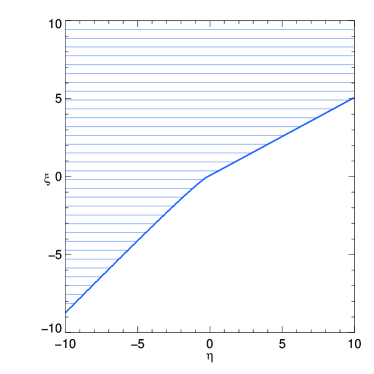
Figure 2: Constraint from the absence of photon decay. The filled region in the parameter space is the one excluded by the observation of gamma rays of energies up to $\sim 50$ TeV.

The joint constraints imposed by both vacuum Čerenkov and photon decay are shown in Fig. 3. We see that these two reactions are already enough for ruling out most of the parameter space. Next we shall see that by taking into account also the process of photon annihilation this constraint can be further improved.

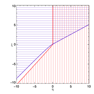
Figure 3: The graph shows the combined observational constraint derived from the absence of vacuum Čerenkov effect and gamma decay. The horizontal blue shading identifies the region excluded by gamma decay, the vertical red one by Čerenkov. Although not visible there is a tiny region of positive $\xi$ and $\eta$ allowed by present observations, and there is a barely visible region of positive $\xi$ and negative $\eta$. Also the diagonal is in the interior of the allowed region.

III.4 Photon annihilation: $\gamma\,\gamma\to e^{+}\,e^{-}$

In standard QED two photons can annihilate to form an electron-positron pair. If one of the photons has energy $\omega_{0}$, the threshold for the reaction occurs in a head-on collision with the second photon having the momentum (equivalently energy) $k_{\rm LI}=m^{2}/\omega_{0}$. For $k_{\rm LI}=10$ TeV (which will be relevant for the observational constraints) the soft photon threshold $\omega_{0}$ is approximately 25 meV, corresponding to a wavelength of 50 microns.

In the presence of Lorentz violating dispersion relations the threshold for this process is in general altered, and the process can even be forbidden. Moreover, as noticed by Kluźniak Kluzniak , in some cases there is an upper threshold beyond which the process does not occur. In this section we discuss how the thresholds depend on the Lorentz violating parameters. We then discuss the observational consequences and constraints that can be obtained using the absorption of TeV gamma rays of extragalactic origin by the intervening infrared (IR) background.

The threshold equation for photon annihilation can be obtained by modifying our previous analysis of photon decay. The difference is that the initial state includes two photons rather than one. We are interested in the case where one of the photons has low energy (IR), hence for that photon the modification in the dispersion relation can be neglected. The threshold theorem (cf. Sect. III.1) tells us that the threshold configuration is a head-on collision. Denoting the IR photon energy by $\omega_{0}$, the total four-momentum of the initial state thus takes the form $k_{\rm 4,in}=(\omega(k)+\omega_{0},k-\omega_{0},0,0)=:(\omega^{\prime},k^{\prime},0,0)$.

To adapt our previous calculation, we need only replace $k$ by $k^{\prime}=k-\omega_{0}$ and $\omega(k)$ by $\omega^{\prime}(k^{\prime})=\omega(k^{\prime}+\omega_{0})+\omega_{0}$. Expanding one gets $\omega(k^{\prime}+\omega_{0})=k^{\prime}+\omega_{0}+(\xi/2)(k^{\prime}+\omega_{0})^{n-1}+\cdots$. Since $\omega_{0}\ll k$, and the last term is already Planck-suppressed (or, if $n=2$, suppressed by the small value of $\xi$), we can neglect $\omega_{0}$ in that term. This yields the approximation $\omega^{\prime}(k^{\prime})=k^{\prime}+(\xi^{\prime}/2)(k^{\prime})^{(n-1)}$, where $\xi^{\prime}$ is defined by

$$\xi^{{}^{\prime}}=\xi+\frac{4\omega_{0}}{(k^{\prime})^{(n-1)}}.$$ (45)

The kinematic equation for photon annihilation is thus obtained from that for photon decay (31) by the replacements $k\rightarrow k^{\prime}$ on the lhs and $\xi\rightarrow\xi^{\prime}$ on the rhs. We can further neglect the difference between $k^{\prime}$ and $k$ on the lhs since $\omega_{0}\ll k$, hence to a sufficiently good approximation we can use the kinematic equation

$$0=F(k,y):=-\frac{m^{2}}{k^{n}}+\left(\xi+\frac{4\omega_{0}}{k^{(n-1)}}\right)y\left(1-y\right)-\eta y\left(1-y\right)\left[y^{(n-1)}+\left(1-y\right)^{(n-1)}\right].$$ (46)

The variable $y$ is defined by $y=p/k$, where $p$ is one of the lepton momenta. Our analysis of the thresholds is based on Eq. (46).

As in the case of photon decay, the thresholds occur at the symmetric value $y=1/2$ only for certain ranges of the parameters $\xi$ and $\eta$. The analysis for photon annihilation is more complicated however since for $n\geq 3$ the dependence of Eq. (46) on $k$ and $y$ does not separate, unlike in Eq.(31). Thus it is not simply a matter of finding the value of $y$ between zero and unity for which $F(k,y)$ is maximum. Analyzing the threshold structure is a rather lengthy and complicated process, so we have placed the details in an Appendix. The analysis reveals a number of unexpected features that thresholds can have in the presence of Lorentz violating dispersion, with intricate dependence on the Lorentz violating parameters. Here we summarize the results in the cases $n=2,3$, and apply them to obtain further observational constraints.

We obtain results valid for any value of the soft photon energy $\omega_{0}$ and “electron” mass $m$ by employing appropriately scaled quantities:

$$\beta=k/k_{\rm LI},\qquad\widetilde{\eta}=\eta(m^{2(n-1)}/\omega_{0}^{n}),\qquad\widetilde{\xi}=\xi(m^{2(n-1)}/\omega_{0}^{n})$$ (47)

where $k_{\rm LI}$ is the standard lower threshold $m^{2}/\omega_{0}$ The basic threshold structure will be given in terms of these variables. For the case of most interest to us, $n$ is 3 and $m$ is the electron mass. For $\omega_{0}=25$ meV we then have $\xi=(\omega_{0}^{3}/m^{4})\,\widetilde{\xi}\simeq 2.3\,\widetilde{\xi}$, and similarly for $\eta$.

It is worth noting that while we have been thinking of $\omega_{0}$ as fixed and determining the corresponding high energy threshold, it can be viewed the other way around. The parameter $\beta$ can also be written as $\omega_{0}/(m^{2}/k)$. If now $k$ is considered fixed then $\omega_{0}$ is the modified soft photon threshold and $m^{2}/k=\omega_{\rm LI}$ is the corresponding Lorentz invariant threshold. Therefore $\beta$ has also the interpretation $\omega_{0}/\omega_{\rm LI}$, that is the factor by which the soft photon threshold is shifted at fixed hard photon energy $k$. This interpretation is valid for lower thresholds only however. There is in fact never an upper threshold for the soft photon at fixed $k$ (as long as $\omega_{0}\ll k$).

III.4.1 Photon annihilation thresholds for n=2

For $n=2$ the threshold configuration is always the symmetric one. The contour of threshold $\beta$ is given by the straight line

$$\widetilde{\xi}=\widetilde{\eta}+4\frac{1-\beta}{\beta^{2}}.$$ (48)

The $\widetilde{\xi}$-intercept decreases monotonically from $\infty$ to $-1$ for $\beta<2$, and increases monotonically from $-1$ to $0$ for $\beta>2$. Hence the process is forbidden below the line $\widetilde{\xi}=\widetilde{\eta}-1$. The parameter $\beta$ gives the lower threshold for $\beta<2$ and the upper threshold for $\beta>2$. If the lower threshold is greater than unity, then the upper threshold exists and is given by $\beta/(\beta-1)$. The maximum lower threshold $\beta=2$ corresponds to $k=2k_{\rm LI}=2m^{2}/\omega_{0}$.

III.4.2 Lower threshold of photon annihilation for $n=3$

For $n=3$ the threshold configuration is not always symmetric in the outgoing momenta. Instead of straight parallel lines for the contours of threshold $\beta$ we find a more complicated structure. Figure 4 shows the regions in the parameter plane where the threshold configuration is symmetric or asymmetric or does not exist at all, and a contour plot of the lower threshold is shown in Figure 5.

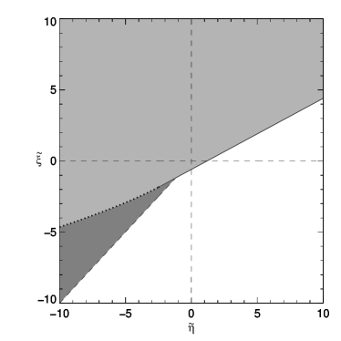
Figure 4: Regions where the lower threshold for photon annihilation with $n=3$ is determined by the symmetric configuration (light grey region), the asymmetric one (dark grey region) or the reaction does not occur (white region). The dotted line is the locus of points where the contour of constant $\beta\leq 1.5$ switches smoothly from the asymmetric to the symmetric solution.

Figure 5: Contours of constant lower threshold $\beta={\rm const}$. For $\beta\leq 1.5$ these correspond to symmetric configurations above the dotted line and asymmetric ones below. For $\beta>1.5$ there are only asymmetric lower thresholds and the contours terminate at the symmetric $\beta=1.5$ contour. The end of the dotted line is at $(\widetilde{\eta},\widetilde{\xi})=(-64/27,\,-48/27)$, and the $\beta=1.5$ contour meets the diagonal at $\widetilde{\eta}=\widetilde{\xi}=-32/27$.

The threshold can be symmetric only for $\beta\leq 1.5$. The symmetric part of the contour is given by the straight line

$$\widetilde{\xi}=\frac{\widetilde{\eta}}{2}+\frac{4(1-\beta)}{\beta^{3}},$$ (49)

restricted to the region above the line $\widetilde{\xi}=-4/\beta^{2}$. Below this line the $\beta$-contour switches to the asymmetric threshold, and is given by

$$\widetilde{\xi}=\widetilde{\eta}-\frac{4}{\beta^{2}}+\sqrt{-\frac{8\widetilde{\eta}}{\beta^{3}}}.$$ (50)

The joining point of the symmetric and asymmetric parts of the $\beta$-contour is at $(\widetilde{\eta}_{\rm join},\widetilde{\xi}_{\rm join})=(-8/\beta^{3},\,-4/\beta^{2})$. As $\beta$ varies from 0 to $1.5$ these joining points trace out the curve $\widetilde{\xi}_{\rm join}=-(-\widetilde{\eta})^{2/3}$. The asymmetric threshold contours for $\beta>1.5$ terminate at the symmetric $\beta=1.5$ contour, and accumulate above the diagonal as $\beta\rightarrow\infty$. The precise degree of asymmetry at threshold, i.e. the ratio of electron momentum to incoming hard photon momentum, is given by $y=(1\pm\sqrt{z_{a}})/2$, where $z_{a}=(\widetilde{\xi}+4/{\beta^{2}})/\widetilde{\eta}$.

III.4.3 Upper threshold of photon annihilation for $n=3$

Upper thresholds exist for $n=3$ only below the diagonal and between the $\beta=1.5$ and $\beta=\infty$ (which gives the same line as $\beta=1$) symmetric contours (49). For a given $\beta$ the threshold is symmetric in the region above the line $\widetilde{\xi}=-4/\beta^{2}$ and asymmetric below, where the contour is given by the curve (50). The regions of symmetric and asymmetric upper thresholds for $n=3$ are shown in Figure 6.

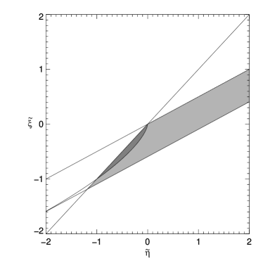
Figure 6: Regions where the upper threshold is determined by the symmetric configuration (light grey region) or the asymmetric one (dark grey region). In the white region below the light grey and below the diagonal the reaction never occurs, and in the rest of the white region there is a lower threshold but no upper threshold.

The boundary of the lens shaped region next to the diagonal is determined by the curve $\widetilde{\xi}_{\rm join}=-(-\widetilde{\eta})^{2/3}$ consisting of the points where the symmetric and asymmetric segments join. The bottom of the lens meets the diagonal at $\widetilde{\eta}=\widetilde{\xi}=-1$ where the symmetric $\beta=2$ line crosses, so asymmetric upper thresholds exist only for $\beta>2$. The lower boundary of the region of upper thresholds is the $\beta=1.5$ line, which meets the diagonal at $\widetilde{\eta}=\widetilde{\xi}=-32/27$.

The possibility of upper thresholds for photon annihilation has been previously discussed by Kluźniak Kluzniak , who gave results for the values $\eta=0$, $\xi=-1$, and $\eta=\xi=-1$ in the $n=3$ case. It seems that only the symmetric configuration was examined in Kluzniak , hence his results cannot fully agree with ours in cases where the asymmetric configuration is important. For the case $\eta=0$, and negative $\xi$, our results show that there is a symmetric upper threshold only for $\widetilde{\xi}$ values above the $\beta=1.5$ line, i.e. for $\widetilde{\xi}>-16/27$. Our upper threshold agrees with that of Kluzniak in the limit $|\widetilde{\xi}/4|=|\xi m^{4}/4\omega_{0}^{3}|\ll 1$. The left hand side is unity for $\xi=-1$ and $\omega_{0}\simeq 20$ meV, hence our results agree approximately provided $\omega_{0}$ is greater than about $\simeq 40$ meV. In the diagonal case, while our results for the symmetric configuration agree in the same limit, we have seen that there is no upper threshold since asymmetric configurations exist for arbitrarily large $\beta$.

III.4.4 Observations and constraints from absence of deviations from standard photon annihilation

The Čerenkov and photon decay constraints leave open an infinite wedge-shaped region including the diagonal in the lower left quadrant for the case $n=3$. A constraint from agreement with standard photon annihilation would be complementary to these and hence has the potential to confine the allowed region to a small neighborhood of the origin. Such a constraint is provided by indirect observations of annihilation of high energy gamma rays from blazars on the cosmic background radiation (CBR). Since there is presently considerable uncertainty regarding both the background radiation and the nature of the sources, the constraint that can be extracted is not yet very precise however.

Another limitation of the present work arises from the fact that each observed gamma ray has the opportunity to interact with soft photons at any energy above the threshold, so to compare with observation one should compute the absorption using the Lorentz violating dispersion relation, integrating over all target frequencies. Such an investigation lies outside the scope of the present paper, so we shall only attempt to roughly characterize how large a threshold shift might be compatible with current observations.

We now summarize the observational situation. The BL Lac objects Mkn 421 and Mkn 501 are a type of blazar emitting high energy gamma rays whose observed spectrum reaches 17 TeV in the case of Mkn 421 Mkn421 and 24 TeV in the case of Mkn 501 Mkn501 . The source power spectra are reconstructed accounting for absorption via photon annihilation on the intervening CBR, which ranges from the near infrared (NIR, $\sim 1~{}\mu$m) to the cosmic microwave background (CMBR, $\sim 1000~{}\mu$m). Currently we have a good knowledge of the NIR and CMBR but uncertainties remain regarding the distribution in the intermediate, mid infrared ($\sim 10~{}\mu$m) and far infrared ($100~{}\mu$m), regions (see e.g. Figure 1 of Aharonian:2001cp or the discussion in stecker01 ). Some models of the IR background imply a source spectrum for Mkn 501 with an unexpected amount of radiation (a “pile-up”) above $10$ TeV Protheroe:2000hp ; Aharonian:2001cp . If such IR backgrounds are correct, the pile-up might be due to a process producing enhanced emission at energies larger than $10$ TeV Aharonian:2001cp , or it might be explained by anomalously low absorption caused by an upward shift of the threshold due to Lorentz violation ACP ; Kifune:1999ex ; Kluzniak ; Protheroe:2000hp ; Aloisio:2000cm . However, recent work SG01 ; stecker01 based on improved reconstructions of the FIRB and on a new analysis of the gamma ray flux from Mkn 501 supports the view that current observations are consistent with the predictions of standard Lorentz invariant theory up to 20 TeV. Even without resolving the question of the pile-up, it seems well established that some degree of photon absorption has been observed up to 20 TeV, which already provides an interesting constraint on Lorentz violation. Moreover, it is our impression that the suggestions of an anomaly above 10 TeV will likely prove illusory as new observations are made available, confirming the results of SG01 ; stecker01  . We can thus obtain observational constraints from the requirement that the Lorentz violation does not too strongly modify standard Lorentz-invariant thresholds for photon annihilation. The strength of the constraints depends of course on the order $n$ of the Lorentz deformation. The general threshold equation (57) shows that an order unity constraint on $\beta$ translates into an order unity constraint on $\widetilde{\eta}$ and $\widetilde{\xi}$, which corresponds to an order $\omega_{0}^{n}/m^{2(n-1)}$ constraint on $\eta$ and $\xi$. Since all studies seem to agree that more or less standard Lorentz-invariant absorption is occurring for gamma rays up to 10 TeV, we shall use the corresponding soft photon threshold of $\omega_{0}=25$ meV $\sim$ 50 $\mu$m as a numerical benchmark. One then has $\omega_{0}^{2}/m^{2}\sim 10^{-15}$ for $n=2$, $\omega_{0}^{3}/m^{4}\sim 1$ for $n=3$, and $\omega_{0}^{4}/m^{6}\sim 10^{15}$ for $n=4$. Hence only the $n=2$ and $n=3$ cases can provide interesting constraints. Note that in the $n=3$ case, which is of most interest to us, the dependence on $\omega_{0}$ is cubic, so for example a constraint at $2\,\omega_{0}$ is eight times weaker than a constraint at $\omega_{0}$, while one at $\omega_{0}/2$ is eight times stronger. This means also that there could be strong deviations in absorption for, say, 20 TeV gamma rays, and yet little deviation for 10 TeV gamma rays, since the standard soft target threshold $m^{2}/E$ is half as large for the 20 TeV gamma rays.

To formulate the constraints we begin by identifying the contour in the $\xi$–$\eta$ plane, for which the threshold is not shifted away from the Lorentz-invariant value. For $n=2$ this no-shift contour is given by the diagonal $\xi=\eta$ (corresponding to equal speeds of light for electrons and photons), which is independent of the soft photon energy $\omega_{0}$. For $n=3$ the contour is given by the joined symmetric and asymmetric $\beta=1$ contours (49) and (50) converted to the unscaled parameters,

$$\xi = \displaystyle{\frac{\eta}{2}}\qquad\qquad\qquad\qquad\qquad\mbox{for $\eta>-8\omega^{3}_{0}/m^{4}$}$$ (51)

$$\xi = \displaystyle{\eta-\frac{4\omega_{0}^{3}}{m^{4}}+\sqrt{-\frac{8\omega_{0}^{3}}{m^{4}}\eta}}\qquad\mbox{otherwise}$$ (52)

The symmetric part is independent of $\omega_{0}$ but the joining point and the asymmetric part are not.

Above the no-shift contour, Lorentz violation lowers the threshold. Since the shift would be larger for higher energy gamma rays this might, depending on the details of the IR background spectrum, enhance the “pile-up” in the reconstructed source spectrum if the IR backgrounds of Protheroe:2000hp are used, or it might produce a pile-up where one did not otherwise exist if the IR background of stecker01 is used. We thus consider it unlikely that there is much downward shift of the threshold. In any case, nearly all of the region above the no-shift line is already excluded by the photon decay and Čerenkov constraints.

Below the no-shift contour, Lorentz violation raises the threshold. We now consider the constraints this can yield in the cases $n=2$ and $n=3$.

$n=2$ Photon annihilation constraints.

Constraints in the $n=2$ case have been previously examined in Ref. SG01 , although it was not realized there that the maximum upper shift is $\beta=2$, beyond which the process does not occur at all. The $\beta=2$ contour (48) is a line of unit slope and $\widetilde{\xi}$–intercept $-1$ in the scaled parameters, hence unit slope and $\xi$–intercept $-\omega_{0}^{2}/m^{2}\sim-10^{-15}$. As long as the 25 meV photons annihilate at least with 20 TeV photons (whose normal threshold is 12.5 meV), the parameters must lie above this line.

$n=3$ Photon annihilation constraints.

For $n=3$ the contours of constant threshold in the scaled parameters $\widetilde{\eta}$ and $\widetilde{\xi}$ are shown in Fig. 5. The process does not occur for parameters below a broken line consisting of the diagonal up to $\widetilde{\eta}=\eta\times m^{4}/\omega_{0}^{3}=-32/27$, and the line of slope $1/2$ for greater $\widetilde{\eta}$. If absorption at $\omega_{0}$ is occurring for any hard gamma ray, the parameters must lie above this broken line, so in particular everything on and below the diagonal is excluded for $\widetilde{\eta}<-32/27$. For $\omega_{0}=25$ meV this corresponds to $\eta<-2.3\cdot 32/27\approx-2.7$. This is important, since it is a strong constraint excluding most of the diagonal, which has been preferred by some researchers ACP ; Aloisio:2000cm . It is likely that a much stronger constraint holds however, restricting the lower threshold at 25 meV to be not more than some number of order unity times its usual value. We have indicated in Fig. 7 the form of the region below the no-shift contour and above the shift-less-than-$\beta$ contour for $\beta$ equal to 10, 5, 2 and 1.5. A stronger constraint would not exclude more of the diagonal, but it has the potential to chop off the infinite wedge of Figure 3 at around the same place it excludes the diagonal.

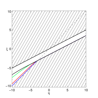
Figure 7: The unfilled region indicates parameters allowed if the lower threshold for a soft photon of 25 meV is $(a)$ not shifted down and $(b)$ not shifted up by more than 1.5, 2, 5, 10, and infinity. The upper line is the no-shift contour. No curvature due to the asymmetric solution is visible for this line because the junction point as defined in Eq. (51) is at $\eta=-20$. The line for the existence of a lower threshold is the lowest line. It is coincident with the symmetric $\beta=1.5$ line below the diagonal and with the (dashed) diagonal below the crossing point. The curves stemming from the $\beta=1.5$ contour are the asymmetric contours for $\beta=10,5,2$, with lower values of $\beta$ corresponding to the curves with less slope.

III.5 QED processes without thresholds

We now consider two QED effects that occur in the presence of Lorentz violation without any threshold, velocity dispersion of photons in vacuo and photon splitting. The former will eventually provide competitive constraints on $\eta$ and $\xi$ respectively, but the latter has too slow a rate to be important.

III.5.1 Velocity dispersion of photons

Gamma-ray bursts (GRB’s) are explosive extragalactic events that release a large number of high energy photons with a flux that varies rapidly in time. It was therefore realized Acea ; Ellis:1999sd that they can provide interesting constraints or possible observations of Planck scale suppressed Lorentz violation in the dispersion relation for photons (a possibility noted long ago in Pav ). The reason is that while propagating over such a long distance even tiny differences in group velocity could produce detectable time differences between the arrival at Earth of photons of different energy.

For photons with Lorentz breaking dispersion relations of order $n$, $\xi$ is related to the fractional variation in group velocity by

$$\xi=\frac{2}{n-1}\frac{M^{n-2}}{k_{1}^{n-2}-k_{2}^{n-2}}\frac{\Delta c}{c}.$$ (53)

An upper limit on the difference in arrival times of photons from the same event provides an upper limit on the relative speed difference, if one assumes there is no conspiracy of different emission times cancelling different propagation times. Together with the energies of the different photons, such observations provide a constraint on $|\xi|$.

The strongest constraint available today comes from GRB 930131 , a gamma ray burst at a distance of 260 Mpc that emitted gamma rays from 50 keV to 80 MeV on a timescale of milliseconds sommer . Schaefer schaefer finds the upper limit $\Delta c/c<9.6\cdot 10^{-19}$ for photons of energy $k_{1}=78.6$ MeV, and $k_{2}=30$ keV. This yields the constraint $|\xi|<122$ for $n=3$. This is weaker than the constraint we have from photon annihilation, hence time of flight data do not at present strengthen our constraints for $n=3$. For $n=4$ dispersion the bound on $|\xi|$ is on the order of $|\xi|<10^{18}$, so we get no interesting constraint for $n>3$. The situation for $n=3$ will be significantly improved in the future thanks to GLAST, the gamma ray large area space telescope, which should be able to set limits of order unity on $\xi$ Norris:1999nh .

III.5.2 Photon Splitting

The photon splitting processes $\gamma\rightarrow 2\gamma$ and $\gamma\rightarrow 3\gamma$, etc. do not occur in standard QED. Although there are corresponding Feynman diagrams (the triangle and box diagrams), their amplitudes vanish. In the presence of Lorentz violation these processes are generally allowed when $\xi>0$. However, the effectiveness of this reaction in providing constraints depends heavily on the decay rate. We now give an estimate of this rate, independent of the particular form of the Lorentz violating theory, which indicates that the rate involves at least four Lorentz violating factors, so is apparently too small to be relevant at observed photon energies.

We carry out the analysis allowing for any terms in the amplitude consistent with gauge and translation invariance. The particular form of Lorentz violation considered in this paper also preserves rotation invariance in a preferred frame, however the following argument will not use that condition. Since gauge invariance is preserved, the amplitude for the process $\gamma\rightarrow N\gamma$ should arise from a term that is a scalar formed from $N$ factors of the electromagnetic field strength $F_{ab}$ corresponding to the external photon legs. For each photon, $F^{({\rm s})}_{ab}\sim k_{[a}\epsilon_{b]}$, where $k_{a}$ is the 4-momentum and $\epsilon_{b}$ is the polarization vector.

In the Lorentz invariant case the equations of motion imply that $k_{a}$ is a null vector and $k_{a}\epsilon^{a}=0$. Energy-momentum conservation then implies that these 4-momenta are all parallel, so being null they are orthogonal to each other and to all the polarization vectors. The rate thus vanishes for two different reasons. First, since the momenta are necessarily all parallel, the phase space has vanishing volume. Second, the rate must be a scalar formed by contracting these four field strengths using only the metric. Any such contraction vanishes since it must involve contractions of the momenta with each other or with the polarizations. Hence the amplitude vanishes. In the case of an odd number of photons, another reason for vansihing of the amplitude is Furry’s theorem, which states that the sum over loops with an odd number of electron propagators vanishes.

If there is Lorentz violation then none of the above reasons for a vanishing rate apply. First of all the $N$-odd amplitudes are no more guaranteed to vanish. Indeed for sufficiently general implementations of Lorentz violation the Furry theorem can be violated (see e.g. the discussion of the Furry theorem and its violation in the extended QED Kostelecky:2001jc ). Secondly, the contractions of the field strengths might involve not just the metric but also a Lorentz violating tensor (for example $u^{a}u^{b}$ in the rotation invariant case, where $u^{a}$ is the unit timelike vector specifying the preferred frame.) Finally, in the presence of Lorentz violation the photon four-momenta are in general not null vectors hence they need not be parallel and they need not vanish upon contraction. (To satisfy energy-momentum conservation $\xi$ must be positive.)

In order for the phase space to not have vanishing volume, at least one of the 4-momenta must involve a Lorentz-violating factor $\delta=\xi(k/M)^{n-2}$. This is not enough for the amplitude to not vanish however. For $\gamma\rightarrow N\gamma$ with $N=3$ or 4 the contraction of the 3 or 4 field strength tensors $F^{({\rm s})}_{ab}\sim k_{[a}\epsilon_{b]}$ using only the metric involves at least two vanishing contractions, and for larger $N$ there are more. One of those vanishing contractions can be rendered nonzero by the single Lorentz violating factor already invoked on an external photon momentum, but the other one requires either another such factor, or a Lorentz violating tensor in the operator whose matrix element is being computed. Such a tensor comes with some coefficient with dimensions determined by the dimension of the operator. We also use the symbol $\delta$ to indicate this sort of Lorentz-violating factor.

The possible contributions to the amplitude will therefore be suppressed by at least two factors of $\delta$. The rate goes like the square of the amplitude, hence we infer that at energies well above the electron mass the decay rate must behave as $E\delta^{4}$ or slower, where $E$ is the initial photon energy. (There is an additional factor of $\alpha^{N}$ if we consider standard QED diagrams for which each external photon leg comes with a factor of the electric charge in the amplitude.)

The lifetime is therefore at least of order $\delta^{-4}E^{-1}$, which for a photon of energy 50 TeV is $10^{-29}\delta^{-4}$ seconds. Such 50 TeV photons arrive from the Crab nebula, about $10^{13}$ seconds away, so the best constraint (i.e. if there is is no further small parameter such as $\alpha^{N}$ or $1/16\pi^{2}$ in the decay rate) we could possibly get on $\delta$ from photon splitting is $\delta\lesssim 10^{-10}$. For $n=2$ this is not competitive with the other constraints already obtained. For higher $n$, each contribution arising from an operator of dimension greater than four will be suppressed by at least one inverse power of the scale $M$. For example, the contributions from $n=3$ deformations to the dispersion relation will yield $\delta\sim\xi E/M$. In this case the strongest conceivable constraint on $\xi$ would be of order $\xi\lesssim 10^{4}$, and even this is not competitive with the other constraints we have found.

III.6 Combined Constraints

Having completed our discussion of photon–electron processes we now turn to the determination of the global constraints that can be derived from the combination of all the above results. The photon splitting and the time of flight constraints are not as strict as those determined by the other considered interactions, at least for quadratic and cubic deformations, although in the future time of flight constraints may become competitive.

III.6.1 n=2

In the case of quadratic deviations only the difference $\xi-\eta$ is constrained. The vacuum Čerenkov effect yields $\xi-\eta>-10^{-17}$, while photon decay provides the constraint $\xi-\eta<10^{-16}$. Together these confine $\xi-\eta$ to a small neighborhood of zero. The photon annihilation “likelihood region” would just impose $\xi-\eta\lesssim 10^{-15}$, which does not further strengthen the constraint.

III.6.2 n=3

Putting together the constraints from the three photon–electron interactions previously considered we obtain a remarkably small allowed region in the $\eta$–$\xi$ plane (see Figure 8).

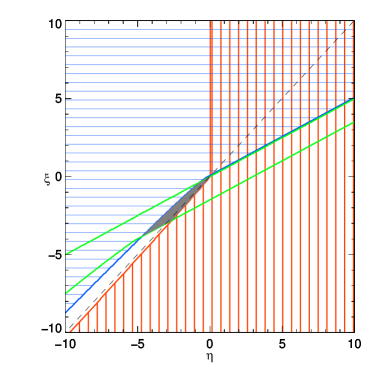
Figure 8: Combined constraints on the photon and electron parameters, for the case $n=3$. The regions excluded by the photon decay and Ĉerenkov constraints are lined horizontally in blue and vertically in red respectively. The region between the two diagonal green lines is where the threshold for the annihilation of a gamma ray with a 25 meV photon ranges from its standard value (upper diagonal green line) to not more than twice that value. The shaded patch is the part of the allowed region that falls between these gamma annihilation thresholds. The dashed line is $\xi=\eta$. 

The photon decay and Čerenkov constraints exclude the horizontally and vertically filled regions respectively. The allowed region lies in the lower left quadrant, except for an exceedingly small sliver near the origin with $0<\eta\;\raisebox{-3.44444pt}{$\stackrel{{\scriptstyle\textstyle<}}{{\sim}}$}\;10^{-3}$ and a small triangular region ($-0.16\;\raisebox{-3.44444pt}{$\stackrel{{\scriptstyle\textstyle<}}{{\sim}}$}\;\eta<0$, $0<\xi\;\raisebox{-3.44444pt}{$\stackrel{{\scriptstyle\textstyle<}}{{\sim}}$}\;0.08$) in the upper left quadrant. The discussion of the photon annihilation threshold in subsection III.4.4 indicates that, although no firm constraint can be given at present, the allowed region cannot lie too far from the corridor between the two roughly parallel diagonal lines. These lines indicate where the threshold for the annihilation of a gamma ray with a 25 meV photon ranges from its standard value (upper diagonal green line) to not more than twice that value.

If future observations of the blazar fluxes and the IR background yield agreement with standard Lorentz invariant kinematics, the region allowed by the photon annihilation constraint will be squeezed toward the upper line ($k_{\rm th}\approx k_{\rm s}$).

Time of flight constraints for high energy photons currently constrain $\xi$ to be less than $\sim 100$ at best, but future observations should allow such constraints to further narrow the allowed region towards the origin.

III.6.3 n=4

The case of quartic deviations is unfortunately just mildly constrained from the available observations. The order of magnitude allowed for the parameters is as small as $10^{11}$ (from Čerenkov) for the electron–photon vertex interactions.

IV Interactions with protons, neutrinos, and muons

We have focused so far on effects involving just electrons and photons, in order to determine the strongest available combined constraints. We now briefly discuss some other interactions that are realizable with a violation of Lorentz invariance, and which can now or in the future provide further constraints or observations of Lorentz violation.

IV.1 Alternative vacuum Čerenkov effects: protons, neutrinos and muons

The former discussion of the vacuum Čerenkov effect can be applied also for any other particle that couples to photons, using the same kinematic equations. Since the strength of the observational constraint is determined by the smallness of the ratio $m^{2}/p^{n}_{\rm max}$, smaller masses or larger energies generally lead to stronger constraints. However, in the case of neutral particles that couple to photons only through higher multipole moments the rate must also be considered. We summarize in Table 2 the values of the quantity $m^{2}/p_{max}^{n}$.

Table 2: Typical values for different particles for the actual or potential constraints from absence of the vacuum Čerenkov effect.

	$\nu$		$e^{-}$		$\mu^{-}$		$p^{+}$
$m$	$\lesssim 1$ eV		$0.511$ MeV		$105$ MeV		$938$ MeV
$p_{\rm max}$	$\sim 1$ TeV – $10^{20}$ eV		$\sim 100$ TeV		$\sim 1$ PeV		$\sim 5\cdot 10^{19}$ eV
	$\>n=2\>$	$\>\>\sim 10^{-24}$ – $10^{-40}\>\>$	$\>n=2\>$	$\>\>\sim 3\cdot 10^{-17}\>\>$	$\>n=2\>$	$\>\>\sim 10^{-14}\>\>$	$\>n=2\>$	$\>\>\sim 4\cdot 10^{-22}\>\>$
${m^{2}}/{p_{\rm max}^{n}}$	$\>n=3\>$	$\>\>\sim 10^{-8}\>\,$ – $10^{-32}\>\>$	$\>n=3\>$	$\>\>\sim 3\cdot 10^{-3}\>\>$	$\>n=3\>$	$\>\>\sim 10^{-1}\>\>$	$\>n=3\>$	$\>\>\sim 8\cdot 10^{-14}\>\>$
	$\>n=4\>$	$\>\>\sim 10^{8}\;\,\,$ – $10^{-24}\>\>$	$\>n=4\>$	$\>\>\sim 3\cdot 10^{11}\>\>$	$\>n=4\>$	$\>\>\sim 10^{12}\>\>$	$\>n=4\>$	$\>\>\sim 2\cdot 10^{-5}\>\>$

IV.1.1 Protons

Very strong constraints can be obtained using the ultra high energy protons in cosmic rays, up to the GZK cutoff of $5\cdot 10^{19}$ eV. The identity of these particles has been called into question by the candidate events beyond the GZK cutoff as described in Sect. IV.2. However, even if the highest energy events do not originate with protons, there is strong evidence that protons up to the GZK cutoff do exist in cosmic rays Bahcall:2002wi .

The rate of vacuum Čerenkov radiation from charged particles is irrelevant for the determination of constraints since it is very high. (See Sect. III.2.2.) For the parameter region where the threshold occurs with emission of a zero energy photon, the proton can presumably be treated as a point charge so the threshold relations previously obtained for electrons are directly applicable using the proton mass in place of the electron mass, and the parameter $\eta_{p}$ from the proton dispersion relation in place of $\eta_{e}$. This region of parameter space is described in section III.2.

For parameters where a hard photon is emitted at threshold, the role of the partonic structure of the proton needs to be examined, which we have not done. It may turn out that the threshold can be determined by the quark dispersion relation rather than that of the proton. If so, it would be the quark deformation parameter $\eta_{q}$ rather than $\eta_{p}$ that is constrained by observations of non-decaying high energy protons, and one would need to use the quark mass and energy in the threshold relations. In this case the proton may be destroyed rather than just slowed by vacuum Čerenkov radiation, however that distinction is irrelevant for the determination of constraints, since either way high energy protons would not travel long distances.

In estimating constraints we ignore here the possible role of partonic structure, and simply use the proton mass and energy in the threshold formulae derived in section III.2 for point particles, with the understanding that for hard emission thresholds the constrained parameter may be $\eta_{q}$ rather than $\eta_{p}$, and the numbers may be off by a few orders of magnitude since the quark mass and energy were not used.

Using the GZK cutoff ($5\cdot 10^{19}$ eV) for the highest energy protons we obtain the following constraints relating the parameter $\xi$ in the photon dispersion relation and $\eta_{p}$ in the proton dispersion relation. For a quadratic deformation of the dispersion relation ($n=2$) the bound is $\eta_{p}-\xi<4\cdot 10^{-22}$. For cubic deformations ($n=3$) the constraints on parameter space have the same form as represented in Figure 1. In the case of the proton the quantity $m^{2}_{p}/p_{\rm max}^{3}$, is of order $10^{-14}$ compared with $10^{-3}$ in the case of $100$ TeV electrons, which means that the boundaries of the allowed region are closer to the $\xi$ axis in the upper half plane and to the diagonal in the lower half plane. However, the qualitative nature of the allowed region is identical. A good constraint is even obtained for the case of quartic ($n=4$) deviations. As shown in section III.2.1, it is the quantity $m^{2}_{p}/(p_{\rm max}^{4})$ that determines the strength of the constraint in this case. For $5\cdot 10^{19}$ eV protons this is approximately $10^{-5}$, still much less than unity and a much better figure than the $10^{11}$ obtained for the $100$ TeV electron. For $n=5$ deviations the strength of the constraint is determined by $m^{2}_{p}/(p_{\rm max}^{5})\sim 10^{3}$, hence one does not obtain even order unity constraints on the coefficients.

IV.1.2 Neutrinos

In the standard model the vacuum Čerenkov reaction with neutrinos, $\nu\rightarrow\nu+\gamma$, is not allowed due to energy-momentum conservation - whether or not the neutrinos are massive. If they are massive energy-momentum conservation cannot be satisfied at all. If they are massless it can only be satisfied if all three particles are strictly parallel, yielding no phase space for the reaction. (Since there is good evidence that neutrinos have mass, we will assume this for the rest of the discussion.) Energy-momentum conservation is the only obstruction for this reaction, since although the neutrino is neutral there is a nonzero matrix element for the process. In particular there are two channels: the charge radius interaction and, if massive, a magnetic moment interaction (see e.g. Rabi ). We therefore see that, as for charged leptons, Lorentz violating dispersion relations can allow the reaction to happen.

In order for the neutrino Čerenkov reaction to give strong constraints on Lorentz violation two conditions must be satisfied: (1) the energies where Lorentz violating terms are comparable to the neutrino mass term in the dispersion relation must be accessible to observation, and (2) the rate of the reaction must be high enough so that it would significantly affect the propagation of observed neutrinos. The first condition is already met since the relevant energy where Lorentz violation becomes important is $100$ MeV (see Table 1), while Super Kamiokande has detected neutrinos over $100$ GeV SuperK and the AMANDA detector has seen neutrinos up to a few TeV Ahrens:2002gq . The second condition is more problematic since both the charge radius and magnetic moment channels are very strongly suppressed.

The best case for current observations would be using AMANDA, since the neutrinos have the highest energy and travel the diameter of the earth after being produced in the atmosphere above the North Pole. We have not carried out a detailed analysis, but an estimate given below suggests that the Čerenkov rate is not high enough to produce interesting constraints with these neutrinos. The energy loss rate depends strongly on the energy however, so atmospheric PeV neutrinos, which are likely to be detected by AMANDA or IceCube (seee.g. AMANDA ), may provide constraints. (The same experiments should detect PeV muons as secondary products of the neutrinos, which would also provide an interesting constraint as seen in Table 2.) Still higher energy neutrinos, up to perhaps $10^{20}$ eV, are expected either as cosmic ray primaries or as a byproduct of cosmic rays G ; Stecker79 . Such high energy neutrinos could be detected by AMANDA Hundertmark , and they could be observed via horizontal or possibly upward air showers using existing detectors like HiRes or future ones such as the Telescope Array Kusenko:2001gj ; Feng:2001ue .

In Table 2 we summarize the typical constraints one can expect from neutrinos in the above mentioned range of energies provided the rate is high enough. Remarkably, the combination of high energies and low mass could give for cosmological neutrinos ($E_{\nu}\gg 1$ PeV) stringent constraints ($\eta_{\nu}\ll 1$) for deviations up to $n=6$.

A calculation of the neutrino vacuum Čerenkov rate is beyond the scope of this article but we provide here a rough estimate that may provide some guidance in this problem. We saw before (Section III.2) there are two types of Cerenkov thresholds depending on the values of $\xi$ and $\eta_{\nu}$: the “soft” one which occurs with emission of a zero energy photon, and the “hard” one in which a photon with energy comparable to the incoming particle is emitted. The decay rate will be much greater in the hard threshold case, so we consider that here. (The soft threshold case may still be relevant well above threshold.)

To show that the rate might be fast enough to provide a useful constraint it suffices to examine the charge radius interaction. This occurs via the emission of a virtual W-boson, hence the amplitude goes like $\kappa k_{4}^{2}/M_{W}^{2}$, where $\kappa$ is a small numerical factor ($\sim\!10^{-6}$) coming from coupling constants and integration measure, $k_{4}^{2}$ is the square of the photon four-momentum, and $M_{W}$ is the W-boson mass. We thus estimate the rate for Čerenkov emission from a neutrino of very high energy $E$ to be $\Gamma\sim(\kappa k_{4}^{2}/M_{W}^{2})^{2}E_{\nu}$. (The factor of $E_{\nu}$ is determined by the phase space integration, which does not involve any Lorentz violating factors well above threshold.) With Lorentz violating dispersion of order $n$ we have $k_{4}^{2}=\xi k^{n}$, hence the rate goes like $\Gamma\sim(\kappa\xi k^{n}/M_{W}^{2})^{2}E_{\nu}$.  Taking the photon energy to be of the same order as the neutrino energy $k\sim E_{\nu}$, this gives a lifetime for emission $\tau\sim\xi^{-2}(E_{\nu}/{\rm PeV})^{-(2n+1)}\times 10^{26n-86}$ seconds. If correct this would be short enough to yield interesting constraints for $n=3$ using atmospheric PeV neutrinos travelling through the earth, since their transit time is of order $10^{-2}$ s.

As a final remark, we note that the related process of photon decay to two neutrinos could also take place in the presence of Lorentz violation. This would yield strong constraints on $\xi$ and $\eta_{\nu}$ provided the rate is high enough. The above estimate suggests that for multi-TeV photons from cosmological sources the rate would indeed be high enough for $n=2,3$.

IV.2 The GZK cutoff

The presence of the GZK cutoff on the ultra high energy (UHE) proton spectrum is due to pion photoproduction: $\gamma\,p\to p\,\pi^{0}$, as previously discussed in the Introduction. The observation of this cutoff also gives constraints on the Lorentz violating coefficients. Current data from the HiRes, Fly’s Eye and Yakutsk experiments strongly indicate that the GZK cutoff is present at a cosmic ray energy of $5\cdot 10^{19}$ eV Bahcall:2002wi . While AGASA reports a number of extra events beyond the expected flux of high energy cosmic rays above $10^{20}$ eV, below $10^{20}$ eV AGASA also shows evidence for the GZK cutoff (see e.g. Figure 1 of Bahcall:2002wi ). Unfortunately, the experimental data are strongly affected by the uncertain energy calibration of each experiment. A systematic analysis of the data allowing for various calibrations is outside the scope of this work, so for now we assume that the published energy calibrations are correct.

We constrain $\eta_{p},\eta_{\pi}$ by determining where the induced modification of the cutoff would disagree with the data. (The incoming photon has low energy and so no useful constraints on $\xi$ are obtained.) The $\eta_{p},\eta_{\pi}$ constraints are quite strong (on the order of $10^{-10}$ for $n=3$) due to the high energy of the reaction.

In the standard Lorentz invariant theory the threshold energy for pion production is $E_{\rm th}=m_{\pi}(2\,m_{p}+m_{\pi})/4\omega_{0}$, so a photon with energy $\omega_{0}\sim 1.3$ meV is at threshold with the proton at the GZK energy. In order to give a constraint on Lorentz violations we consider raising or lowering the UHE proton at threshold with the same $\omega_{0}$. This is equivalent to changing the GZK cut-off as we are modifying the UHE proton energy that interacts with the relevant CMBR photons responsible for the Lorentz invariant GZK effect.

Examination of the data plot in Fig. 2 of Ref. Bahcall:2002wi reveals that if the cutoff were shifted via a Lorentz violating effect down to $2\cdot 10^{19}$ eV or up to $7\cdot 10^{19}$ eV then the theoretical predictions would no longer agree with the data at above a $2\sigma$ confidence level. This energy range therefore provides constraints on $\eta_{p},\eta_{\pi}$. From the threshold theorems of JLMth we again know that in the threshold configuration where the GZK reaction begins to occur the incoming proton and photon collide head on and the outgoing proton and pion 3-momenta are parallel. Energy-momentum conservation in this configuration and the dispersion relations give an equation similar to equation (46) for photon annihilation,

$$0=F(p,x):=-\frac{m^{2}_{p}}{p^{n}}(1-x)^{2}-\frac{m_{\pi}^{2}}{p^{n}}x+\left(\eta_{p}+\frac{4\omega_{0}}{p^{(n-1)}}\right)x\left(1-x\right)-\eta_{p}x\left(1-x\right)\left[x^{(n-1)}+\frac{\eta_{\pi}}{\eta_{p}}\left(1-x\right)^{(n-1)}\right],$$ (54)

where $x=q/p$, and $p$ and $q$ are the initial and final proton 3-momenta.

For $n=2$ the threshold analysis has already been done by Coleman and Glashow CG leading to a constraint $\eta_{\pi}-\eta_{p}<5\times 10^{-24}\,[\omega/\bar{\omega}]^{2}$ for a target photon $\omega$, where $\bar{\omega}=kT_{\rm CMB}=0.235$ meV.

For $n=3$, the presence of the pion in this equation complicates the analysis as there is an additional mass term and the final particles are not interchangeable. The case of equal coefficients ($\eta_{p}=\eta_{\pi}$) has been studied analytically in  Mestres ; Bertolami ; ACP ; Kifune:1999ex ; Aloisio:2000cm and numerically in Major . Here we numerically find the thresholds for the GZK reaction allowing for unequal coefficients in the case $n=3$. The region in the $\eta_{p},\eta_{\pi}$ plane where the thresholds are in the allowed range discussed above are shown in Figure 9, in which the axes are in multiples of $10^{-10}$.

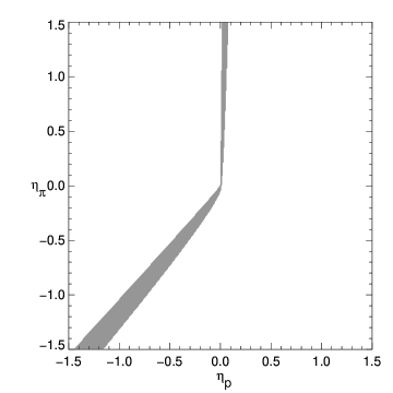
Figure 9: The range of $\eta_{p},\eta_{\pi}$ for $n=3$ dispersion modifications where the GZK cutoff is between $2\cdot 10^{19}$ eV and $7\cdot 10^{19}$ eV. $\eta_{p}$ and $\eta_{\pi}$ are in multiples of $10^{-10}$.

We turn now to the question of the extra AGASA events above $10^{20}$ eV. The AGASA data is sparse in this energy range, and there is not a large, precise data set from other experiments with which AGASA disagrees. The uncertainties in all experiments are large enough that a modified theoretical theoretical spectrum could possibly agree with all experiments at the $1\sigma$ level. One cannot therefore simply disregard the possibility that the flux above $10^{20}$ eV is in fact higher than the standard theoretical prediction.

Previous authors have suggested that the AGASA events above the GZK cutoff could be explained by an upward shift of the GZK cutoff induced by Lorentz violation Mestres ; CG ; Bertolami ; ACP ; Kifune:1999ex ; Major , however this seems incompatible with current data since the cutoff is seen. Another, more subtle possibility is that these events are related to the existence of an upper threshold. We have checked numerically that no upper threshold exists below $10^{20}$ eV within the allowed region of Fig. 9. Nevertheless, the phase space for a reaction begins to close up before the upper threshold is reached. The reduction in phase space would in turn reduce the rate of the GZK reaction leading to a higher than expected count of events at high energies. If the lower threshold were dramatically modified whenever there is an upper threshold then this scenario could not explain the data. However, this is not the case - there are choices of $\eta_{p},\eta_{\pi}$ such that an upper threshold exists and the lower threshold is only slightly modified. Since the lower threshold modifications can be small, the experimental signature of the GZK cutoff could remain unchanged near $5\cdot 10^{19}$ eV while the intensity of the spectrum at high energies increased from its Lorentz invariant prediction. This scenario could perhaps explain the AGASA data and be compatible with other experiments if the upper threshold is low enough that there is a significant phase space reduction just above $10^{20}$ eV. The range of $\eta_{p},\eta_{\pi}$ for which this effect could occur is given in Figure 10.

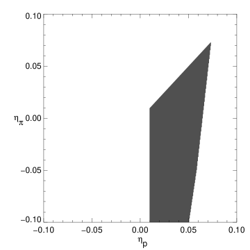
Figure 10: The range of $\eta_{p},\eta_{\pi}$ for $n=3$ dispersion modifications where the GZK cutoff is between $2\cdot 10^{19}$ eV and $7\cdot 10^{19}$ eV and the upper threshold exists below $10^{21}$ eV. $\eta_{p},\eta_{\pi}$ are in multiples of $10^{-10}$. Note that this region does not include the origin, as there is no upper threshold in the Lorentz invariant case.

There we consider the range of parameters for which the lower threshold still lies between $2\cdot 10^{19}$ eV and $7\cdot 10^{19}$ eV but an upper threshold exists below $10^{21}$ eV (so that the induced reduction in phase space could affect the AGASA data).

We have not considered the constraints that can be obtained from the GZK cutoff in the case $n=4$ but it is clear that they are interesting in this case as well, since $1/p_{\rm max}=M/p_{\rm max}=2\cdot 10^{8}$. The $n=3$ constraints are of order $10^{-10}$, hence the $n=4$ ones are of order $10^{-2}$.

IV.3 Neutron stability–Proton instability

If there are different dispersion relations for protons, neutrons, positrons, and neutrinos then protons may be unstable and decay to neutrons at sufficiently high energies. For $n=2$, Coleman and Glashow CG have shown this explicitly. If $n>2$ then the analysis becomes more complicated, but there exist parameters for which the neutron is stable and the proton decays. For example, consider a neutron with $\eta_{n}=-1$ and $n=3$ dispersion relation, and an unmodified proton, electron, and neutrino. At momenta $p_{n}>m_{n}^{2/3}$ the neutron energy-momentum vector becomes spacelike. Since the energy momentum vectors of the other particles are still timelike it is impossible to satisfy energy momentum conservation hence neutron decay does not occur above this energy. This opens the possibility that ultra high energy cosmic rays are neutrons rather than protons, in which case the GZK cutoff for these cosmic rays is irrelevant since neutrons do not interact strongly with CMBR photons. The presence of the observed cutoff can thus be used to constrain the parameters further, and one could also contemplate the possibility that the AGASA events above the GZK cutoff are present because the neutron becomes stable just above the cutoff.

V Combined constraints for a universal Lorentz breaking dispersion relation

Although we have considered so far the case of different Lorentz violating parameters $\eta_{a}$ for different particles, it may be that the underlying quantum gravity physics selects a universal deformation parameter $\eta$. This indeed was the ansatz considered in most of the previous literature. We therefore consider now this special case with $n=3$ deformations.

We start by considering the photon–electron interactions. From Figure 1 and equation (23) we see that the Čerenkov effect limits the available values on the diagonal to a semi-infinite line with $\eta<m^{2}/2p^{3}_{\rm max}$. This corresponds numerically to $\eta\lesssim 10^{-14}$ if we consider the constraint provided by the observation of ultra-high energy protons in cosmic rays. The analysis of photon decay shows that the permitted values on the diagonal $\xi=\eta$ are restricted to the semi-infinite line $\eta<8m^{2}/k_{\rm max}^{3}\sim 8\cdot 10^{-2}$ (using the observation of 50 TeV gamma rays from the Crab nebula). The observation of photon annihilation provides, as previously discussed, a more uncertain constraint. Nevertheless for our purposes it is enough to take into account that some absorption is detected for gamma rays at least up to 10 TeV. We can then take as a definite constraint the line for the existence of a lower threshold as shown in Figure 5. This line meets the diagonal at $\widetilde{\eta}=-32/27$. The problem is now to decide for which $\omega_{0}$ we are sufficiently confident the photon annihilation still takes place. As a reference value we take here again the $\omega_{0}=25$ meV photon previously considered. In this case the region of existence of a lower threshold for the photon annihilation limits the value of $\eta$ to the semi-infinite range $\eta>-2.3\times(32/27)\approx-2.7$.

If the GZK cutoff is confirmed that would establish with certainty that at least some of the UHE cosmic rays are indeed protons. Moreover it would also provide a correspondingly strong constraint on negative values of $\eta$. If the GZK cutoff is within order unity of it’s Lorentz invariant value, $\eta$ is constrained to be $|\eta|\lesssim 10^{-14}$. (Note that this constraint on $\eta$ is so strong as to exclude the region of upper threshold for the GZK process shown in Figure 10.) The upper bound might be further pushed toward zero if one takes into account the Čerenkov effect of high energy neutrinos (see Table 2).

VI Discussion

In this paper we have performed a systematic analysis of the effects of Lorentz violating dispersion on particle reactions, allowing for unequal deformation parameters for different particles. We have analyzed the threshold kinematics and combined the observational constraints where possible. Even when suppressed by the inverse Planck mass, such Lorentz violation can lead to radically new behavior in the kinematics of particle interactions at much lower energies. Reactions previously forbidden can be allowed, lower thresholds can be shifted and upper thresholds can be introduced. The presence of upper thresholds is a feature of Lorentz breaking physics that is not present in Lorentz invariant physics and which can be relevant for observational constraints. Furthermore, we have found that for interactions with identical final particles, the final momenta can be distributed asymmetrically at threshold. While this is a straightforward consequence of the kinematics, it has been previously overlooked in the literature, probably because it is alien to Lorentz invariant physics.

Using these kinematical results, we have seen that a conservative interpretation of observations puts strong constraints on the coefficients $\eta$ and $\xi$ of order $E/M_{\rm P}$ modifications to the electron and photon dispersion relations. The allowed region includes $\xi=\eta=-1$, which has been a focus of previous work ACP ; Kifune:1999ex ; Kluzniak . The negative quadrant has most of the allowed parameter range. Note that in this quadrant all group velocities are less than the low energy speed of light. For modifications of order $(E/M_{\rm P})^{2}$ there are no significant constraints in the electron-photon sector derivable from current observations, due to the fact that the energies of observed particles are too low. However reactions such as proton Čerenkov (in vacuo) or pion production by cosmic rays, for which we have data at much higher energies, can provide good constraints for $(E/M_{\rm P})^{2}$ modifications (although for different particle deformation parameters). Ultra high energy cosmological neutrinos may also provide good Čerenkov constraints at this or even higher orders, since the neutrino mass is much smaller than that of any other particle. The interaction amplitudes are very suppressed however, so it is necessary to accurately calculate the rate and compare it with the travel time of the neutrino.

There are a number of ways to improve the constraints on $O(E/M_{\rm P})$ modifications from electron-photon interactions. Higher energy electrons would not help much since the Čerenkov constraint is already strong, while finding higher energy undecayed photons would squeeze the allowed region onto the line $\xi=\eta$ of Figure 8. To further shrink the allowed segment of this line would require improved knowledge of the infrared background and a reconstruction of the source spectrum from the observed gamma rays in the presence of Lorentz violation. Also, the constraint from time of flight measurement may become competitive using improved detectors.

Other constraints may be provided by additional interactions not considered here. For example, a possible upper threshold for $e^{+}\,e^{-}\rightarrow 2\gamma$ cannot provide a competitive constraint in astrophysical observations since there are other processes by which observed high energy photons can be produced. However, if future electron accelerators can reach energies above $10$ Tev then one can expect to get a good constraint from this reaction. In addition there may be other reactions for which upper thresholds can produce useful constraints at or near currently observed energies. Reactions involving more than two types of particles, such as $\nu\rightarrow e^{-}\,W^{+}$, could also give constraints. It may be possible that by considering a number of such reactions a multi-dimensional parameter space can be usefully constrained.

The idea motivating our work is that Lorentz violation may be a consequence of quantum gravity, in which case the natural scale for the Lorentz violation is the Planck scale. If, as in braneworld scenarios, the quantum gravity scale were to be around a TeV, then the natural scale for Lorentz violation induced by quantum gravity would be the TeV scale. Clearly, the only way such Lorentz violation could be compatible with observations is if it were extremely suppressed compared with this natural scale. This suggests that either TeV scale quantum gravity is wrong, or it does not violate 4d-Lorentz invariance.

In conclusion, the absence of anomalous observations provides stringent constraints on the possibility of Lorentz violation originating at the Planck scale. This in turn gives important information as to the viability of quantum gravity theories that predict 4-d Lorentz violation. We can expect that, as better data at higher energies becomes available, even stronger constraints will be imposed or, alternatively, positive signatures of Lorentz violation may be found. Either way, it is clear that a useful tool for the phenomenological investigation of quantum gravity is now at hand.

Appendix A Photon annihilation thresholds

In this appendix we work out the lower and upper thresholds for the process $\gamma\,\gamma\rightarrow e^{+}\,e^{-}$ as a function of the Lorentz-violating parameters $\eta$ and $\xi$. Our starting point is the kinematic equation (46) derived in section III.4:

$$0=F(k,y):=-\frac{m^{2}}{k^{n}}+\left(\xi+\frac{4\omega_{0}}{k^{(n-1)}}\right)y\left(1-y\right)-\eta y\left(1-y\right)\left[y^{(n-1)}+\left(1-y\right)^{(n-1)}\right].$$ (55)

Here $m$ is the electron mass, $k$ is the magnitude of the incoming hard photon momentum, $\omega_{0}$ is the soft photon energy, $y=p/k$, where $p$ is the magnitude of the electron (or positron) momentum, and the threshold configuration of antiparallel incoming photons and parallel outgoing electron-positron pair has been imposed. This equation follows from (i) energy-momentum conservation, (ii) the dispersion relations for the particles, and (iii) the threshold configuration. To find the lower and upper threshold for given values of $\eta$ and $\xi$ we must determine the minimal or maximal $k$ for which the reaction can occur. According to the threshold theorem (cf. Sect. III.1) these $k$ values always occur with what we just called the threshold configuration, hence we must determine the minimal or maximal $k$ for which there is a solution $(k,y)$ to the kinematic equation (55) with $y$ in the range $[0,1]$. In the Lorentz invariant case the threshold always occurs with the symmetric configuration $y=1/2$, however in the Lorentz-violating case this is not always true.

In order to derive results applicable to any value of the soft photon energy $\omega_{0}$ and “electron” mass $m$, we introduce scaled variables

$$\beta=k/k_{\rm LI},\qquad\widetilde{\eta}=\eta(m^{2(n-1)}/\omega_{0}^{n}),\qquad\widetilde{\xi}=\xi(m^{2(n-1)}/\omega_{0}^{n})$$ (56)

where $k_{\rm LI}$ is the standard lower threshold $m^{2}/\omega_{0}$. In terms of these scaled variables the equation $m^{-2}k^{n}F(k,y)=0$ takes the form

$$G(\beta,y)=\alpha_{n}(y)\,\beta^{n}+\gamma(y)\,\beta-1=0,$$ (57)

where

$$\alpha_{n}(y)=y(1-y)\left(\widetilde{\xi}-\widetilde{\eta}\;\left[y^{n-1}+(1-y)^{n-1}\right]\right)$$ (58)

and

$$\gamma(y)=4\;y(1-y).$$ (59)

Equation (57) is a generalization of those derived by Aloisio et al. Aloisio:2000cm for the specific cases of $n=3,4$ with purely symmetric configurations ($y=1/2$) and equal deformation coefficients ($\widetilde{\xi}=\widetilde{\eta}$).

Figure 11 shows the general behavior of $G(\beta,y)$ (57) for any fixed $y$ (and therefore fixed $\gamma(y)$) and different values of $\alpha$.

Figure 11: Behavior of $G(\beta,y)$ (57) for fixed $y$ and different values of alpha.

From the plot we see that for any $y$ there are either one, two, or zero solutions to the kinematic equation for $\beta$. If there are two solutions, of course only the lower one is a candidate for the lower threshold. The upper one can correspond to an upper threshold, that is, to the highest available value of $\beta$ for which the reaction is kinematically allowed. To our knowledge, the possibility of upper thresholds has been overlooked in all of the previous literature except for Kluźniak Kluzniak (see discussion at end of section III.4.3).

For each $y$ there is a maximal value of the lower root $\beta$ which occurs when $\alpha_{n}$ is such that the curve described by Eq. (57) is tangent to the $\beta$ axis. This occurs for

$$\alpha^{\rm tang}_{n}=-\gamma^{n}\frac{(n-1)^{(n-1)}}{n^{n}},$$ (60)

and, at this tangency point,

$$\beta_{\rm tang}=\gamma^{-1}\frac{n}{n-1}.$$ (61)

If $\beta$ is to be a lower threshold it must lie below this tangency point.

Given values for $\widetilde{\eta}$ and $\widetilde{\xi}$, Eq. 57 implicitly defines zero, one, or two (real positive) solutions for $\beta$ as a function of $y$. A lower threshold corresponds to the global minimum of $\beta$. Our strategy is to first find the local minima and, if there is more than one, determine which is the global minimum.

A local minimum of $\beta(y)$ is characterized by $\beta_{y}=0$ and $\beta_{yy}>0$, where the subscript $y$ denotes derivative with respect to $y$. To find the corresponding conditions on $G$ we use the fact that $G(\beta(y),y)$ is identically zero, hence its total derivative with respect to $y$ vanishes: $G_{\beta}\beta_{y}+G_{y}=0$, where the subscripts on $G$ denote partial derivatives. The second total derivative of $G(\beta(y),y)$ with respect to $y$ also vanishes. At a stationary point where $\beta_{y}=0$, this yields $G_{\beta}\beta_{yy}+G_{yy}=0$. Thus the conditions for $\beta(y)$ to be local minimum are

$$\beta_{y}=-G_{y}/G_{\beta}=0\qquad\qquad{\rm and}\qquad\qquad\beta_{yy}=-G_{yy}/G_{\beta}>0.$$ (62)

It is clear from Fig. 11 that $G_{\beta}$ is always positive at the lower root of $G=0$, and vanishes only at the tangency value of $\alpha$. Since only the lower root can be a lower threshold, we have two necessary conditions to be a lower threshold:

$$G_{\beta}>0\qquad\qquad{\rm and}\qquad\qquad G_{yy}<0.$$ (63)

We now use these considerations to find the thresholds for $n=2,3$.

A.1 Photon annihilation thresholds for $n=2$

For $n=2$ Eq. (57) reduces to

$$G=y(1-y)\left[(\widetilde{\xi}-\widetilde{\eta})\beta^{2}+4\beta\right]-1=0$$ (64)

There is only one extremum, at $y=1/2$. Substituting $y=1/2$ into Eq. (64) yields

$$\widetilde{\xi}=\widetilde{\eta}+4\frac{1-\beta}{\beta^{2}}.$$ (65)

The $\widetilde{\xi}$-intercept, $\widetilde{\xi}_{0}=4(1-\beta)/\beta^{2}$, decreases monotonically for $\beta<\beta_{\rm tang}$ and increases monotonically for $\beta>\beta_{\rm tang}$: $d\widetilde{\xi}_{0}/d\beta=(\beta-2)(4/\beta^{3})$.

The values of $\beta$ less than $\beta_{\rm tang}=2$ are candidates for a lower threshold. The contours (65) for $\beta<2$ are parallel straight lines of unit slope, whose $\widetilde{\xi}$-intercept goes monotonically from $\infty$ to $-1$ as $\beta$ goes from 0 to 2. Since these lines do not cross there is only one candidate threshold for each pair $(\widetilde{\eta},\widetilde{\xi})$, hence these lines indeed give the contours of the lower threshold. The reaction is forbidden below the line $\widetilde{\xi}=\widetilde{\eta}-1$. The highest lower threshold is given by $k=2k_{\rm LI}=2m^{2}/\omega_{0}$.

The values of $\beta$ greater than $\beta_{\rm tang}=2$ are candidates for upper thresholds since they are local maxima of $\beta$ among the threshold configurations. The contours for these are also given by the straight lines (65), with $\widetilde{\xi}$-intercept that goes monotonically from $-1$ to $0$ as $\beta$ goes from 2 to $\infty$. No other candidate for the upper threshold exists at a given value of $\widetilde{\xi}$, $\widetilde{\eta}$, so to check whether these contours actually represent upper thresholds we need only verify that an upper threshold exists at all. That is, we must rule out the possibility that there are configurations for which the annihilation process occurs with arbitrarily large incoming photon energy. To do this we examine the limit of large $k$. Then the soft photon is irrelevant, and the question is the same as whether an arbitrarily high energy photon can decay to an electron-positron pair. We already determined in the section on photon decay that it occurs only above the diagonal, i.e. for $\widetilde{\xi}>\widetilde{\eta}$. Hence the process does not occur at arbirarily large energy below the diagonal, which is where all the candidate upper thresholds lie. Thus these candidates are indeed all upper thresholds.

A.2 Photon annihilation thresholds for $n=3$

Since the two final particles are interchangeable (57) is symmetric about $y=1/2$. For higher $n$ we can reduce the order of this equation by introducing the variable $z=(2y-1)^{2}$ that also has this symmetry, as we did for the case of photon decay in section III.3. The physically relevant range of $z$ is $0\leq z\leq 1$. With this change of variables for $n=3$ (57) can be written as

$$G=\frac{\beta^{3}}{4}\left[(\widetilde{\xi}+4/\beta^{2})(1-z)-({\widetilde{\eta}}/2)(1-z^{2})\right]-1=0.$$ (66)

There are now two extrema, one at $z=0$ which corresponds to the usual symmetric $y=1/2$ case, and the other where $G_{z}=0$, i.e. at

$$z_{a}=\frac{\widetilde{\xi}+4/{\beta^{2}}}{\widetilde{\eta}},$$ (67)

which corresponds to an asymmetric configuration in which the outgoing particles have different momenta.

The solution of (66) for $\widetilde{\xi}$ in the symmetric case ($z=0$) with $\beta=\beta_{s}$ yields

$$\widetilde{\xi}=\frac{\widetilde{\eta}}{2}+\frac{4(1-\beta_{s})}{\beta_{s}^{3}}.$$ (68)

The $\widetilde{\xi}$-intercept, $\widetilde{\xi}_{0}=4(1-\beta)/\beta^{3}$, decreases monotonically for $\beta<\beta_{\rm tang}=1.5$ and increases monotonically for $\beta>\beta_{\rm tang}$ $d\widetilde{\xi}_{0}/d\beta=(\beta-1.5)(8/\beta^{4})$. Only values of $\beta$ less than the tangency value 1.5 are candidates for a symmetric lower threshold, while values greater than 1.5 are candidates for a symmetric upper threshold.

The symmetric case can only be a lower or upper threshold when the inequality $\widetilde{\xi}>-4/\beta^{2}$ holds. We can see this by imposing the conditions for a local minimum or local maximum respectively: $\beta_{yy}>0$ when $\beta<1.5$ or $\beta_{yy}<0$ when $\beta>1.5$. Since $G_{\beta}>0$ in the first case and $G_{\beta}<0$ in the second case (as can be seen from Fig. 11), (63) shows that both cases require $G_{yy}<0$. To evaluate $G_{yy}$ we note that

$$d^{2}/dy^{2}=16z(d^{2}/dz^{2})+8(d/dz),$$ (69)

hence $G_{yy}^{(s)}=8G_{z}^{(s)}=-8\beta(1+\widetilde{\xi}\beta^{2}/4)$, which is negative only if $\widetilde{\xi}>-4/\beta^{2}$.

The solution of (66) in the asymmetric case ($z=z_{a}$) with $\beta=\beta_{a}$ yields

$$\widetilde{\xi}=\widetilde{\eta}-\frac{4}{\beta_{a}^{2}}+\sqrt{-\frac{8\widetilde{\eta}}{\beta_{a}^{3}}}$$ (70)

The asymmetric case only exists when $\widetilde{\eta}<0$, and only the positive square root is physically relevant, since (67) gives $z_{a}=1-\sqrt{-8/\widetilde{\eta}\beta^{3}}$ and $z$ must be less than unity. Also, $z_{a}$ must be positive, so the asymmetric case is only relevant when $\widetilde{\xi}<-4/\beta^{2}$.

The asymmetric stationary point has $G_{yy}^{(a)}=16z_{a}G_{zz}^{(a)}=4z_{a}\widetilde{\eta}\beta^{3}<0$, hence it is a local minimum if and only if $G_{\beta}>0$. This corresponds to the inequality $\widetilde{\xi}>\widetilde{\eta}+4/3\beta^{2}$. It is a local maximum when the opposite inequality holds. For $\beta<1.5$ the asymmetric curve represents a local minimum everywhere since it is above $\widetilde{\xi}=\widetilde{\eta}+4/3\beta^{2}$ everywhere in the physical region $\widetilde{\xi}<-4/\beta^{2}$. For $\beta>1.5$ the asymmetric curve crosses below $\widetilde{\xi}=\widetilde{\eta}+4/3\beta^{2}$ while still in the physical region, where it represents a local maximum.

The symmetric line (68) and asymmetric curve (70) meet at $(\widetilde{\eta},\widetilde{\xi})=(-8/\beta^{3},-4/\beta^{2})$ and are tangent there, as shown in Figure 12.

Figure 12: The (straight) symmetric (68) and (curved) asymmetric (70) contours for a fixed value of $\beta$. The unphysical part of the asymmetric curve is dotted, and the part of the symmetric line that is not a local maximum or minimum of $\beta$ is dashed. The “$\beta$-curve” is the two joined solid segments of these contours, and indcates points where $\beta$ is a candidate for the lower or upper threshold. The joining point is $(\widetilde{\eta},\widetilde{\xi})=(-8/\beta^{3},-4/\beta^{2})$.

Above this meeting point only the symmetric solution is a candidate threshold, and below this point only the asymmetric solution is. As $\beta$ varies, the curve traced out by these meeting points is given by

$$\widetilde{\xi}_{\rm join}=-(-\widetilde{\eta})^{2/3}.$$ (71)

We shall use the name “$\beta$-curve” for the joined curve that is the symmetric line above and the asymmetric curve below $\widetilde{\xi}=-4/\beta^{2}$.

A.2.1 Lower threshold for photon annihilation, $n=3$

To find the contours of constant lower threshold in the $\widetilde{\eta}$–$\widetilde{\xi}$ plane we proceed as follows. First we choose a value of $\beta<1.5$, and consider the corresponding $\beta$-curve. The points on this curve are the only candidates for the threshold to be $\beta$. To determine if the threshold actually is $\beta$ at a given point we must determine whether or not there is a solution to (66) with a smaller value $\beta_{<}$ at the same point. In other words, we must determine if a $\beta_{<}$-curve could cross the original $\beta$-curve. In fact it cannot. The $\beta_{<}$-curve starts out above the $\beta$-curve at $\widetilde{\eta}=0$ (since $(1-\beta_{<})/\beta_{<}^{3}>(1-\beta)/\beta^{3}$). In the symmetric sections the slopes are both equal to $1/2$. In the asymmetric section the slope computed from (70) is $d\widetilde{\xi}/d\beta=1-4(-8\widetilde{\eta}\beta^{3})^{-1/2}$, which is always greater than $1/2$ in the region below $\xi=-4/\beta^{2}$ and is greater for larger $\beta$ at fixed $\widetilde{\eta}$. Hence the $\beta_{<}$-curve is everywhere above the $\beta$-curve, so the curves never cross. The $\beta$-curves with $\beta<1.5$ thus give the lower threshold.

Now assume that $\beta$ is greater than $1.5$, so that only the the asymmetric configuration can be a lower threshold. In this case there are $\beta_{<}$-curves with smaller values of $\beta_{<}$ that cross the $\beta$-curve. In particular, the asymmetric part of the $\beta$-curve crosses the symmetric $\beta=1.5$ line from below and then goes on to cross lines of yet smaller $\beta$ above that before leaving the local minimum region. Thus $\beta$ cannot be the global minimum above the symmetric $\beta=1.5$ line, even though $\beta$ remains a local minimum up to when it crosses below the line $\widetilde{\xi}=\widetilde{\eta}+4/3\beta^{2}$.

The only remaining question is whether the different asymmetric $\beta$-curves for $\beta>1.5$ can cross below the symmetric $\beta=1.5$ line. In fact they cannot. It can be shown that the terminus on the $\beta=1.5$ line moves to larger values of $\widetilde{\eta}$ as $\beta$ goes from $1.5$ to $\infty$. (See Figure 5.) Since the slope of the asymmetric $\beta$-curves increases with $\beta$ (as discussed two paragraphs above) in the region below the symmetric $\beta=1.5$ line, the curves for different $\beta$ do not cross.

In summary, we have shown that the regions where the symmetric and asymmetric lower thresholds exist take the form shown in Figure 4. The contour lines of constant threshold are the straight lines (70) of slope 1/2 in the symmetric region, and are given by (70) in the asymmetric region. These contours are shown in Figure 5.

A.2.2 Upper threshold for photon annihilation, $n=3$

We now turn to analysis of the upper thresholds. Our first step is to ascertain in which region of the $\widetilde{\eta}$–$\widetilde{\xi}$ plane an upper threshold exists. As discussed in the $n=2$ section, this can be done by examining the limit of large $k$, in which the annihilation process becomes indistinguishable from photon decay. The decay process is forbidden below the broken line given by $\widetilde{\xi}=\widetilde{\eta}/2$ for $=\widetilde{\eta}>0$ and $\widetilde{\xi}=\widetilde{\eta}$ for $\eta<0$. Above this broken line there is a lower threshold and no upper threshold. Thus an upper threshold exists below this broken line anywhere a lower threshold exists.

The candidates for upper threshold contours are the sections of $\beta$-curves with $\beta>1.5$ that satisfy the conditions for being a local maximum. On the symmetric segment this imposes no restriction, but on the asymmetric segment it requires that the curve lie below the line $\widetilde{\xi}=\widetilde{\eta}+4/3\beta^{2}$. On the other hand, we just argued that an upper threshold exists only below the diagonal for negative $\eta$, which is a more restrictive condition. Moreover, it can be checked that these sections of the $\beta$-curves do not cross anywhere in the region of upper thresholds, hence they are indeed the upper threshold contours in that region. Only for $\beta>2$ does the asymmetric section have a segment below the diagonal before leaving the physical region $\widetilde{\xi}<-4/\beta^{2}$, as illustrated in Fig. 13.

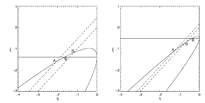
Figure 13: The asymmetric curve corresponds to a local maximum for all points on the segment from $A$ (where it crosses the line $\widetilde{\xi}=\widetilde{\eta}+4/3\beta^{2}$) to $B$ (where it crosses $\widetilde{\xi}=-4/\beta^{2}$ and becomes unphysical. It is the global maximum only in the region below the diagonal, which it crosses at $D$. If $\beta<2$, $D$ lies above $B$ so the asymmetric configuration is never a global maximum. If $\beta>2$ then the asymmetric configuration is the global maximum for every point on the segment between $D$ and $B$.

The regions of symmetric and asymmetric upper thresholds thus take the form shown in Figure 6. The the boundary of the lens shaped region next to the diagonal is determined by the curve (71) consisting of the points where the symmetric and asymmetric segements join. The bottom of the lens meets the diagonal at the $\beta=2$ line.

References

- (1) Galileo Galilei, Dialogo sopra i due massimi sistemi del mondo, (“Dialog concerning the two chief world systems”), second day.
-
(2)
C. J. Isham, “Structural issues in quantum gravity”,
[arXiv:gr-qc/9510063];
J. Butterfield and C. J. Isham, “On the emergence of time in quantum gravity”, [arXiv:gr-qc/9901024]. - (3) K. V. Kuchar, “Time And Interpretations Of Quantum Gravity”, In “Winnipeg 1991, Proceedings, General relativity and relativistic astrophysics”, 211-314.
- (4) V. A. Kostelecky and S. Samuel, Phys. Rev. D 39, 683 (1989).
-
(5)
R. Gambini and J. Pullin,
Phys. Rev. D 59, 124021 (1999);
J. Alfaro, H. A. Morales-Tecotl and L. F. Urrutia, Phys. Rev. Lett. 84, 2318 (2000);
J. Alfaro, H. A. Morales-Tecotl and L. F. Urrutia, Phys. Rev. D 65, 103509 (2002). -
(6)
M. Hayakawa,
Phys. Lett. B 478, 394 (2000)
[arXiv:hep-th/9912094];
M. Hayakawa, arXiv:hep-th/9912167. - (7) S. M. Carroll, J. A. Harvey, V. A. Kostelecky, C. D. Lane and T. Okamoto, Phys. Rev. Lett. 87, 141601 (2001).
- (8) G. Amelino-Camelia, L. Doplicher, S. Nam and Y. S. Seo, arXiv:hep-th/0109191.
- (9) R. J. Protheroe and H. Meyer, Phys. Lett. B 493, 1 (2000).
- (10) K. Greisen, Phys. Rev. Lett. 16, 748 (1996).
- (11) G.T. Zatsepin and V.A. kuz’min, Zh. Eksp. Teor. Fiz., Pis’ma Red. 4, 114 (1966) [JETP lett. 4, 78 (1966).
- (12) F. Stecker, Phys. Rev. Lett. 21, 1016 (1968).
-
(13)
N. Hayashida et al., Phys. Rev. Lett. 73, 3491 (1994);
Haverah Park Collaboration, M.A. Lawrence et al., J. Phys. G 17,733 (1991);
S. Yoshida et al., Astropart. Phys. 3, 105 (1995);
Fly’s Eye collaboration, D.J. Bird et al., Astrophys. J. 424, 144 (1995);
M. Takeda et al., Phys. Rev. Lett. 81, 1163 (1998). - (14) M. Nagano, A. A. Watson, Rev. Mod. Phys.72, 689 (2000).
-
(15)
G. Sigl,
Lect. Notes Phys. 556, 259 (2000);
G. Sigl, Science 291, 73 (2001). - (16) F. W. Stecker, arXiv:astro-ph/0208507.
- (17) S. Coleman and S. L. Glashow, Phys. Rev. D 59, 116008 (1999).
-
(18)
L. Gonzalez-Mestres, ‘‘Deformed Lorentz symmetry and
high-energy astrophysics. I”, [arXiv:physics/0003080];
L. Gonzalez-Mestres, ‘‘Physical and cosmological implications of a possible class of particles able to travel faster than light”, [arXiv:hep-ph/9610474];
L. Gonzalez-Mestres, ‘‘Properties of a possible class of particles able to travel faster than light”, [arXiv:astro-ph/9505117]. -
(19)
O. Bertolami,
Gen. Rel. Grav. 34, 707 (2002);
O. Bertolami, Nucl. Phys. Proc. Suppl. 88, 49 (2000);
O. Bertolami and C. S. Carvalho, Phys. Rev. D 61, 103002 (2000). -
(20)
G. Amelino-Camelia and T. Piran,
Phys. Lett. B 497, 265 (2001);
G. Amelino-Camelia and T. Piran, Phys. Rev. D 64, 036005 (2001);
G. Amelino-Camelia, Phys. Lett. B 528, 181 (2002). - (21) O. C. de Jager and F. W. Stecker, Astrophys. J. 566, 738 (2002)
- (22) J. N. Bahcall and E. Waxman, “Has the GZK cutoff been discovered?”, [arXiv:hep-ph/0206217].
- (23) The High Resolution Fly’s Eye Collaboration, Measurement of the Spectrum of UHE Cosmic Rays by the FADC Detector of the HiRes Experiment, [arXiv:astro-ph/0208301].
-
(24)
G. Amelino-Camelia, J. R. Ellis, N. E. Mavromatos,
D. V. Nanopoulos and S. Sarkar, “Sensitivity of
astrophysical observations to gravity-induced wave dispersion in
vacuo”, [astro-ph/9810483];
G. Amelino-Camelia, J. R. Ellis, N. E. Mavromatos, D. V. Nanopoulos and S. Sarkar, Nature 393, 763 (1998). -
(25)
W. Kluźniak,
Astropart. Phys. 11, 117 (1999);
W. Kluzniak, “Is the universe transparent to TeV photons?”, [arXiv:astro-ph/9905308]. - (26) T. Kifune, Astrophys. J. 518, L21 (1999).
- (27) R. Aloisio, P. Blasi, P. L. Ghia and A. F. Grillo, Phys. Rev. D 62, 053010 (2000).
- (28) T. Jacobson, S. Liberati and D. Mattingly, “TeV astrophysics constraints on Planck scale Lorentz violation”, [arXiv:hep-ph/0112207]. To appear in Rapid. Comm. PRD.
- (29) T. J. Konopka and S. A. Major, New J. Phys. 4, 57 (2002).
-
(30)
D. Colladay and V. A. Kostelecky,
Phys. Rev. D 55, 6760 (1997);
D. Colladay and V. A. Kostelecky, Phys. Rev. D 58, 116002 (1998). - (31) J. R. Ellis, N. E. Mavromatos and D. V. Nanopoulos, Phys. Rev. D 63, 124025 (2001).
- (32) Y. J. Ng and H. Van Dam, Mod. Phys. Lett. A 9, 335 (1994).
- (33) T. Jacobson, Prog. Theor. Phys. Suppl. 136, 1 (1999).
- (34) J. C. Niemeyer, [arXiv:astro-ph/0201511].
- (35) J. C. Niemeyer, R. Parentani and D. Campo, Phys. Rev. D 66, 083510 (2002).
- (36) R. H. Brandenberger, “Trans-Planckian physics and inflationary cosmology”, [arXiv:hep-th/0210186].
- (37) C. P. Burgess, J. Cline, E. Filotas, J. Matias and G. D. Moore, JHEP 0203, 043 (2002) [arXiv:hep-ph/0201082].
-
(38)
V. A. Kostelecky, “Theory and tests of CPT and Lorentz
violation”, [arXiv:hep-ph/9904467];
Ibidem, Proceedings of the “Second Meeting on CPT and Lorentz Symmetry”, Bloomington, Usa, 15-18 August 2001”. Singapore, World Scientific (2002). - (39) V. A. Kostelecky and M. Mewes, Phys. Rev. Lett. 87, 251304 (2001)
- (40) F. W. Stecker and S. L. Glashow, Astropart. Phys. 16, 97 (2001).
- (41) G. Amelino-Camelia, Phys. Lett. B 510, 255 (2001); Int. J. Mod. Phys. D 11, 35 (2002).
- (42) J. Kowalski-Glikman and S. Nowak, Phys. Lett. B 539, 126 (2002).
- (43) J. Magueijo and L. Smolin, Phys. Rev. Lett. 88, 190403 (2002) [arXiv:hep-th/0112090].
- (44) S. Judes and M. Visser, [arXiv:gr-qc/0205067].
- (45) V. A. Kostelecky and R. Lehnert, Phys. Rev. D 63, 065008 (2001).
- (46) V. A. Kostelecky and S. Samuel, Phys. Rev. D 40, 1886 (1989).
- (47) S. M. Carroll, G. B. Field and R. Jackiw, Phys. Rev. D 41, 1231 (1990).
-
(48)
M. Gasperini,
Class. Quant. Grav. 4, 485 (1987);
M. Gasperini, Gen. Rel. Grav. 30, 1703 (1998). -
(49)
T. Jacobson and D. Mattingly,
Phys. Rev. D 63, 041502 (2001).
T. Jacobson and D. Mattingly, Phys. Rev. D 64, 024028 (2001). - (50) R. J. Gleiser and C. N. Kozameh, Phys. Rev. D 64, 083007 (2001).
- (51) R. N. Mohapatra and P. B. Pal, “Massive Neutrinos In Physics And Astrophysics. Second Edition”, World Sci. Lect. Notes Phys. 60, 1 (1998). See Chapter 11, p. 195.
- (52) B. A. Bassett, S. Liberati, C. Molina-Paris and M. Visser, Phys. Rev. D 62, 103518 (2000).
- (53) G. D. Moore and A. E. Nelson, JHEP 0109, 023 (2001).
- (54) S. Coleman and S. L. Glashow, Phys. Lett. B 405, 249 (1997).
- (55) V. D. Barger, S. Pakvasa, T. J. Weiler and K. Whisnant, Phys. Rev. Lett. 85, 5055 (2000).
- (56) R. Brustein, D. Eichler and S. Foffa, Phys. Rev. D 65, 105006 (2002).
- (57) D. Sudarsky, L. Urrutia and H. Vucetich, “New observational bounds to quantum gravity signals”, [arXiv:gr-qc/0204027].
- (58) K. Koyama, R. Petre, E.V. Gotthelf, U. Hwang, M. Natsuura, M. Ozaki, and S.S. Holt, Nature 378, 255 (1995).
- (59) T. Naito, T. Yoshida, M. Mori, T. Tanimori, Astronomische Nachrichten 320, 205 (1999).
- (60) T. Jacobson, S. Liberati and D. Mattingly, “Lorentz violation and Crab synchrotron emission: A new constraint far beyond the Planck scale”, [arXiv:astro-ph/0212190].
- (61) T. Tanimori et al., ApJ 492, L33 (1998).
- (62) D. Mattingly, T. Jacobson and S. Liberati, Phys. Rev. D 67, 124012 (2003)
- (63) J. Nishimura et al., Proceedings of the 25th Int. Cosmic-Ray Conf. (Durban), 4, 233.
- (64) F.A. Aharonian, A.M. Atoian and T. Kifune, Mon. Note. R. Astron, Soc. 291, 162-176 (1997).
- (65) F. Krennrich et al., Astrophys. J. 560 (2001) L45
-
(66)
F. A. Aharonian, A&A 349, 11 (1999);
F. A. Aharonian and P. S. Coppi, Astropart. Phys. 11, 35 (1999). - (67) F. A. Aharonian, A. N. Timokhin and A. V. Plyasheshnikov, “On the origin of highest energy gamma-rays from Mkn-501”, [arXiv:astro-ph/0108419].
- (68) A. K. Konopelko, A. Mastichiadis, J. G. Kirk, O. C. de Jager and F. W. Stecker, “Modelling the TeV gamma-ray spectra of two low redshift AGNs: Mkn 501 and Mkn 421”, [arXiv:astro-ph/0302049].
- (69) T. Jacobson, S. Liberati and D. Mattingly, “Comments on ’Improved limit on quantum-spacetime modifications of Lorentz symmetry from observations of gamma-ray blazars’ ”, [arXiv:gr-qc/0303001].
- (70) J. R. Ellis, K. Farakos, N. E. Mavromatos, V. A. Mitsou and D. V. Nanopoulos, Astrophys. J. 535, 139 (2000).
- (71) T.G. Pavlopoulos, Breakdown of Lorentz invariance, Phys. Rev. 159, 1106 (1967).
- (72) S. Sarkar, Mod. Phys. Lett. A 17, 1025 (2002).
- (73) S. D. Biller et al., Phys. Rev. Lett. 83, 2108 (1999).
- (74) M. Sommer et al., “High-energy gamma rays from the intense 1993 January 31 gamma-ray burst”, Ap. J. 422, L63 (1994).
- (75) B. Schaefer, “Severe Limits on Variations of the Speed of Light with Frequency”, Phys. Rev. Lett. 82, 4964 (1999).
- (76) J. P. Norris, J. T. Bonnell, G. F. Marani and J. D. Scargle, “GLAST, GRBs, and quantum gravity”, [arXiv:astro-ph/9912136].
- (77) V. A. Kostelecky, C. D. Lane and A. G. Pickering, Phys. Rev. D 65, 056006 (2002).
- (78) M. Messier, Evidence for neutrino mass from observations of atmospheric neutrino with Super Kamiokande, Ph.D. Thesis, Boston University, 1999.
- (79) J. Ahrens et al. [AMANDA Collaboration], Phys. Rev. D 66, 012005 (2002)
-
(80)
T. Miller et al., ‘‘From AMANDA to IceCube: Current
and future high energy neutrino telescopes at the South Pole”.
Published in the Proceedings of “Baltimore 1999, Neutrinos in the
new millennium”, pg. 47-61. Edited by G. Domokos, S.
Kovesi-Domokos. Singapore, World Scientific, 2000.
C. Spiering [AMANDA Collaboration], Annalen Phys. 10, 131 (2001). - (81) F. W. Stecker, Astrophys. J. 228, 919 (1979).
- (82) http://area51.berkeley.edu/manuscripts/nu2002/nu2002-uhenu.pdf
- (83) A. Kusenko and T. J. Weiler, Phys. Rev. Lett. 88, 161101 (2002).
- (84) J. L. Feng, P. Fisher, F. Wilczek and T. M. Yu, Phys. Rev. Lett. 88, 161102 (2002).
- (85) D. De Marco, P. Blasi and A. V. Olinto, “On the statistical significance of the GZK feature in the spectrum of ultra high energy cosmic rays”, [arXiv:astro-ph/0301497].