Calculation of Hadronic Excitations of the Quark-Gluon Plasma

Abstract

We present calculations of the spectral functions of various hadronic current correlators at finite temperature, making use of the Nambu–Jona-Lasinio (NJL) model and the real-time finite-temperature formalism. We study the scalar-isoscalar correlation function in a SU(3)-flavor model, as well as the pseudoscalar and vector correlation functions. We relate our analysis to our recent calculations of the properties of mesons for $T<T_{c}$, which made use of a generalized NJL model that includes a covariant model of confinement. Here, we exhibit values of the spectral functions for a range of values of $T>T_{c}$, where it is possible to neglect the effects of confinement. We find important excitations in the scalar sector corresponding to what are predominately singlet and octet states. The singlet state, which is at 550 MeV at $T=1.2\,T_{c}$, evolves from the $f_{0}(980)$ which has an energy of about 400 MeV before it disappears from the spectrum of bound states for $T>0.95\,T_{c}$. The octet state seen at $T=1.2\,T_{c}$, which has a mass of about 1100 MeV, evolves from a nodeless state that has an energy of about 1470 MeV at $T=0$ in our model. As noted in the literature, these modes may play an important role in the cooling and hadronization of quark-gluon droplets excited in heavy-ion collisions. In the past, those researchers who have used the SU(2)-flavor version of the NJL (without confinement) and the imaginary-time formalism have found bound states for the sigma and pion for temperatures that are larger than $T_{c}$. In those works it is seen that the sigma and pion become degenerate after the restoration of chiral symmetry, as that restoration described in the NJL model. The energy of that mode then increases with increasing temperature. Our model, however, has several advantages over previous studies. We are able to describe meson properties below $T_{c}$, as well as the confinement-deconfinement transition. Then, using the real-time formalism, we are able to describe the widths of the excitations of the quark gluon plasma that evolve from the pion and $f_{0}(980)$ with increasing temperature.

I INTRODUCTION

Some years ago it was suggested that the quark-gluon plasma was a “confining medium” in the sense that the important excitations should be color singlets [1]. At about the same time, Hatsuda and Kunihiro reported a study of “soft modes” of the quark-gluon plasma [2]. These authors used a SU(2)-flavor version of the Nambu–Jona-Lasinio (NJL) model [3] and considered both finite temperature and density, making use of the Matsubara imaginary-time formalism [4,5]. (The standard NJL model does not describe confinement, so that the question arises as to the modifications of the results obtained in Ref. [2] if a model of confinement were to be included.) In Ref. [2] it was found that the sigma meson mass, which lies in the continuum of the model, begins to drop in energy with increasing temperature, while the pion energy increases (slowly) with increasing temperature. Eventually, the sigma and pion become degenerate in energy, with the resulting mode increasing in energy with increasing temperature. These results have been confirmed in a very detailed recent study making use of a field-theoretic approach in the calculation of the pseudoscalar and scalar correlation functions at finite temperature [6]. In that work, phenomenological forms for the nonperturbative features of the gluon propagator were introduced and the Schwinger-Dyson and Bethe-Salpeter equations were solved. In many cases, the model of Ref. [6] yields results that are similar to those obtained when using the NJL model. It is of interest to compare the results of our present study with those obtained in Ref. [6] and to note some of the differences between our SU(3)-flavor analysis and the SU(2)-flavor analysis of Ref. [6]. We will return to a discussion of the results obtained in our work and those obtained in Ref. [6] in Section VI.

Recently, we have also seen an extensive effort in the calculation of hadronic correlation functions using lattice simulation of QCD at finite temperature [7-9]. These calculations make use of the maximum entropy method (MEM) which is reviewed in Ref. [10]. Various peaks are seen in the spectral functions for $T<T_{c}$ which persist for $T>T_{c}$. It is only at relatively large values of $T$ that the correlation functions go over to the smooth behavior expected for a weakly interacting system [7-9].

Although we have introduced a critical temperature for the purposes of our discussion, we should note that the quark masses and vacuum condensates do not go to precisely zero at large temperature, since the current quark mass is always present in the model. Indeed, the presence of a small current mass, $m_{u}^{0}=0.0055$ GeV, makes for a significant change in the behavior of $m_{u}(T)$ with increasing temperature. On the other hand, it is useful to introduce a value of $T_{c}$ of the order of 170 MeV to facilitate the discussion. The significance of that value for the characterization of the constituent mass of the up (or down) quark may be inferred from Fig. 1, which exhibits results calculated for $m_{u}^{0}=0.0055$ GeV and $m_{s}^{0}=0.120$ GeV.

Figure 1: Temperature-dependent constituent mass values, $m_{u}(T)$ and $m_{s}(T)$, calculated in a mean-field approximation [12] are shown. [See Eq. (2.2)]. Here $m_{u}^{0}=0.0055$ GeV, $m_{s}^{0}=0.120$ GeV, and $G(T)=5.691[1-0.17(T/T_{c})]$ GeV², if we use Klevansky’s notation [12]. (The value of $G$ used in our work is defined such that it is twice the value of $G$ used in Ref. [12].)

It is of interest to obtain insight into the lattice results for spectral functions by studying hadronic current correlators in a model, such as the NJL model, that describes the restoration of chiral symmetry with increasing temperature. We present such a study in this work. The organization of our work is as follows. In Section II we review our model of confinement and our calculations of meson properties for $T<T_{c}$. In Section III we describe the calculation of the imaginary part of the vacuum polarization function of the NJL model, when use is made of the real-time finite-temperature formalism. Once the imaginary part is calculated, the real part may be obtained using a dispersion relation. In Section IV we show how hadronic current correlation functions may be constructed in terms of the vacuum polarization functions calculated in Section III. In Section V we present results of numerical calculations of the various hadronic current correlation functions considered in this work. Finally, Section VI contains some further discussion and some comparison of the Minkowski-space analysis of the present work and the Euclidean-space analysis of Ref. [6].

II calculation of meson properties at finite temperature in a generalized NJL model with confinement

It is useful to record the Lagrangian used in our calculations of meson properties

$${\cal L}= \bar{q}(i\hbox to0.0pt{\hbox to5.30904pt{\hfil/\hfil}\hss}\partial-m^{0})q+\frac{G_{S}}{2}\sum_{i=0}^{8}[(\bar{q}\lambda^{i}q)^{2}+(\bar{q}i\gamma_{5}\lambda^{i}q)^{2}]$$ (2.1)

$$-\frac{G_{V}}{2}\sum_{i=0}^{8}[(\bar{q}\lambda^{i}\gamma_{\mu}q)^{2}+(\bar{q}\lambda^{i}\gamma_{5}\gamma_{\mu}q)^{2}]$$

$$+\frac{G_{D}}{2}\{\det[\bar{q}(1+\gamma_{5})q]+\det[\bar{q}(1-\gamma_{5})q]\}$$

$$+{\cal L}_{conf}\,,$$

Here, $m^{0}$ is a current quark mass matrix, $m^{0}=\mbox{diag}\,(m_{u}^{0},\,m_{d}^{0},\,m_{s}^{0})$. The $\lambda^{i}$ are the Gell-Mann (flavor) matrices, $\lambda^{0}=\sqrt{2/3}\mathbf{\,1}$ with $\mathbf{\,1}$ being the unit matrix. The fourth term on the right-hand side of Eq. (2.1) is the ’t Hooft interaction. Finally, ${\cal L}_{conf}$ represents the model of confinement we have used in our work.

As noted earlier, we have recently reported results of our calculations of the temperature dependence of the spectra of various mesons [11]. These calculations were made using our generalized NJL model which includes a covariant model of confinement. We have presented results for the $\pi$, $K$, $a_{0}$, $f_{0}$ and $K_{0}^{*}$ mesons in Ref. [11].

There are three important temperature-dependent features of our model. Temperature-dependent constituent quark masses were calculated using the equation [12]

$$m(T)=m^{0}+2G_{S}(T)N_{c}\frac{m(T)}{\pi^{2}}+\int_{0}^{\Lambda}dp\frac{P^{2}}{E_{p}}\tanh(\frac{1}{2}\beta E_{p})\,.$$ (2.2)

Here, $m^{0}$ is the current quark mass, $G_{S}(T)$ is a temperature-dependent coupling constant introduced in our model [11]

$$G_{S}(T)=G_{S}\left[1-0.17\left(\frac{T}{T_{c}}\right)\right]\,,$$ (2.3)

$N_{c}=3$ is the number of colors, $\beta=1/T$ and $E_{p}=\left[\vec{p}\;{}^{2}+m^{2}(T)\right]^{1/2}$. Further, $\Lambda=0.631$ GeV is a cutoff such that $|\vec{p}|\leq\Lambda$. Results obtained for the up (or down) and strange quark masses are given in Fig. 1. In calculating the constituent mass values we have neglected the confining interaction. That interaction was taken into account in our earlier Euclidean-space calculation of the quark self-energy [13], which also included the effects related to ’t Hooft interaction. We found that, to a good approximation, we could neglect the confining and ’t Hooft interactions, if we modified the value of the NJL coupling constant, $G_{S}$, and we adopt that approach when using Eq. (2.2).

In addition to the temperature dependence of the coupling constant and constituent mass values, we also introduced a temperature-dependent confining potential, whose form was motivated by recent lattice simulations of QCD in which the temperature dependence of the confining interaction was calculated with dynamical quarks [14]. (See Fig. 2.) In order to include such effects, we modified the form of our confining interaction, $V^{C}(r)=\kappa r\exp[-\mu r]$, by replacing $\mu$ by

$$\mu(T)=\frac{\mu_{0}}{\left[1-0.7\left(\displaystyle\frac{T}{T_{c}}\right)^{2}\right]}\,,$$ (2.4)

with $\mu_{0}=0.010$ GeV. The maximum value of $V^{C}(r,T)$ is then

$$V_{max}^{C}(T) = \frac{\kappa}{\mu(T)e}\,,$$ (2.5)

$$= \frac{\kappa\left[1-0.7({T}/{T_{c}})^{2}\right]}{\mu_{0}e}\,,$$ (2.6)

with $r_{max}=1/\mu(T)$. To better represent the qualitative features of the results shown in Fig. 2, we can use $V^{C}(r,T)=\kappa r\exp[-\mu(T)r]$ for $r\leq r_{max}$ and $V^{C}(r,T)=V_{max}^{C}(T)$ for $r>r_{max}$. We also note that we use Lorentz-vector confinement and carry out all our calculations in momentum-space. The value of $\kappa$ used in our work is 0.055 GeV².

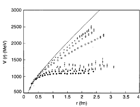
Figure 2: A comparison of quenched (open symbols) and unquenched (filled symbols) results for the interquark potential at finite temperature [14]. The dotted line is the zero temperature quenched potential. Here, the symbols for $T=0.80T_{c}$ [open triangle], $T=0.88T_{c}$ [open circle], $T=0.80T_{c}$ [open square], represent the quenched results. The results with dynamical fermions are given at $T=0.68T_{c}$ [solid downward-pointing triangle], $T=0.80T_{c}$ [solid upward-pointing triangle], $T=0.88T_{c}$ [solid circle], and $T=0.94T_{c}$ [solid square].

We do not attempt to review the details of our calculations of temperature-dependent meson spectra [11]. However, in Figs. 3 and 4 we show the results for the $\pi$ and $f_{0}$ mesons obtained in Ref. [11]. (These calculations were made with the temperature-dependent potentials shown in Fig. 5.) In Figs. 3 and 4, it may be seen that, as $T\rightarrow T_{c}$, fewer states are bound, with no bound states remaining at $T=T_{c}$ . Our confining potential is finite at $T=T_{c}$ , but has a zero value for $T=1.195T_{c}$ . (The potential is defined to be equal to zero for $T\geq 1.195T_{c}$ .) However, it is important to note that $G_{S}(T)=0$ only for the quite large value $T=5.88T_{c}$ . (The coupling constants of the model are taken to be zero for $T\geq 5.88T_{c}$ .) Even though the confining potential is absent for $T\geq 1.2T_{c}$ , the continued presence of the short-range NJL interaction has important consequences for the dynamics of the quark-gluon plasma, as we will explore in the following sections.

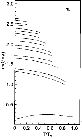
Figure 3: The mass values of the pionic states calculated in Ref. [11] with $G_{\pi}(T)=13.49[1-0.17\,T/T_{c}]$ GeV^-2, $G_{V}(T)=11.46[1-0.17\,T/T_{c}]$ GeV^-2, and the quark mass values given in Fig. 1. The value of the pion mass is 0.223 GeV at $T/T_{c}=0.90$, where $m_{u}(T)=0.102$ GeV and $m_{s}(T)=0.449$ GeV.

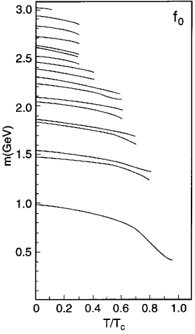
Figure 4: Mass values of the $f_{0}$ mesons calculated in Ref. [11] with $G_{00}(T)=14.25[1-0.17\,T/T_{c}]$ GeV^-2, $G_{88}(T)=10.65[1-0.17\,T/T_{c}]$ GeV^-2, $G_{08}(T)=0.495[1-0.17\,T/T_{c}]$ GeV^-2, and $G_{80}(T)=G_{08}(T)$ in a singlet-octet representation. The quark mass values used are shown in Fig. 1. The $f_{0}$ has a mass of 0.400 GeV at $T/T_{c}=0.95$.

Figure 5: The potential $V^{C}(r,T)$ is shown for $T/T_{c}=0$ [solid line], $T/T_{c}=0.4$ [dotted line], $T/T_{c}=0.6$ [dashed line], $T/T_{c}=0.8$ [dashed-dotted line], $T/T_{c}=0.9$ [short dashes], $T/T_{c}=1.0$ [dashed-(double) dotted line]. Here, $V^{C}(r,T)=\kappa r\exp[-\mu(T)r]$, with $\mu(T)=0.01\mbox{GeV}/[1-0.7(T/T_{c})^{2}]$ and $\kappa=0.055$ GeV².

III polarization functions at finite temperature

The basic polarization functions that are calculated in the NJL model are shown in Fig. 6. We will consider calculations of such functions in the frame where $\vec{P}=0$. In our earlier work, calculations were made after a confinement vertex was included. That vertex is represented by the filled triangular region in Fig. 6. However, we here consider calculations for $T\geq 1.2T_{c}$ where confinement may be neglected. We will, however, use the temperature-dependent mass values shown in Fig. 1.

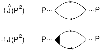
Figure 6: The upper figure represents the basic polarization diagram of the NJL model in which the lines represent a constituent quark and a constituent antiquark. The lower figure shows a confinement vertex [filled triangular region] used in our earlier work. For the present work we neglect confinement for $T\geq 1.2T_{c}$, with $T_{c}=170$ MeV.

The procedure we adopt is based upon the real-time finite-temperature formalism, in which the imaginary part of the polarization function may be calculated. Then, the real part of the function is obtained using a dispersion relation. The result we need for this work has been already given in the work of Kobes and Semenoff [15]. (In Ref. [15] the quark momentum in Fig. 6 is $k$ and the antiquark momentum is $k-P$. We will adopt that notation in this section for ease of reference to the results presented in Ref. [15].) With reference to Eq. (5.4) of Ref. [15], we write the imaginary part of the scalar polarization function as

$$\mbox{Im}\,J^{S}(\textit{P}\,{}^{2},T)=\frac{1}{2}(2N_{C})\beta_{S}\,\epsilon(\textit{P}\,{}^{0})\!\int\!\!\frac{d^{3}\!{k}}{(2\pi)^{3}}\,e^{-\vec{k}\,{}^{2}/\alpha^{2}}\left(\frac{2\pi}{2E_{1}(k)2E_{2}(k)}\right)$$ (3.1)

$$\{(1-n_{1}(k)-n_{2}(k))\delta(\textit{P}\,{}^{0}-E_{1}(k)-E_{2}(k))$$

$$-(n_{1}(k)-n_{2}(k))\delta(\textit{P}\,{}^{0}+E_{1}(k)-E_{2}(k))$$

$$-(n_{2}(k)-n_{1}(k))\delta(\textit{P}\,{}^{0}-E_{1}(k)+E_{2}(k))$$

$$-(1-n_{1}(k)-n_{2}(k))\delta(\textit{P}\,{}^{0}+E_{1}(k)+E_{2}(k))\}\,.$$

Here, $E_{1}(k)=[\vec{k}\,{}^{2}+m_{1}^{2}(T)]^{1/2}$. Relative to Eq. (5.4) of Ref. [15], we have changed the sign, removed a factor of $g^{2}$ and have included a statistical factor of $2N_{C}$, where the factor of 2 arises from the flavor trace. In addition, we have included a Gaussian regulator, $\exp[-\vec{k}\,{}^{2}/\alpha^{2}]$, with $\alpha=0.605$ GeV, which is the same as that used in most of our applications of the NJL model in the calculation of meson properties [16-21]. We also note that

$$n_{1}(k)=\frac{1}{e^{\,\beta E_{1}(k)}+1}\,,$$ (3.2)

and

$$n_{2}(k)=\frac{1}{e^{\,\beta E_{2}(k)}+1}\,.$$ (3.3)

For the calculation of the imaginary part of the polarization function, we may put $k^{2}=m_{1}^{2}(T)$ and $(k-P)^{2}=m_{2}^{2}(T)$, since in that calculation the quark and antiquark are on-mass-shell. In Eq. (3.1) the factor $\beta_{S}$ arises from a trace involving Dirac matrices, such that

$$\beta_{S} = -\mbox{Tr}[(\hbox to0.0pt{\hbox to5.52084pt{\hfil/\hfil}\hss}k+m_{1})(\hbox to0.0pt{\hbox to5.52084pt{\hfil/\hfil}\hss}k-\hbox to0.0pt{\hbox to7.80904pt{\hfil/\hfil}\hss}P+m_{2})]$$ (3.4)

$$= 2P^{2}-2(m_{1}+m_{2})^{2}\,,$$ (3.5)

where $m_{1}$ and $m_{2}$ depend upon temperature. In the frame where $\vec{P}=0$, and in the case $m_{1}=m_{2}$, we have $\beta_{S}=2P_{0}^{2}(1-{4m^{2}}/{P_{0}^{2}})$. For the scalar case, with $m_{1}=m_{2}$, we find

$$\mbox{Im}\,J^{S}(P^{2},T)=\frac{N_{c}P_{0}^{2}}{4\pi}\left(1-\frac{4m^{2}}{P_{0}^{2}}\right)^{3/2}e^{-\vec{k}\,{}^{2}/\alpha^{2}}[1-2n_{1}(k)]\,,$$ (3.6)

where

$$\vec{k}\,{}^{2}=\frac{P_{0}^{2}}{4}-m^{2}(T)\,.$$ (3.7)

We may evaluate Eq. (3.6) for $m(T)=m_{u}(T)=m_{d}(T)$ and define $\mbox{Im}\,J_{u}^{S}(P^{2},T)$. When we put $m(T)=m_{s}(T)$, we define $\mbox{Im}\,J_{s}^{S}(P^{2},T)$. These two functions will be needed for our calculation of the scalar-isoscalar correlator discussed in the next section. The real parts of the functions $J_{u}^{S}(P^{2},T)$ and $J_{s}^{S}(P^{2},T)$ may be obtained using a dispersion relation, as noted earlier.

For pseudoscalar mesons, we replace $\beta_{S}$ by

$$\beta_{P} = -\mbox{Tr}[i\gamma_{5}(\hbox to0.0pt{\hbox to5.52084pt{\hfil/\hfil}\hss}k+m_{1})i\gamma_{5}(\hbox to0.0pt{\hbox to5.52084pt{\hfil/\hfil}\hss}k-\hbox to0.0pt{\hbox to7.80904pt{\hfil/\hfil}\hss}P+m_{2})]$$ (3.8)

$$= 2P^{2}-2(m_{1}-m_{2})^{2}\,,$$ (3.9)

which for $m_{1}=m_{2}$ is $\beta_{P}=2P_{0}^{2}$ in the frame where $\vec{P}=0$. We find, for the $\pi$ mesons,

$$\mbox{Im}\,J^{P}(P^{2},T)=\frac{N_{c}P_{0}^{2}}{4\pi}\left(1-\frac{4m(T)^{2}}{P_{0}^{2}}\right)^{1/2}e^{-\vec{k}\,{}^{2}/\alpha^{2}}[1-2n_{1}(k)]\,,$$ (3.10)

where $\vec{k}\,{}^{2}={P_{0}^{2}}/4-m_{u}^{2}(T)$, as above. Thus, we see that, relative to the scalar case, the phase space factor has an exponent of 1/2 corresponding to a s-wave amplitude. For the scalars, the exponent of the phase-space factor is 3/2, as seen in Eq. (3.6).

For a study of vector mesons we consider

$$\beta_{\mu\nu}^{V}=\mbox{Tr}[\gamma_{\mu}(\hbox to0.0pt{\hbox to5.52084pt{\hfil/\hfil}\hss}k+m_{1})\gamma_{\nu}(\hbox to0.0pt{\hbox to5.52084pt{\hfil/\hfil}\hss}k-\hbox to0.0pt{\hbox to7.80904pt{\hfil/\hfil}\hss}P+m_{2})]\,,$$ (3.11)

and calculate

$$g^{\mu\nu}\beta_{\mu\nu}^{V}=4[P^{2}-m_{1}^{2}-m_{2}^{2}+4m_{1}m_{2}]\,,$$ (3.12)

which, in the equal-mass case, is equal to $4P_{0}^{2}+8m^{2}(T)$, when $m_{1}=m_{2}$ and $\vec{P}=0$. This result will be needed when we calculate the correlator of vector currents in the next section. Note that for the elevated temperatures considered in this work $m_{u}(T)=m_{d}(T)$ is quite small, so that $4P_{0}^{2}+8m_{u}^{2}(T)$ can be approximated by $4P_{0}^{2}$ when we consider the $\rho$ meson.

IV calculation of hadronic current correlation functions

In this section we consider the calculation of temperature-dependent hadronic current correlation functions. The general form of the correlator is a transform of a time-ordered product of currents,

$$iC(P^{2},T)=\int d^{4}xe^{\,iP\cdot x}<<\mbox{T}(j(x)j(0)>>\,,$$ (4.1)

where the double bracket is a reminder that we are considering the finite temperature case.

For the study of pseudoscalar states, we may consider currents of the form $j_{P,\,i}(x)=\bar{q}(x)i\gamma_{5}\lambda^{i}q(x)$, where, in the case of the $\pi$ mesons, $i=1,2,$ and 3. For the study of scalar-isoscalar mesons, we introduce $j_{S,\,i}(x)=\bar{q}(x)\lambda^{i}q(x)$, where $i=0$ for the flavor-singlet current and $i=8$ for the flavor-octet current.

In the case of the $\pi$ mesons, the correlator may be expressed in terms of the basic vacuum polarization function of the NJL model, $J_{P}(P^{2},T)$ [12, 22, 23]. Thus,

$$C_{\pi}(P^{2},T)=J_{P}(P^{2},T)\frac{1}{1-G_{\pi}(T)J_{P}(P^{2},T)}\,,$$ (4.2)

where $G_{\pi}(T)$ is the coupling constant appropriate for our study of the $\pi$ mesons. We have found $G_{\pi}(0)=13.51$ GeV^-2 by fitting the pion mass in a calculation made at $T=0$, with $m_{u}=m_{d}=0.364$ GeV [11]. (We will describe the calculation of $J_{P}(P^{2},T)$ later in this section.)

The calculation of the correlator for scalar-isoscalar states is more complex, since there are both flavor-singlet and flavor-octet states to consider. We may define polarization functions for $u$, $d$ and $s$ quarks: $J_{u}(P^{2},T)$, $J_{d}(P^{2},T)$ and $J_{s}(P^{2},T)$. (These functions do not contain the factor of 2 that would otherwise appear when forming the flavor trace.) In terms of these polarization functions we may then define

$$J_{00}(P^{2},T)=\frac{2}{3}[J_{u}(P^{2},T)+J_{d}(P^{2},T)+J_{s}(P^{2},T)]\,,$$ (4.3)

$$J_{08}(P^{2},T)=\frac{\sqrt{2}}{3}[J_{u}(P^{2},T)+J_{d}(P^{2},T)-2J_{s}(P^{2},T)]\,,$$ (4.4)

and

$$J_{88}(P^{2},T)=\frac{1}{3}[J_{u}(P^{2},T)+J_{d}(P^{2},T)+4J_{s}(P^{2},T)]\,.$$ (4.5)

We also introduce the matrices

$$J(P^{2},T)=\left[\begin{array}[]{cc}J_{00}(P^{2},T)&J_{08}(P^{2},T)\\ J_{80}(P^{2},T)&J_{88}(P^{2},T)\end{array}\right]\,,$$ (4.8)

$$G(T)=\left[\begin{array}[]{cc}G_{00}(T)&G_{08}(T)\\ G_{80}(T)&G_{88}(T)\end{array}\right]\,,$$ (4.11)

and

$$C(P^{2},T)=\left[\begin{array}[]{cc}C_{00}(P^{2},T)&C_{08}(P^{2},T)\\ C_{80}(P^{2},T)&C_{88}(P^{2},T)\end{array}\right]\,.$$ (4.14)

We then write the matrix relation

$$C(P^{2},T)=J(P^{2},T)[1-G(T)J(P^{2},T)]^{-1}\,.$$ (4.15)

For some purposes it may be useful to also define a t matrix

$$t(P^{2},T)=[1-G(T)J(P^{2},T)]^{-1}G(T)\,,$$ (4.16)

where $t(P^{2},T)$ has the structure shown in Eqs. (4.6)-(4.8). The same resonant structures are seen in both $C(P^{2},T)$ and $t(P^{2},T)$.

For a study of the correlators related to the $\rho$ meson, we introduce conserved vector currents $j_{\mu,\,i}(x)=\bar{q}(x)\gamma_{\mu}\lambda_{i}q(x)$ with $i=1,2$ and 3. In this case we define

$$J_{\rho}^{\mu\nu}(P^{2},T)=\left(g\,{}^{\mu\nu}-\frac{P\,{}^{\mu}P\,{}^{\nu}}{P^{2}}\right)J_{\rho}(P^{2},T)$$ (4.17)

and

$$C_{\rho}^{\mu\nu}(P^{2},T)=\left(g\,{}^{\mu\nu}-\frac{P\,{}^{\mu}P\,{}^{\nu}}{P^{2}}\right)C_{\rho}(P^{2},T)\,,$$ (4.18)

taking into account the fact that the current $j_{\mu,\,i}(x)$ is conserved. We may then use the fact that

$$J_{\rho}(P^{2},T) = \frac{1}{3}g_{\mu\nu}J_{\rho}^{\mu\nu}(P^{2},T)$$ (4.19)

$$= \frac{2N_{c}}{3}\left[\frac{P_{0}^{2}+2m_{u}^{2}(T)}{4\pi}\right]\left(1-\frac{4m_{u}^{2}(T)}{P_{0}^{2}}\right)^{1/2}e^{-\vec{k}\,{}^{2}/\alpha^{2}}[1-2n_{1}(k)]$$ (4.20)

$$\simeq \frac{2}{3}J_{\pi}(P^{2},T)\,.$$ (4.21)

See Eq. (3.7) for the specification of $k=|\vec{k}|$. We then have

$$C_{\rho}(P^{2},T)=J_{\rho}(P^{2},T)\frac{1}{1-G_{V}(T)J_{\rho}(P^{2},T)}\,.$$ (4.22)

V results of numerical calculations

We begin our presentation with the results we have obtained for scalar-isoscalar excitations. In Fig. 7 we show the values of $\mbox{Im}\,J_{00}(P^{2})$ for $T/T_{c}=1.2$, 1.6, 2.0, 4.0 and 6.0. Figure 8 exhibits similar results for $\mbox{Im}\,J_{08}(P^{2})$, while Fig. 9 exhibits the results obtained for $\mbox{Im}\,J_{88}(P^{2})$. The real parts of these functions are obtained using a dispersion relation. Once we have the real and imaginary parts of these functions, we can calculate the elements of the correlation functions.

Figure 7: Values of $\mbox{Im}\,J_{00}(P^{2})$ are shown. Here, $T/T_{c}=1.2$ [solid line], 1.6 [dashed line], 2.0 [dotted line], 4.0 [dashed-dotted line] and 6.0 [dashed-(double) dotted line].

Figure 8: Values of $\mbox{Im}\,J_{08}(P^{2})$ are shown. [See the caption of Fig. 7.]

Figure 9: Values of $\mbox{Im}\,J_{88}(P^{2})$ are shown. [See the caption of Fig. 7.]

In Figs. 10-12 we show $\mbox{Im}\,C_{00}(P^{2})$, $\mbox{Im}\,C_{08}(P^{2})$ and $\mbox{Im}\,C_{88}(P^{2})$. In the case of $\mbox{Im}\,C_{00}(P^{2})$ we see a sharp peak at 550 MeV. This peak represents the lowest $f_{0}$ state at that temperature and has as its “parent” the $f_{0}(980)$ meson. [See Fig. 4] The decay of the state at 550 MeV to two pions will be suppressed since the pionic excitation see in Fig. 13 is essentially degenerate with the $f_{0}$ excitation for $T>T_{c}$. (Note that in the flavor-SU(3) version of the NJL model the $f_{0}(980)$ replaces the sigma of the flavor-SU(2) NJL model as the chiral partner of the pion. Thus, it is the state that evolves from the $f_{0}(980)$ with increasing temperature that becomes degenerate with the pion upon restoration of chiral symmetry.)

Figure 10: Values of $\mbox{Im}\,C_{00}(P^{2})$ are shown. [See the caption of Fig. 7.]

Figure 11: Values of $\mbox{Im}\,C_{08}(P^{2})$ are shown. [See the caption of Fig. 7.]

Figure 12: Values of $\mbox{Im}\,C_{88}(P^{2})$ are shown. [See the caption of Fig. 7.]

Figure 13: Values of $\mbox{Im}\,C_{\pi}(P^{2})$ are shown. [See the caption of Fig. 7.]

The peak seen at about 1100 MeV in Fig. 12 is mainly an octet state and is quite prominent in $\mbox{Im}\,C_{88}(P^{2})$. When we calculate the mixing angle for the state at 550 MeV, we find $\theta_{1}=27.7^{\circ}$ corresponding to the state being about 78% flavor-singlet. A calculation of the mixing angle for the state at 1100 MeV yields $\theta_{2}=17.8^{\circ}$ which makes the state 95% flavor-octet. These mixing angles appear in the schematic representation

$$|f_{0}(247)\rangle=\cos\theta_{1}\lambda_{0}+\sin\theta_{1}\lambda_{8}\,,$$ (5.1)

$$|f_{0}(860)\rangle=-\sin\theta_{2}\lambda_{0}+\cos\theta_{2}\lambda_{8}\,.$$ (5.2)

It may be seen in Fig. 10 that the lowest $f_{0}$ state moves up in energy and becomes wider when $T=1.6T_{c}$, while the state that is at 1100 MeV at $T=1.2T_{c}$ moves down in energy at $T=1.6T_{c}$. (See Fig. 12.) We also see that as the temperature is increased, the states broaden further and the curves eventually become rather featureless.

In Fig. 13 we show $\mbox{Im}\,C_{\pi}(P^{2})$ for the same set of temperatures used to exhibit the properties of the scalar-isoscalar excitations. The curve for $T=1.2T_{c}$ [solid line] in Fig. 13 has a peak at 547 MeV. With increasing temperature the excitation becomes much broader.

Results for $\mbox{Im}\,C_{\rho}(P^{2})$ are shown in Fig. 14. There is a peak at about 700 MeV that has as a “parent” the $\rho(770)$. Again, we see increased broadening with increasing values of the temperature.

Figure 14: Values of $\mbox{Im}\,C_{\rho}(P^{2})$ are shown. [See the caption of Fig. 7.]

VI discussion

The formalism we have developed allows for a description of the mass values of various mesons and their radial excitations for the range of temperatures $T<T_{c}$. Our model also describes the confinement-deconfinement transition at $T=T_{c}$. When we calculated hadronic current correlators in the real-time formalism we are able to describe the widths of the excitations for $T>T_{c}$. It is of interest to contrast our results with those obtained using the imaginary-time formalism [4, 6, 22]. The results for the behavior of the sigma and pion masses are similar in the NJL model [4] and the field-theoretic model of Ref. [6]. In Ref. [6] the value of $T_{c}\simeq 150$ MeV is obtained when the current quark mass is zero. For a finite value of the current quark mass, we may make reference to Fig. 6 of Ref. [6]. There, the sigma mass has a minimum value of approximately 255 MeV at $T=160$ MeV. At that temperature the pion mass is about 220 MeV. If we consider $T=1.2T_{c}=180$ MeV, we have $m_{\pi}=m_{\sigma}=440$ MeV in Ref. [6]. In our work, we have both $m_{f_{0}}$ and $m_{\pi}$ at about 550 MeV when $T=1.2T_{c}$. Probably, one of the more significant differences between the imaginary-time formalism used in Refs. [4] and [6] and the real-time formalism used here is the absence of information concerning the widths of the excitations in the imaginary-time formalism. As may be seen in our Figs. 7-14, the widths of the excitations may play a very important role in understanding the properties of the quark-gluon plasma.

It is believed that measurements of particle ratios obtained in central heavy-ion collisions contain useful information concerning the properties of the quark-gluon plasma. In a recent study, different assumptions concerning the dynamics of the plasma were made and their influence upon predicted particle ratios were obtained [24]. The authors consider calculations based upon both a noninteracting gas model and a chiral SU(3) $\sigma-\omega$ model. They find that “the extracted chemical freeze-out parameters differ considerably from those obtained in simple noninteracting gas calculations…” when the $\sigma-\omega$ model is used to calculate particle ratios. We believe our model may be useful in performing calculations of the type reported in Ref. [24].

References

References

- (1) C. DeTar, Phys. Rev. D 32, 276 (1985).
- (2) T. Hatsuda and T. Kunihiro, Phys. Rev. Lett. 55, 158 (1985).
- (3) Y. Nambu and G. Jona-Lasinio, Phys. Rev. 123, 345 (1961); 124, 246 (1961).
- (4) T. Matsubara, Prog. Theor. Phys. 14, 351 (1955).
- (5) A. L. Fetter and J. D. Walecka, Quantum Theory of Many-Particle Systems, (Mc Graw-Hill, New York, 1971).
- (6) P. Maris, C. D. Roberts, S. M. Schmidt, and P. C. Tandy, Phys. Rev. C 63, 025202 (2001).
- (7) M. Asakawa, T. Hatsuda and Y. Nakahara, hep-lat/0208059.
- (8) F. Karsch, S. Datta, E. Laermann, P. Petreczky, S. Stickan, and I. Wetzorke, hep-ph/0209028.
- (9) I. Wetzorke, F. Karsch, E. Laermann, P. Petreczky, and S. Stickan, Nucl. Phys. B (Proc. Suppl.) 106, 510 (2002).
- (10) M. Asakawa, Y. Nakahara and T. Hatsuda, Prog. Part. Nucl. Phys. 46, 459 (2001).
- (11) Hu Li and C. M. Shakin, Chiral symmetry restoration and deconfinement of light mesons at finite temperature, hep-ph/0209136.
- (12) S. P. Klevansky, Rev. Mod. Phys. 64 , 649 (1992). [See Eq. (5.38) of this reference.]
- (13) Bing He, Hu Li, Qing Sun, and C. M. Shakin, nucl-th/0203010.
- (14) C. DeTar, O. Kaczmarek, F. Karsch, and E. Laermann, Phys. ReV. D 59 , 031501 (1998).
- (15) R. L. Kobes and G. W. Semenoff, Nucl. Phys. B 260, 714 (1985).
- (16) C. M. Shakin and Huangsheng Wang, Phys. Rev. D 63 , 014019 (2000).
- (17) L. S. Celenza, Huangsheng Wang, and C. M. Shakin, Phys. Rev. C 63 , 025209 (2001).
- (18) C. M. Shakin and Huangsheng Wang, Phys. Rev. D 63 , 074017 (2001).
- (19) C. M. Shakin and Huangsheng Wang, Phys. Rev. D 63 , 114007 (2001).
- (20) C. M. Shakin and Huangsheng Wang, Phys. Rev. D 64 , 094020 (2001).
- (21) C. M. Shakin and Huangsheng Wang, Phys. Rev. D 65 , 094003 (2002).
- (22) T. Hatsuda and T. Kunihiro, Phys. Rep. 247 , 221 (1994).
- (23) U. Vogl and W. Weise, Prog. Part. Nucl. Phys. 27 , 195 (1991).
- (24) D. Zschiesche, S. Schramm, J. Schaffner-Bielich, H. Stöcker, and W. Greiner, nucl-th/0209022.