Abstract

We study the exclusive decays of $B$ meson into pseudoscalar charmonium states $\eta_{c}$ and $\eta_{c}^{\prime}$ within the QCD factorization approach and find that the nonfactorizable corrections to naive factorization are infrared safe at leading-twist order. The spectator interactions arising from the kaon twist-3 effects are formally power-suppressed but chirally and logarithmically enhanced. The theoretical decay rates are too small to accommodate the experimental data. On the other hand, we compare the theoretical calculations for $J/\psi,\psi^{\prime}$, and $\eta_{c},\eta_{c}^{\prime}$, and find that the predicted relative decay rates of these four states are approximately compatible with experimental data.

PACS numbers: 13.25.Hw; 12.38.Bx; 14.40.Gx

1 Introduction

Exclusive decays of $B$ meson to charmonium are important since those decays e.g. $B\to J/\psi K$ are regarded as the golden channels for the study of CP violation in $B$ decays. However, quantitative understanding of these decays is difficult due to the strong-interaction effects. It is conjectured physically that because the size of the charmonium is small$(\sim 1/{\alpha_{\mathrm{s}}{m_{\psi}}})$ and its overlap with the $(B,K)$ system is negligible[1], the same QCD-improved factorization method as for $B\to\pi\pi$[2, 3] can be used for $B\to J/\psi K$ decay. Indeed, for this channel the explicit calculations [4, 5] show that the nonfactorizable vertex contribution is infrared safe and the spectator contribution is perturbatively calculable at twist-2 order. This small size argument for the applicability of QCD factorization for the charmonia is intuitive, but it needs verifying for charmonium states other than the $J/\psi$ and $\psi^{\prime}(\psi(2S))$.

In our previous paper[6], we studied the $B\rightarrow\chi_{cJ}K(J=0,1)$ decays within the QCD factorization approach, and found that for $B\rightarrow\chi_{c1}K$ decay, the factorization breaks down due to logarithmic divergences arising from nonfactorizable spectator interactions even at twist-2 order, and that for $B\rightarrow\chi_{c0}K$ decay, there are infrared divergences arising from nonfactorizable vertex corrections as well as logarithmic divergences due to spectator interactions even at leading- twist order.

Experimentally, for the pseudoscalar charmonium state $\eta_{c}$, the $B\rightarrow\eta_{c}K$ decay has been observed by CLEO[7], BaBar[8], and Belle[9] with relatively large branching fractions. Moreover, very recently the $\eta_{c}^{\prime}(\eta_{c}(2S))$ meson has also been observed in the $B\rightarrow\eta_{c}^{\prime}K$ decay by Belle[10]. So, it is interesting to compare the predictions of these decay modes into pseudoscalar charmonium based on the QCD factorization approach with the experimental data to further test the applicability of QCD factorization to $B$ meson exclusive decays to charmonium states.

2 $B\rightarrow\eta_{c}K$ decay within QCD factorization

We now consider $\overline{B}\rightarrow\eta_{c}K$ decay. The effective Hamiltonian for this decay mode is written as[11]

$$H_{\mathrm{eff}}=\frac{G_{F}}{\sqrt{2}}\Bigl{(}V_{cb}V_{cs}^{*}(C_{1}{\cal O}_{1}+C_{2}{\cal O}_{2})-V_{tb}V_{ts}^{*}\sum_{i=3}^{10}C_{i}{\cal O}_{i}\Bigr{)},$$ (1)

where $C_{i}$ are the Wilson coefficients and the relevant operators ${\cal O}_{i}$ in $H_{\mathrm{eff}}$ are given by

$${\cal O}_{1}=(\overline{s}_{\alpha}b_{\beta})_{V-A}\cdot(\overline{c}_{\beta}c_{\alpha})_{V-A},\qquad\qquad~{}{\cal O}_{2}=(\overline{s}_{\alpha}b_{\alpha})_{V-A}\cdot(\overline{c}_{\beta}c_{\beta})_{V-A},$$

$${\cal O}_{3(5)}=(\overline{s}_{\alpha}b_{\alpha})_{V-A}\cdot\sum_{q}(\overline{q}_{\beta}q_{\beta})_{V-A(V+A)},~{}{\cal O}_{4(6)}=(\overline{s}_{\alpha}b_{\beta})_{V-A}\cdot\sum_{q}(\overline{q}_{\beta}q_{\alpha})_{V-A(V+A)},$$ (2)

$${\cal O}_{7(9)}={3\over 2}(\overline{s}_{\alpha}b_{\alpha})_{V-A}\cdot\sum_{q}e_{q}(\overline{q}_{\beta}q_{\beta})_{V+A(V-A)},~{}{\cal O}_{8(10)}={3\over 2}(\overline{s}_{\alpha}b_{\beta})_{V-A}\cdot\sum_{q}e_{q}(\overline{q}_{\beta}q_{\alpha})_{V+A(V-A)}.$$

To calculate the decay amplitude, we introduce the $\eta_{c}$ decay constant as

$$\langle\eta_{c}(p)|\overline{c}(0)\gamma_{\mu}\gamma_{5}c(0)|0\rangle=-if_{\eta_{c}}p_{\mu},$$ (3)

where $f_{\eta_{c}}$ is the $\eta_{c}$ decay constant which can be estimated from the QCD sum rules or potential models. The leading-twist light-cone distribution amplitude of $\eta_{c}$ is then expressed compactly as

$$\langle\eta_{c}(p)|\overline{c}_{\alpha}(z_{2})c_{\beta}(z_{1})|0\rangle = \frac{if_{\eta_{c}}}{4}\int_{0}^{1}du\cdot e^{i(up\cdot z_{2}+(1-u)p\cdot z_{1})}\bigl{[}(/{p}+m_{\eta_{c}})\gamma_{5}\bigr{]}_{\beta\alpha}\phi_{\eta_{c}}(u),$$ (4)

where $u$ and $1-u$ are respectively the momentum fractions of the $c$ and $\bar{c}$ quarks inside the $\eta_{c}$ meson, and the wave function $\phi_{\eta_{c}}(u)$ for $\eta_{c}$ meson is symmetric under $u\leftrightarrow 1-u$.

As for the kaon light-cone distribution amplitudes, we will follow Ref. [3]to choose

$$\langle K(p)|\bar{s}_{\beta}(z_{2})\,d_{\alpha}(z_{1})|0\rangle$$

$$=\frac{if_{K}}{4}\int_{0}^{1}\!dx\,e^{i(x\,p\cdot z_{2}+(1-x)\,p\cdot z_{1})}\left\{/{p}\,\gamma_{5}\,\phi_{K}(x)-\mu_{K}\gamma_{5}\left(\phi_{K}^{p}(x)-\sigma_{\mu\nu}\,p^{\mu}(z_{2}-z_{1})^{\nu}\,\frac{\phi_{K}^{\sigma}(x)}{6}\right)\right\}_{\alpha\beta}.\quad$$ (5)

where $x$ and $1-x$ are respectively the momentum fractions of the $s$ and $\bar{d}$ quarks inside the $K$ meson. The asymptotic limit of the leading-twist distribution amplitude is $\phi_{K}(x)=6x(1-x)$. We also use the asymptotic forms $\phi_{K}^{p}(x)=1$ and $\phi_{K}^{\sigma}(x)=6x(1-x)$ for the kaon twist-3 two-particle distribution amplitudes. The chirally-enhanced factor is written as $r_{\chi}^{K}=2\mu_{K}/m_{b}=2m_{K}^{2}/m_{b}(m_{s}+m_{d})$ which is formally of order $\Lambda_{\mathrm{QCD}}/m_{b}$ but numerically close to unity.

In the naive factorization, we neglect the strong interaction corrections and the power corrections in $\Lambda_{\mathrm{QCD}}/m_{b}$. Then the decay amplitude is written as

$$iM_{0}=if_{\eta_{c}}m_{B}^{2}F_{0}(m_{\eta_{c}}^{2})\frac{G_{F}}{\sqrt{2}}\Bigl{[}V_{cb}V_{cs}^{*}(C_{2}+\frac{C_{1}}{N_{c}})-V_{tb}V_{ts}^{*}(C_{3}+\frac{C_{4}}{N_{c}}-C_{5}-\frac{C_{6}}{N_{c}})\Bigr{]},$$ (6)

where $N_{c}$ is the number of colors. We do not include the effects of the electroweak penguin operators since they are numerically small. The form factors for $\overline{B}\rightarrow K$ are given as

$$\langle K(p_{K})|\overline{s}\gamma_{\mu}b|B(p_{B})\rangle=\Bigl{[}(p_{B}+p_{K})_{\mu}-\frac{m_{B}^{2}-m_{K}^{2}}{p^{2}}p_{\mu}\Bigr{]}F_{1}(p^{2})+\frac{m_{B}^{2}-m_{K}^{2}}{p^{2}}p_{\mu}F_{0}(p^{2}),$$ (7)

where $p=p_{B}-p_{K}$ is the momentum of $\eta_{c}$ with $p^{2}=m_{\eta_{c}}^{2}$ and we will neglect the kaon mass for simplicity.

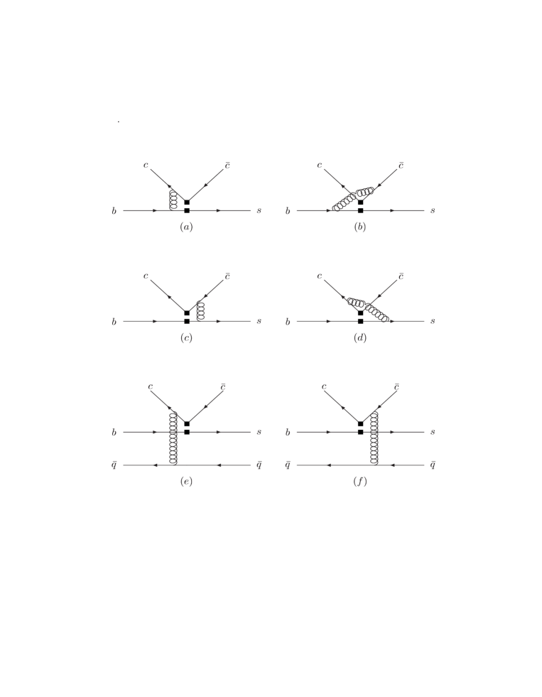
Figure 1: Feynman diagrams for nonfactorizable corrections to $\overline{B}\rightarrow\eta_{c}K$ decay.

As we can see easily in Eq. (6), this amplitude is unphysical because the Wilson coefficients depend on the renormalization scale $\mu$ while the decay constant and the form factors are independent of $\mu$. This is the well known problem with the naive factorization. However, if we include the order $\alpha_{s}$ corrections, it turns out that the $\mu$ dependence of the Wilson coefficients is cancelled and the overall amplitude is insensitive to the renormalization scale. Taking the nonfactorizable order $\alpha_{s}$ strong-interaction corrections in Fig. 1 into account, the full decay amplitude for $\overline{B}\rightarrow\eta_{c}K$ within the QCD factorization approach is written as

$$iM=if_{\eta_{c}}m_{B}^{2}F_{0}(m_{\eta_{c}}^{2})\frac{G_{F}}{\sqrt{2}}\Bigl{[}V_{cb}V_{cs}^{*}a_{2}-V_{tb}V_{ts}^{*}(a_{3}-a_{5})\Bigr{]},$$ (8)

where the coefficients $a_{i}$ ($i=2,3,5$) in the naive dimension regularization(NDR) scheme are given by

$$a_{2}=C_{2}+\frac{C_{1}}{N_{c}}+\frac{\alpha_{s}}{4\pi}\frac{C_{F}}{N_{c}}C_{1}\Bigl{(}-18+12\ln\frac{m_{b}}{\mu}+f_{I}+f_{II}\Bigr{)},$$

$$a_{3}=C_{3}+\frac{C_{4}}{N_{c}}+\frac{\alpha_{s}}{4\pi}\frac{C_{F}}{N_{c}}C_{4}\Bigl{(}-18+12\ln\frac{m_{b}}{\mu}+f_{I}+f_{II}\Bigr{)},$$ (9)

$$a_{5}=C_{5}+\frac{C_{6}}{N_{c}}-\frac{\alpha_{s}}{4\pi}\frac{C_{F}}{N_{c}}C_{6}\Bigl{(}-6+12\ln\frac{m_{b}}{\mu}+f_{I}+f_{II}\Bigr{)}.$$

The function $f_{I}$ in Eq.(9) is calculated from the four vertex corrections (a,b,c,d) in Fig. 1 and it reads

$$f_{I} = \int_{0}^{1}du\ \phi_{\eta_{c}}(u)\Bigl{[}\frac{3(1-2u)}{1-u}\ln[u]+3(\ln(1-z)-i\pi)-\frac{2z(1-u)}{1-zu}-\frac{2uz(\ln[1-z]-i\pi)}{1-(1-u)z}$$ (10)

$$- \frac{u^{2}z^{2}(\ln[1-z]-i\pi)}{(1-(1-u)z)^{2}}+uz^{2}\ln[uz]\bigl{(}\frac{u}{(1-(1-u)z)^{2}}-\frac{1-u}{(1-uz)^{2}}\bigr{)}$$

$$+ 2uz\ln[uz]\bigl{(}\frac{1}{1-(1-u)z}-\frac{1}{1-uz}\bigr{)}\Bigr{]},$$

where $z=m_{\eta_{c}}^{2}/m_{B}^{2}$, and we have already symmetrized the result with respect to $u\leftrightarrow 1-u$.

The function $f_{II}$ in Eq.(9) is calculated from the two spectator interaction diagrams (e,f) in Fig. 1 and it is given by

$$f_{II}=\frac{4\pi^{2}}{N_{c}}\frac{f_{K}f_{B}}{m_{B}^{2}F_{0}(m_{\eta_{c}}^{2})}\int_{0}^{1}d\xi\frac{\phi_{B}(\xi)}{\xi}\int_{0}^{1}du\frac{\phi_{\eta_{c}}(u)}{u}\int_{0}^{1}\frac{dx}{x}[\phi_{K}(x)+\frac{2\mu_{K}\phi_{K}^{p}(x)}{m_{b}(1-z)}],$$ (11)

where $\phi_{B}$ is the light-cone wave functions for the $B$ meson. The spectator contribution depends on the wave function $\phi_{B}$ through the integral

$$\int_{0}^{1}d\xi\frac{\phi_{B}(\xi)}{\xi}\equiv\frac{m_{B}}{\lambda_{B}}.$$ (12)

Since $\phi_{B}(\xi)$ is appreciable only for $\xi$ of order $\Lambda_{\mathrm{QCD}}/m_{B}$, $\lambda_{B}$ is of order $\Lambda_{\mathrm{QCD}}$. We will follow Ref. [3] to choose $\lambda_{B}\approx 300$ MeV in the numerical calculation.

	$C_{1}$	$C_{2}$	$C_{3}$	$C_{4}$	$C_{5}$	$C_{6}$
LO	1.144	-0.308	0.014	-0.030	0.009	-0.038
NDR	1.082	-0.185	0.014	-0.035	0.009	-0.041

Table 1: Leading-order(LO) and Next-to-leading-order(NLO) Wilson coefficients in NDR scheme(See Ref.[11]) with $\mu=4.4$ GeV and $\Lambda^{(5)}_{\overline{\rm MS}}=225$ MeV.

There is an integral in Eq. (11) arising from kaon twist-3 effects, which will give logarithmic divergence. Following Ref. [3], we treat the divergent integral as an unknown parameter and write

$$\int_{0}^{1}dx\frac{\phi_{K}^{p}(x)}{x}=\int_{0}^{1}\frac{dx}{x}=X_{H},$$ (13)

where $\phi_{K}^{p}(x)=1$ is used for the kaon twist-3 light-cone distribution amplitude. We will choose $X_{H}=\ln(m_{B}/\Lambda_{QCD})\approx 2.4$ as a rough estimate in our calculation.

For numerical analysis, we choose $F_{0}(m_{\eta_{c}}^{2})=0.41$[12] and use the following input parameters:

$$m_{b}=4.8\ \mbox{GeV},\ \ m_{B}=5.28\ \mbox{GeV},\ \ m_{\eta_{c}}=3.0\ \mbox{GeV},$$

$$f_{\eta_{c}}=350\ \mbox{MeV}\cite[cite]{[\@@bibref{}{constant}{}{}]},\ \ f_{B}=180\ \mbox{MeV},\ \ f_{K}=160\ \mbox{MeV}.$$ (14)

$\phi_{\eta_{c}}(u)$	$a_{2}$	$a_{3}$	$a_{5}$
$6u(1-u)$	0.1043-0.0684i	0.0045+0.0022i	-0.0035-0.0026i
$\delta(u-1/2)$	0.0792-0.0682i	0.0055+0.0022i	-0.0048-0.0026i

Table 2: The coefficients $a_{i}$ at $\mu=4.4$ GeV with different choices of $\phi_{\eta_{c}}(u)$.

The asymptotic form of the distribution amplitude $\phi_{\eta_{c}}(u)$ is given as $\phi_{\eta_{c}}(u)=6u(1-u)$. In the numerical analysis, we also consider the form $\phi_{\eta_{c}}(u)=\delta(u-1/2)$, which comes from the naive expectation of the distribution amplitude. Although there are uncertainties associated with the form of the wave function, we will see shortly that the calculated decay rates are not very sensitive to the choice of the distribution amplitude. The results of coefficients $a_{i}$ are listed in Table. 2.

With the help of these coefficients $a_{i}$, we calculated the decay branching ratios. For $\phi_{\eta_{c}}(u)=6u(1-u)$, ${\mathrm{Br}}(\overline{B}\rightarrow\eta_{c}K)=1.9\times 10^{-4}$. And for $\phi_{\eta_{c}}(u)=\delta(u-1/2)$, ${\mathrm{Br}}(\overline{B}\rightarrow\eta_{c}K)=1.4\times 10^{-4}$.

The measured branching ratios are

$$\mbox{CLEO Collaboration \cite[cite]{[\@@bibref{}{cleo}{}{}]}: }{\mathrm{Br}}(B^{0}\rightarrow\eta_{c}K^{0}) = (1.09^{+0.55}_{-0.42})\times 10^{-3},$$

$$\mbox{BaBar Collaboration \cite[cite]{[\@@bibref{}{babar}{}{}]}: }{\mathrm{Br}}(B^{0}\rightarrow\eta_{c}K^{0}) = (1.06\pm 0.28)\times 10^{-3},$$ (15)

$$\mbox{Belle Collaboration \cite[cite]{[\@@bibref{}{belle1}{}{}]}: }{\mathrm{Br}}(B^{0}\rightarrow\eta_{c}K^{0}) = (1.23\pm 0.23)\times 10^{-3},$$

which are about seven times larger than our theoretical results.

3 $B\rightarrow\eta_{c}^{\prime}K$ decay

The calculation of the branching ratio for $\overline{B}\rightarrow\eta_{c}^{\prime}K$ decay is similar to that for the $\eta_{c}$ given above. And we can also get a rough estimate for the decay rates ratio of $\eta_{c}^{\prime}$ to $\eta_{c}$ in the leading order:

$$\frac{{\mathrm{Br}}(B^{0}\rightarrow\eta_{c}^{\prime}K^{0})}{{\mathrm{Br}}(B^{0}\rightarrow\eta_{c}K^{0})}\approx\bigl{(}\frac{f_{\eta_{c}^{\prime}}}{f_{\eta_{c}}}\bigr{)}^{2}\cdot\bigl{[}\frac{F_{1}(m^{2}_{\eta_{c}^{\prime}})}{F_{1}(m^{2}_{\eta_{c}})}\bigr{]}^{2}\cdot\bigl{[}\frac{m^{2}_{B}-m^{2}_{\eta_{c}^{\prime}}}{m^{2}_{B}-m^{2}_{\eta_{c}}}\bigr{]}^{3}\approx 0.9\times\bigl{(}\frac{f_{\eta_{c}^{\prime}}}{f_{\eta_{c}}}\bigr{)}^{2}\approx 0.45,$$ (16)

where we have used $f_{\eta_{c}^{\prime}}/f_{\eta_{c}}\approx f_{\psi^{\prime}}/f_{J/\psi}$ with $f_{J/\psi}=400$ MeV, $f_{\psi^{\prime}}=280$ MeV, which are determeined from the observed leptonic decay widths [14]; and $F_{0}(p^{2})=(1-p^{2}/m_{B}^{2})F_{1}(p^{2})$ with $F_{1}(m^{2}_{\eta_{c}^{\prime}})=0.81,F_{1}(m^{2}_{\eta_{c}})=0.58$ [4, 12]. The ratio in Eq.(16) will roughly hold even when we include the $\mathcal{O}(\alpha_{\mathrm{s}})$ corrections, because the $\mathcal{O}(\alpha_{\mathrm{s}})$ corrections are small and the mass difference as well as the wave function difference between $\eta_{c}$ and $\eta_{c}^{\prime}$ will not change the values of $a_{i}$ in Eq.(9) greatly.

The Belle Collaboration has reported the observation of the $\eta_{c}^{\prime}$ in exclusive $B\rightarrow KK_{S}K^{-}\pi^{+}$ decays[10]:

$$\frac{{\mathrm{Br}}(B^{0}\rightarrow\eta_{c}^{\prime}K^{0}){\mathrm{Br}}(\eta_{c}^{\prime}\rightarrow K_{S}K^{-}\pi^{+})}{{\mathrm{Br}}(B^{0}\rightarrow\eta_{c}K^{0}){\mathrm{Br}}(\eta_{c}\rightarrow K_{S}K^{-}\pi^{+})}=0.38\pm 0.12\pm 0.05.$$ (17)

As was noted in Ref.[15], the hadronic decay branching fractions for $\eta_{c}$ and $\eta_{c}^{\prime}$ are expected to be roughly equal for the helicity non-suppressed decay channels. So we have ${\mathrm{Br}}(\eta_{c}^{\prime}\rightarrow K_{S}K^{-}\pi^{+})\approx{\mathrm{Br}}(\eta_{c}\rightarrow K_{S}K^{-}\pi^{+})$, and then from Eq.(17) we get

$$\frac{{\mathrm{Br}}(B^{0}\rightarrow\eta_{c}^{\prime}K^{0})}{{\mathrm{Br}}(B^{0}\rightarrow\eta_{c}K^{0})}\approx 0.4,$$ (18)

which is consistent with the ratio in Eq.(16). However, as was mentioned above, because the theoretical decay rate is about seven times smaller than the the experimental data for ${\mathrm{Br}}(B^{0}\rightarrow\eta_{c}K^{0})$, the theoretical branching fraction will also be about seven times smaller than the the experimental data for ${\mathrm{Br}}(B^{0}\rightarrow\eta_{c}^{\prime}K^{0})$.

4 Discussion

We have shown that for $B$ decays to $\eta_{c}$ and $\eta_{c}^{\prime}$ the theoretical branching fractions are all about seven times smaller than the experimental data. However, from Eq.(16) and Eq.(18), we see that the theoretical ratio of the decay rates of the two states is consistent with experimental data:

$$\frac{{\mathrm{Br}}(B^{0}\rightarrow\eta_{c}^{\prime}K^{0})}{{\mathrm{Br}}(B^{0}\rightarrow\eta_{c}K^{0})}_{Th.}\approx~{}\frac{{\mathrm{Br}}(B^{0}\rightarrow\eta_{c}^{\prime}K^{0})}{{\mathrm{Br}}(B^{0}\rightarrow\eta_{c}K^{0})}_{Ex.}.$$ (19)

It is also interesting to find that although the theoretical branching fractions of $B$ meson exclusive decays to $J/\psi$ and $\psi^{\prime}$ are both much smaller than the experimental data, the theoretical ratio of the decay rates of these two states is also roughly consistent with experimental data[14]:

$$\frac{{\mathrm{Br}}(B^{0}\rightarrow\psi^{\prime}K^{0})}{{\mathrm{Br}}(B^{0}\rightarrow J/\psi K^{0})}_{Th.}\approx\bigl{(}\frac{f_{\psi^{\prime}}}{f_{J/\psi}}\bigr{)}^{2}\cdot\bigl{[}\frac{F_{1}(m^{2}_{\psi^{\prime}})}{F_{1}(m^{2}_{J/\psi})}\bigr{]}^{2}\cdot\bigl{[}\frac{m^{2}_{B}-m^{2}_{\psi^{\prime}}}{m^{2}_{B}-m^{2}_{J/\psi}}\bigr{]}^{3}\approx 0.9\times\bigl{(}\frac{f_{\psi^{\prime}}}{f_{J/\psi}}\bigr{)}^{2}\approx 0.45,$$ (20)

$$\frac{{\mathrm{Br}}(B^{0}\rightarrow\psi^{\prime}K^{0})}{{\mathrm{Br}}(B^{0}\rightarrow J/\psi K^{0})}_{Ex.}\approx 0.6,$$ (21)

where $F_{1}(m^{2}_{\psi^{\prime}})=0.83$ and $F_{1}(m^{2}_{J/\psi})=0.61$ are used.

Another interesting observation is that the theoretical ratio of the branching fractions of $B$ meson exclusive decays to $\eta_{c}$ and $J/\psi$ is also roughly consistent with experimental data[7, 8, 9, 14]:

$$\frac{{\mathrm{Br}}(B^{0}\rightarrow\eta_{c}K^{0})}{{\mathrm{Br}}(B^{0}\rightarrow J/\psi K^{0})}_{Th.}\approx\bigl{(}\frac{f_{\eta_{c}}}{f_{J/\psi}}\bigr{)}^{2}\cdot\bigl{[}\frac{F_{1}(m^{2}_{\eta_{c}})}{F_{1}(m^{2}_{J/\psi})}\bigr{]}^{2}\cdot\bigl{[}\frac{m^{2}_{B}-m^{2}_{\eta_{c}}}{m^{2}_{B}-m^{2}_{J/\psi}}\bigr{]}^{3}\approx 1.0\times\bigl{(}\frac{f_{\eta_{c}}}{f_{J/\psi}}\bigr{)}^{2}\approx 0.75,$$ (22)

$$\frac{{\mathrm{Br}}(B^{0}\rightarrow\eta_{c}K^{0})}{{\mathrm{Br}}(B^{0}\rightarrow J/\psi K^{0})}_{Ex.}\approx 1.0.$$ (23)

Eq.(22) also approximately holds when $\mathcal{O}(\alpha_{\mathrm{s}})$ corrections are included.

So, the predicted relative rates of all S-wave charmonium states $J/\psi,\psi^{\prime},\eta_{c},\eta_{c}^{\prime}$ in the QCD factorization approach are roughly compatible with data. This has been shown explicitly above in the leading order approximation, and even holds when including $\mathcal{O}(\alpha_{\mathrm{s}})$ corrections with which the calculated decay rates for these four charmonium states are almost equally smaller than data by a factor of 7-10 though there are some theoretical uncertainties associated with form factors, decay constants, as well as the light-cone wave functions of mesons involved. This result is rather puzzling, and it might imply that the naive factorization for $B$ decays to the $S$-wave charmonia may still make sense but the overall normalization for the decay rates are questionable.

In summary, we have studied the exclusive decays of $B$ meson into pseudoscalar charmonium states $\eta_{c}$ and $\eta_{c}^{\prime}$ within the QCD factorization approach and find that the nonfactorizable corrections to naive factorization are infrared safe at leading-twist order. The spectator interactions arising from the kaon twist-3 effects are formally power-suppressed but chirally and logarithmically enhanced. The theoretical decay rates are too small to accommodate the experimental data. We already knew that for $B\rightarrow J/\psi K$ decay, there are also logarithmic divergences arising from spectator interactions due to kaon twist-3 effects and the calculated rates are also smaller than data by a factor of 8-10[4, 5]. Moreover, in our previous paper[6], we found that for $B\rightarrow\chi_{c1}K$ decay, the factorization breaks down due to logarithmic divergences arising from nonfactorizable spectator interactions even at twist-2 order, and the decay rates are also too small to accommodate the data, and that for $B\rightarrow\chi_{c0}K$ decay, there are infrared divergences arising from nonfactorizable vertex corrections as well as logarithmic divergences due to spectator interactions even at leading-twist order.

Considering the above problems encountered in describing $B\rightarrow\eta_{c}K(\eta_{c}^{\prime}K)$ as well as $B\rightarrow J/\psi K(\psi^{\prime}K)$ and $B\rightarrow\chi_{cJ}K(J=0,1)$ decays, we would like to restate our conclusion that in general the QCD factorization method with its present version can not be safely applied to exclusive decays of $B$ meson into charmonia, and that new ingredients or mechanisms should be introduced to describe exclusive decays of $B$ meson to charmonium states.

References

• [1] M. Beneke, G. Buchalla, M. Neubert and C.T. Sachrajda, Nucl. Phys. B 591 (2000)313.
• [2] M. Beneke, G. Buchalla, M. Neubert and C.T. Sachrajda, Phys. Rev. Lett. 83 (1999)1914.
• [3] M. Beneke, G. Buchalla, M. Neubert and C.T. Sachrajda, Nucl. Phys. B 606 (2001)245.
• [4] J. Chay and C. Kim, hep-ph/0009244.
• [5] H.Y. Cheng and K.C. Yang, Phys. Rev. D 63 (2001)074011.
• [6] Z. Song and K.T. Chao, hep-ph/0206253.
• [7] K.W. Edwards et al. (CLEO Collaboration), Phys. Rev. Lett. 86 (2001)30.
• [8] B. Aubert et al. (BaBar Collaboration), hep-ex/0203040.
• [9] F. Fang et al. (Belle Collaboration), hep-ex/0208047.
• [10] S.-K. Choi et al. (Belle Collaboration), Phys. Rev. Lett. 89 (2002)102001, Erratum-ibid.89 (2002)129901.
• [11] G. Buchalla, A.J. Buras and M.E. Lautenbacher, Rev. Mod. Phys. 68 (1996)1125.
• [12] P. Ball, JHEP 9809 (1998)005.
• [13] N. G. Deshpande, J. Trampetic, Phys. Lett. B 339 (1994)270.
• [14] D.E. Groom et al. (Particle Data Group), Eur. Phys. J. C 15 (2000)1.
• [15] K.T. Chao, Y.F. Gu and S.F. Tuan, Commun. Theor. Phys. 25 (1996)471.
• [16] Y.F. Gu, Phys. Lett. B 538 (2002)6.
• [17] M. Gourdin, Y.Y. Keum and X.Y. Pham, Phys. Rev. D 52 (1995)1597.
• [18] M. Gourdin, Y.Y. Keum and X.Y. Pham, Phys. Rev. D 51 (1995)3510.