HD-THEP-02-34
hep-ph/0209229
Triple gauge couplings
in polarised and their
measurement using optimal observables
M. Diehl111email: mdiehl@physik.rwth-aachen.de
Institut für Theoretische Physik E, RWTH Aachen, 52056 Aachen, Germany
O. Nachtmann222email: O.Nachtmann@thphys.uni-heidelberg.de and F. Nagel333email: F.Nagel@thphys.uni-heidelberg.de
Institut für Theoretische Physik, Philosophenweg 16, 69120 Heidelberg, Germany
Abstract
The sensitivity of optimal integrated
observables to electroweak triple gauge couplings is investigated for
the process fermions at future linear
colliders. By a suitable reparameterisation of the couplings we
achieve that all 28 coupling parameters have uncorrelated statistical
errors and are naturally normalised for this process. Discrete
symmetry properties simplify the analysis and allow checks on the
stability of numerical results. We investigate the sensitivity to the
couplings of the normalised event distribution and the additional
constraints that can be obtained from the total rate. Particular
emphasis is put on the gain in sensitivity one can achieve with
longitudinal beam polarisation. We also point out questions that may
best be settled with transversely polarised beams. In particular we
find that with purely longitudinal polarisation one linear combination
of coupling parameters is hardly measurable by means of the normalised
event distribution.
1 Introduction
The Standard Model (SM) of electroweak interactions has been thoroughly investigated both theoretically and experimentally and turned out to be very successful. After the discovery of the massive gauge bosons and , the direct measurement of the triple gauge couplings (TGCs), i.e. the couplings between two charged and one neutral gauge boson, has been an important issue at the TEVATRON and LEP as their values are determined by the non-Abelian electroweak gauge group. At colliders the production of pairs, single s, single photons and single s is suitable for that. In this paper we consider the process , where both the and the couplings can be measured at the scale given by the c.m. energy.
Deviations from the SM at the and vertices can be parameterised in a general framework. Allowing for complex couplings the most general vertex functions lead to altogether 28 real parameters [1]. All four LEP collaborations have investigated TGCs [2], the tightest constraints being of order for and , of order for and of order to for the real and imaginary parts of and/or violating couplings. All these values correspond to single parameter fits. Since only up to three-parameter fits have been performed, only a small subset of couplings has been considered at a time, thereby neglecting correlations between most of them. Moreover many couplings, notably the imaginary parts of and conserving couplings, have been excluded from the analyses.
At a future linear collider like TESLA [3] or CLIC [4], respectively covering a c.m. energy range from about 90 GeV to 800 GeV and from about 500 GeV to 5 TeV, one will be able to study these couplings with unprecedented accuracy. In this way one may begin to be sensitive to different extensions of the SM, which predict deviations at the TGCs from the SM values, typically through the effects of new particles and couplings in radiative corrections. Some examples, where effects of order may occur, are supersymmetric models [5, 6], models containing several Higgs doublets [7, 8], vector leptons [9] or Majorana neutrinos [10] and the minimal 3-3-1 model [11]. For left-right symmetric models [12, 13, 8] and mirror models [13] the effects are predicted to be much smaller, whereas models containing composite bosons [14] or an additional gauge boson [15] may lead to larger effects.
Given the intricacies of a multi-dimensional parameter space, the full covariance matrix for the errors on the couplings should best be studied. The high statistics needed for this will for instance be available at TESLA, where the integrated luminosity is projected to be about 500 or more per year at 500 GeV which for unpolarised beams amounts to about 3.7 million produced pairs (without cuts). For a run at 800 GeV the luminosity is expected to be twice as high, leading to 3.9 million pairs. Moreover, polarised beams will be particularly useful to disentangle different couplings. In fact, certain directions in the parameter space of the couplings, the so called right handed couplings, are difficult to measure in pair production with unpolarised beams [16]. In this case their effects are masked by the large contribution from the neutrino exchange. With polarised beams the strength of the neutrino exchange contribution can in essence be varied freely.
In experimental analyses of TGCs and various other processes, optimal observables [17, 16] have shown to be a useful tool to extract physics parameters from the event distributions. These observables are constructed to have the smallest possible statistical errors. Due to this property they are also a convenient means to determine the theoretically achievable sensitivity in a given process. In addition, they take advantage of the discrete symmetries of the cross section.
The method proposed in [18] allows one to simultaneously diagonalise the covariance matrix of the observables and the part of the cross section which is quadratic in the couplings. In this way one obtains a set of coupling constants that are naturally normalised for the particular process and—in the limit of small anomalous couplings—can be measured without statistical correlations. This allows one to see for which directions in parameter space the sensitivity to the TGCs is high and for which it is not, which is hardly possible by looking at covariance matrices of large dimension without diagonalisation. Moreover, the total cross section acquires a particularly simple form and provides additional constraints.
The basic purpose of this work is to use this extended optimal observable method for a systematic investigation of the prospects to measure the full set of TGCs in pair production at linear collider energies, with special emphasis on initial-state polarisation. The usefulness of the method becomes particularly evident when considering imaginary parts of conserving TGCs. In this subspace of couplings we find one direction to which—in the linear approximation and for longitudinally polarised beams—there is no sensitivity in the process we consider. In [18] this was not taken into account and led to numerical instabilities. It is therefore essential to disentangle the measurable TGCs from the hardly measurable one. As a historical motivation one may think of the electromagnetic nucleon form factors and , where the choice of linear combinations and leads to a simplification of the Rosenbluth formula for the differential cross section of electron-nucleon scattering (see e.g. [19]). Since we deal with 28 couplings here, an appropriate choice of parameters is essential.
We restrict ourselves to the semileptonic decays of the pair, where one boson decays into a quark-antiquark pair and the other decays leptonically, but leave aside the decay into since these events have a completely different experimental signature. The selected channels have a branching ratio of altogether , which is six times larger than that of both s decaying into or . On the other hand, the channels where both s decay hadronically are difficult to reconstruct [20]. The semileptonic channels have only one ambiguity in the kinematical reconstruction if the charges of the two jets from the hadronically decaying are not tagged. Then one cannot associate the jets to the up- and down-type (anti)quark of the decay, and therefore has access only to the sum of the distributions corresponding to the two final states.
This work is organised as follows: In Sect. 2 we recall the helicity amplitudes and cross sections of the process using a spin density matrix formalism. In Sect. 3 the optimal-observable method is presented in the form as it is used in our numerical calculations. We explain our technique to implement the simultaneous diagonalisation in a numerically stable way. The role of discrete symmetries in the framework of optimal observables is described. Many of the symmetry relations are well known, notably the classification of the TGCs into four symmetry classes [1] and its applicability to the optimal-observable method [16, 18]. Other properties are used for a check on the numerics. In Sect. 4 the dependence of the sensitivity on longitudinal beam polarisation is illustrated by a simple model. In Sect. 5 we show analytically that one is insensitive to one of the imaginary conserving couplings in the case of longitudinal beam polarisation. However, this particular coupling becomes accessible with transverse beam polarisation. In Sect. 6 we present our numerical results, in Sect. 7 our conclusions.
2 Cross Section
First we briefly recall the differential cross section of the process
| (1) |
for arbitrary initial beam polarisations, where the final state fermions are leptons or quarks. Our notation for particle momenta and helicities is shown in Fig. 1. Our coordinate axes are chosen such that the momentum points in the positive -direction and the unit vector is given by .

In the c.m. frame and at a given c.m. energy , a pure initial state of longitudinally polarised and is uniquely specified by the and helicities:
| (2) |
Note that fermion helicity indices are normalised to 1 throughout this work. A mixed initial state of arbitrary polarisation is given by a spin density matrix
| (3) |
where denotes summation over , , and , and the matrix elements satisfy and . We define the cross section operator
| (4) |
by requiring the differential cross section for arbitrary to be
| (5) |
The matrix is given by
| (6) |
where we neglect the electron mass in the flux factor. Here is the transition operator, the final state and
| (7) |
the usual phase space measure for final states. Using the narrow-width approximation for the s the result is
| (8) | |||||
| (9) |
Here is the boson mass, its width and its velocity in the c.m. frame. The sum runs over , , and . Furthermore
| (10) |
is the differential production tensor for the pair and
| (11) |
are the tensors of the and decays in their respective c.m. frames. Note that in the narrow-width approximation the intermediate s are treated as on-shell. We define the helicity states which occur on the right hand side of (10) in the frame of Fig. 1, i.e. we choose the scattering plane as the --plane and define to be the polar angle between the and momenta. We choose a fixed direction transverse to the beams in the laboratory. By we denote the azimuthal angle between this fixed direction and the scattering plane (see Fig. 2(a)).
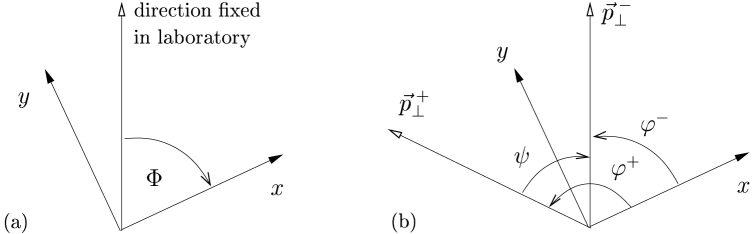
The respective frames for the decay tensors (11) are defined by a rotation by about the -axis of the frame in Fig. 1 (such that the momentum points in the positive -direction) and a subsequent rotation-free boost into the c.m. system of the corresponding . The spherical coordinates are those of the and momentum directions, respectively. In its rest frame, the quantum state of a boson is determined by its polarisation. For real s we take as basis the eigenstates of the spin operator with the three eigenvalues . For off-shell s a fourth, scalar polarisation occurs but is suppressed by in the decay amplitude.
Neglecting the electron mass we have in the SM
| (12) |
which we will use in the following (this point is further discussed in Sect. 3.3). At a linear collider the initial beams are uncorrelated so that their spin density matrix factorises, i.e.
| (13) |
where and are the two Hermitian and normalised spin density matrices of and respectively. We parameterise these matrices by
| (14) |
with
| (15) |
where , and the vector components of are the Pauli matrices. The degrees of transverse and of longitudinal polarisation obey the relations and . The components of in (15) refer to the frame of Fig. 1. Note that choosing the same reference frame for and while specifying each spinor in its respective helicity basis results in different forms of the density matrices in (14). The relative azimuthal angle between and is fixed by the experimental conditions, whereas the azimuthal angle of in the system of Fig. 1 depends on the final state (see Fig. 2(b)). For the case where we choose the transverse part of the vector as fixed direction in the laboratory. Then we have . Using (5) and (12) to (15), we obtain the differential cross section for arbitrary polarisation:
| (16) | |||||
In the absence of transverse polarisation, (16) is independent of due to rotational invariance.
In our analysis we evaluate the matrix elements in (10) at tree level in the SM, replacing the and vertices by their most general forms allowed by Lorentz invariance. The corresponding Feynman diagrams are shown in Fig. 3.
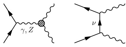
New physics may also lead to deviations from the SM values at the fermion-boson vertices [21]. For these vertices we however retain the SM expressions, following the rationale that at present they are confirmed experimentally to a much higher precision than the triple gauge couplings. We remark that there are scenarios of physics beyond the SM where such a treatment is not adequate, since the process can receive non-standard contributions that cannot be expressed in terms of anomalous fermion-boson or three-boson couplings (an example are box graph contributions in supersymmetric theories [5, 22]). Such effects can still be parameterised within a more general form factor ansatz [23]. If they are important, an analysis in terms of only TGCs will not give a correct picture of the underlying physics, but it will still correctly signal a deviation from the SM. We finally remark that radiative corrections in the SM itself can be included in the analysis procedure we develop here (see Sect. 3). The purpose of the present study is however to investigate the pattern of sensitivity to TGCs and its dependence on beam polarisation, and for this purpose it should be sufficient to take the SM prediction at tree level.
For the three-boson vertices we use the parameterisation (2.4) in Ref. [1], which we express in terms of the coupling parameters , , , , , and () by means of the transformation (2.5) in the same reference. In other words, we understand these parameters as form factors of the three-boson vertices, which depend on the boson virtualities and can take complex values, and not as coupling constants in an effective Lagrangian, which by definition are energy independent and real-valued.
For a given beam helicity the process (1) is not sensitive to all couplings, but only to the linear combinations , , etc. for left handed ( and , , etc. for right handed ( electrons, where
| (17) |
and similarly for the other couplings [1, 16]. Here denotes the positron charge, the weak mixing angle, and the ratio of the and photon propagators. The parameterisation (17) will in the following be called the L(eft)-R(ight)-basis.
The expressions of the amplitudes can be found in [1]. For convenience of the reader we rewrite the production part in terms of the LR-basis. The matrix element of (10) is given by
| (18) |
where , , , and . The definition of the -functions and our spinor conventions, as well as the SM matrix elements for the decays in (11) are listed in the Appendix. The production amplitude consists of two terms given by
| (19) | |||||
| (20) |
The expressions for (which contains the left handed couplings for and the right handed ones for ) and for and are listed in Table 1. Since the vector bosons carry spin 1, the TGCs do not contribute to the helicity combinations and . For the other helicity amplitudes, the largest power of in the coefficients coincides with the number of longitudinal s. An exception are the couplings and , which correspond to dimension-six operators in the effective Lagrangian (cf. [1]) and occur with an additional factor of . Note that the largest kinematical factors in behave like at high energies, in contrast to the basis of form factors used in Table 4 of [1], where huge factors of appear. In the SM at tree level one has
| (21) |
and all other couplings equal to zero. For the anomalous parts of the couplings we write and as usual.
A detailed discussion of the differential cross section is given in [1]. Here we only point out some salient features of the high-energy limit. In Fig. 4 we show the total cross section for unpolarised beams as a function of . It rises rapidly from threshold up to a maximum of about 20 pb at 200 GeV, and in the SM decreases for higher c.m. energies. In the SM each -coupling is equal to the corresponding photon coupling. Since the L-couplings are then of order 1 and the R-couplings of order . For this leads to a high energy behaviour of at most . For we have in the SM, and the coefficients and only differ by a factor according to Table 1. As they occur with different sign in (19) and (20) this again results in a high-energy behaviour , except for very forward momentum where there is an enhancement by the propagator factor . Altogether, these gauge cancellations preserve the unitarity of the SM. We also plot in Fig. 4 the total cross section for one anomalous coupling differing from zero. At high energies each coupling mainly contributes via the helicity amplitude where it occurs with the highest power of , i.e. either linearly or quadratically according to Table 1. At sufficiently high energy, the square of an anomalous term dominates over its interference term with the SM amplitude. In the limit the couplings , , and enter with a factor , whereas , , enter with a factor , which explains their different behaviour in Fig. 4. Some couplings have equal coefficients in this limit, which leads to a degeneracy of the curves. We also remark that even if more than one anomalous coupling differs from zero, anomalous amplitudes belonging to couplings of different or eigenvalue do not interfere in the total cross section with unpolarised beams (cf. Sect. 3.3).

3 Optimal Observables
In this section we discuss how the method of optimal integrated observables is applied to our case. In an experiment one measures the differential cross section
| (22) |
where denotes the set of all measured phase space variables. We distinguish between the information from the total cross section and from the normalised distribution of the events. We first investigate how well TGCs can be extracted from the latter, and then use to get constraints on those directions in the space of couplings to which the normalised distribution is not sensitive.
Since is a polynomial of second order in the anomalous couplings (defined as the couplings minus their tree-level values in the SM) one can write
| (23) |
Here is the tree-level cross section in the SM, and each is the real or imaginary part of an anomalous TGC. Thus there are 28 real parameters altogether. In the remainder of this section and each run from 1 to 28.
One way to extract the coupling constants from the measured distribution (23) is to look for a suitable set of observables whose expectation values
| (24) |
are sensitive to the dependence of on the couplings . Given the present experimental constraints, we expect these variations to be small. Thus we expand the expectation values to first order in :
| (25) |
with
| (26) | |||||
| (27) | |||||
| (28) |
Here is the expectation value for zero anomalous couplings, whereas gives the sensitivity of to . Solving (25) for the set of the we get estimators for the anomalous couplings, whose covariance matrix is given by
| (29) |
where we use matrix notation. Here is the number of events, and
| (30) |
is the covariance matrix of the observables, which we have Taylor expanded around its value in the SM. As observables we choose
| (31) |
From (27) and (30) one obtains for this specific choice
| (32) |
and therefore
| (33) |
The observables (31) are “optimal” in the sense that for the errors (33) on the couplings are as small as they can be for a given probability distribution.444For details on this so called Rao-Cramér-Fréchet bound see e.g. [24, 25]. Apart from being useful for actual experimental analyses, the observables (31) thus provide insight into the sensitivity that is at best attainable by any method, given a certain process and specified experimental conditions. In the case of one parameter this type of observable was first proposed in [17], the generalisation to several parameters was made in [16]. Moreover, it has been shown that optimal observables are unique up to a linear reparameterisation [18]. We further note that phase space cuts, as well as detector efficiency and acceptance have no influence on the observables being “optimal” in the above sense, since their effects drop out in the ratio (31). This is not the case for detector resolution effects, but the observables (31) are still close to optimal if such effects do not significantly distort the differential distributions and (or tend to cancel in their ratio). To the extent that they are taken into account in the data analysis, none of these experimental effects will bias the estimators.
In the present work we use the method of optimal observables in the linear approximation valid for small anomalous couplings. But we emphasise that the method has been extended to the fully non-linear case where one makes no a priori assumptions on the size of anomalous couplings in [18]. Such a non-linear analysis for real data was presented in [20] and turned out to be very convenient and highly efficient.
Given the projected accuracy at linear colliders, it will in general be necessary to take into account radiative corrections to the process within the SM, which have been worked out in detail in the literature [26]. One possibility to include them in searches for non-standard TGCs would be to “deconvolute” these corrections. For this write the one-loop corrected differential cross section in the SM as
| (34) |
where is the tree-level expression, and the integral kernel can e.g. be obtained from an event generator by generating events according to both and . Approximating the true physical cross section as
| (35) |
with given as in (23), one could invert this convolution bin by bin, and then extract the couplings from the deconvoluted Born level cross section as described before. The error made in (35) is that the SM radiative corrections encoded in do of course not apply to the anomalous part of the cross section, but this error is of order times the weak coupling constant . Should effects beyond the SM be found in such an analysis, one would in a second step have to consider more sophisticated methods to quantitatively disentangle them from SM radiative corrections.
3.1 Simultaneous Diagonalisation
Although discrete symmetry properties (see Sect. 3.3) reduce the 2828 matrices , , etc. to blocks of 88 and 66 matrices, these blocks still contain many non-negligible off-diagonal entries. To make explicit how sensitive the process is to each direction in the space of couplings and to identify the role of polarisation we need to know directions and lengths of the principal axes of the error ellipsoid defined by (29), i.e. we have to know the eigenvalues and eigenvectors of . Using optimal observables, to leading order in the , the three matrices , and are automatically diagonalised simultaneously due to (32) and (33). This means that after such a transformation each observable is sensitive to exactly one coupling, and the observables as well as the estimators of the couplings are statistically independent. Since is symmetric the diagonalisation could be achieved by an orthogonal transformation. Following the proposal of [18] we take however a different choice and transform simultaneously into diagonal form and the normalised second-order part of the total cross section into the unit matrix:
| (36) |
This can always be done since is symmetric and positive definite. We therefore arrive at the following prescription for the transformation of the couplings (using vector and matrix notation):
| (37) | |||||
| (38) | |||||
| (39) |
where are the one-sigma errors on the new couplings. This transformation exists and is unique up to permutations and a sign ambiguity for each . Note that the matrix is in general not orthogonal. From (23), (31) and (37) the transformation of all other quantities follows as
| (40) |
The meaning of (39) is that all quadratic terms contribute to the total cross section with equal strength:
| (41) |
where . Thus the anomalous couplings do not mix in and are “naturally” normalised for the process which we consider. This is not true in the conventional basis, where changing different anomalous couplings by the same amount has completely different effects on the total cross section (see Fig. 4 in Sect. 2).
Moreover, the particularly simple form (41) of easily allows one to use the information from the total rate: it constrains the couplings to lie between two hyperspheres in the space of the , whose difference in radius depends on the measurement error on . Making in addition use of the sign ambiguity in (37), one can for all choose the sign of such that . This choice is however not relevant for the analysis.
We finally note that the presented method of simultaneous diagonalisation is quite similar to the way one analyses the normal modes of a multi-dimensional harmonic oscillator in classical mechanics [29]. There the harmonic potential (corresponding to ) is diagonalised with respect to the scalar product defined by the kinetic energy (corresponding to ).
3.2 Numerical Realisation
We now give some details of how the simultaneous diagonalisation can be carried out numerically. Although the procedure finally aims at the disentanglement of the couplings as achieved in (38), the numerical computation of or from (29) needs the inverse of the matrix or and might therefore be unstable, because before the diagonalisation one cannot single out those directions in parameter space where the errors are large. However, as and are simultaneously diagonal for our observables, we can according to (32) equally well compute the diagonal entries of
| (42) |
and extract the errors on the couplings using (33):
| (43) |
Hence, using the shorthand notation and , we have to solve the equations
| (44) |
for the entries of and the diagonal elements of . Since the multiplication of by a constant changes neither the observables (31) nor nor , the matrices and only depend on the normalised distribution of the events but not on the total rate . The latter enters the errors on the transformed couplings only through the statistical factor in (43). From (44) it follows that
| (45) |
This is a generalised eigenvalue problem, with the being the generalised eigenvalues and the columns of being the generalised eigenvectors. The pair is called the “eigensystem” of (44). A standard method for solving (45) is to first perform a Cholesky decomposition [27, 28]
| (46) |
where is a lower triangular matrix, i.e. for . Algorithms for the computation of can be found in the same references. Then (45) is equivalent to
| (47) |
where
| (48) | |||||
| (49) |
Equation (47) denotes a (usual) eigenvalue problem for the matrix , whose eigenvalues are the same as the original ones and whose eigenvectors are the columns of . Since is symmetric, (47) can be solved and the eigenvectors are orthogonal with respect to the standard scalar product (assuming non-degeneracy of the eigenvalues). Requiring the eigenvectors to be normalised to 1, we have conditions
| (50) |
which together with the equations (47) are equivalent to (44). The generalised eigenvectors are obtained by solving (49) for . The procedure has to be followed for each initial state polarisation and c.m. energy separately, leading in general to different eigenvalues and transformation matrices; the dependence of those quantities on polarisation is investigated in Sect. 4. In each case we use the procedure iteratively, i.e. once is obtained, we compute and for the transformed observables and couplings, and then diagonalise these—already approximately diagonal—matrices again. We found this to be essential to assure the numerical stability of the results. A stable value was reached in most cases by the second evaluation and at the latest by the fourth. In all cases at least five evaluation steps were carried out. The numbers presented in Sect. 6 were obtained by averaging over the results of several subsequent steps where the stable value had already been reached.
We note that for situations where and have the same block diagonal structure, the diagonalisation can of course be carried out for each block separately. This is relevant in the presence of discrete symmetries.
3.3 Discrete Symmetries
Let us now discuss the special role of the combined symmetry operations and in the context of our reaction [1, 16, 18]. Here denotes charge conjugation, parity reversal, and “naïve time reversal”, i.e. the reversal of all particle momenta and spins without the interchange of initial and final state. Under the condition that the initial state, as well as phase space cuts and detector acceptance are invariant under a transformation, a odd observable gets a nonzero expectation value only if is violated in the interaction. Similarly, if the initial state, phase space cuts and acceptance are invariant under followed by a rotation by 180∘ around an axis perpendicular to the beam momenta, a nonzero expectation value of a odd observable implies the interference between absorptive and nonabsorptive amplitudes in the cross section. In terms of the three-boson couplings one finds that to the expectation values of even (odd) observables only involve the conserving (violating) couplings , , , (, , ). Similarly, even (odd) observables are to first order only sensitive to the real (imaginary) parts of the coupling parameters. The coefficient matrix is thus block diagonal in the following groups of observables:
(a): and even,
(b): even and odd,
(c): odd and even,
(d): and odd.
One further finds that the first-order terms in the integrated cross section can only be non-zero for couplings of class (a).
The above requirements on the initial state are nontrivial in the case of polarised beams. Since charge conjugation exchanges and , a invariant spin density matrix requires , in particular and . Under the same conditions the density matrix is also invariant under times a rotation by 180∘ around . Let us investigate the situation where these requirements are not satisfied. From Fig. 5 we see that the states where the beam helicities are aligned are eigenstates. But the antialigned () states are interchanged under and therefore are not eigenstates. On the other hand, the amplitudes for these helicity combinations are proportional to the electron mass in the SM (supplemented by the most general TGCs). They are thus generically suppressed by compared with the amplitudes for aligned beam helicities ().555To be precise, one must exclude final states , where nonresonant graphs contribute in which the initial and do not annihilate. With transverse beam polarisation, the two types of amplitudes can interfere, giving small effects in the cross section. With purely longitudinally polarised beams they do not interfere, so that effects due to the combinations of are of order and thus beyond experimental accuracy. We remark that the same holds e.g. in the minimal supersymmetric extension of the SM, where left- and right handed leptons as well as their superpartners only mix with a strength proportional to the lepton mass. To investigate what can happen in more generic models is beyond the scope of this work.

For general beam polarisation, a nonzero mean value of a odd observable can be generated by genuine violation in the reaction, or by the odd part of the spin density matrix in the initial state. According to the above estimate, the latter would require nonstandard physics to be experimentally visible, especially for longitudinal beam polarisation, and thus be interesting in its own right. Similarly, a nonzero result for a odd observable can originate from absorptive parts in the process, or from effects of the amplitudes with zero total helicity of the initial beams. If any such effects were observed, one could in a next step investigate their dynamical origin, using their different dependences on the beam polarisation. One possibility is to use that in the absence of amplitudes the cross section depends on transverse beam polarisation only via the product , as seen in (16). If , the cross section is then independent of and , whereas the interference between and amplitudes leads to terms with and to the cross section, which can experimentally be identified via their angular dependence on . A possibility to search for the presence of amplitudes with only longitudinal beam polarisation will be discussed at the end of Sect. 4.
Returning to purely longitudinal beam polarisation and the assumption that amplitudes are negligible, we remark that constraints similar to the ones discussed above cannot be derived for and separately, since neutrino exchange maximally violates both symmetries. One can however classify the TGCs according to their and behaviour as shown in Table 2. As can be seen from the amplitudes in Sect. 2, terms of distinct or do not mix in the quadratic part of the total cross section
| (51) |
provided that phase space cuts are separately invariant under and . Under the same conditions the linear terms in the integrated cross section for the couplings , , and vanish. This is due to the absence of the neutrino exchange graph for right handed electrons and the fact that those couplings differ in their or eigenvalues from the TGCs in the SM. Finally, real and imaginary parts of couplings do not mix in .
In the LR-basis, has an additional block diagonality, with two separate blocks for the R- and the L-couplings, which cannot mix in the total cross section. Any block diagonality of means that already before the simultaneous diagonalisation (40) the subspaces corresponding to these blocks are perpendicular to each other with respect to the scalar product . As a consequence, two row vectors of or two column vectors of which correspond to different blocks are perpendicular with respect to the standard scalar product. In the case of this follows from the first equation of (44) by solving for , and in the case of by solving for . The comparison of the matrix products and with this expected orthogonality thus provides a good way to test the numerical results for and . Note however that the transformation described in Sect. 3.1 cannot be carried out on smaller blocks than those given by the four classes (a) to (d) because the left handed couplings mix with the right handed ones in , and .
4 Polarisation
In this section we explore how the sensitivity of our process to anomalous TGCs depends on the longitudinal polarisation of the initial beams. To this end we will introduce an appropriate polarisation parameter and analyse how the eigensystem determined by (44) depends on it. This may be seen as a preparation for interpreting the numerical results in Sect. 6, which will be given in terms of the same parameter.
To start with, we introduce a convenient notation to make explicit the polarisation dependence of the matrices and , which have to be diagonalised simultaneously according to (44). In the following we restrict ourselves to the case of longitudinally polarised beams. Since in the limit only two beam helicity combinations contribute to the amplitudes, we can use (16) to write the differential cross section in terms of the cross sections and for purely left and right handed beams (and opposite helicities),
| (52) |
where
| (53) | |||||
| (54) |
and . Since we only deal with longitudinal polarisation in this section we drop the subscript ’’ in the polarisation parameters. Note that . Integrating over one obtains the total cross section as
| (55) |
In the LR-basis we have
| (56) | |||||
| (57) |
We denote again the real or imaginary parts of the anomalous TGCs by , but in contrast to (23) we now explicitly write an index , so that and only run from 1 to 14. Using vector and matrix notation we can rewrite the total cross section as
| (58) |
where
| (63) | |||||
| (66) |
with vectors and and the matrix . In the LR-basis and for longitudinal polarisation we thus obtain the following expression for the covariance matrix (30):
| (67) |
with . Let us now investigate in detail how the eigensystem of and depends on and . It is useful to express and by new variables and (to be specified below), so that , and hence also their eigensystem only depend on . For this purpose we introduce and through
| (68) |
for some well-behaved rescaling function , and define the “-normalised” quantities
| (69) | |||||
| (70) |
We then have from (66) and (67):
| (73) | |||||
| (74) |
where we have made the dependence on explicit. Note that the left hand sides of (73) and (74) depend on but not on , since and do not change when is multiplied by a constant. For the matrix in (46) we get
| (75) |
where is the Cholesky decomposition of the independent submatrix of . Then the result for the transformation (37) is
| (78) | |||||
The factors and in the rightmost matrix determine the mutual normalisation of the blocks of left and right handed couplings. They let become singular in the limits or . This is not surprising because with beams of purely longitudinal polarisation one is sensitive to only half of the couplings. The coefficient in (78) leads to an overall normalisation which strongly depends on the polarisation. At GeV we have for instance
| (79) |
whereas at TeV the ratio is about 30. From (50) we see that the matrix is orthogonal for any . In the case of pure polarisation it is block diagonal in the left and right handed couplings. This is however not the case for general (longitudinal) polarisation since the diagonalisation cannot be reduced to smaller blocks than those given by the four discrete symmetry classes introduced in Sect. 3.3.
We now specify the transformation (68) by choosing
| (80) |
and defining a polarisation parameter
| (81) |
with values . We then have
| (82) |
In terms of the individual beam polarisations and the parameters and are given as
| (83) | |||||
| (84) |
The reason for this particular choice is as follows. For electron polarisation and positron polarisation one simply has . For general polarisations is between and , and the differential cross section for equals the one for up to a constant. The eigenvalues (cf. (42)) are hence the same for and for .
To develop some intuition of how the generalised eigenvalues of (73) and (74) depend on , we consider the case of only one left and one right handed coupling. Moreover, we neglect the second term in (74), which appears only in symmetry class (a). The matrix in (66) then reduces to a single number , the vector has only one component , and the 22 matrices which have to be diagonalised according to (44) can be written as
| (87) | |||||
| (94) |
where
| (95) |
As in (48) we construct a symmetric matrix
| (96) |
whose usual eigenvalues are equal to the generalised eigenvalues of , i.e. to the diagonal entries of the transformed matrix in (44). They are given by
| (97) |
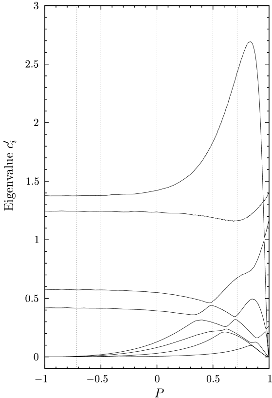
We approximate the matrix entries (95) by
| (98) |
with constants , which should take into account their dependence sufficiently well for a qualitative model. In Fig. 7 we plot the eigenvalues in arbitrary units for , and , with the last number taken from (79). The ratios in our choice of parameters are motivated by the power of in (95), which corresponds to the power of the neutrino exchange amplitude in the cross section. One can show analytically that the slopes of the curves for tend to zero for . For this cannot be seen in the plot, since for large (i.e. ) the eigenvalues change rapidly as the beam becomes purely right-handed. To see the horizontal tangent we plot a second example in Fig. 7 with a more moderate value of . Notice that for nonzero the two curves for and do not touch. If or is zero the matrix in (87) and hence in (96) is singular, which leads to a zero eigenvalue at .


As in Sect. 3.2 let
| (99) |
be the matrix whose columns are the normalised eigenvectors of . We can see from Figs. 7 and 7 that for the vector with large eigenvalue has only an upper component (corresponding to ), whereas the vector with zero eigenvalue has only a lower component (corresponding to ). For the situation is reversed. This reflects the fact that one is only sensitive to the left handed couplings for and to the right handed ones for . We finally plot the elements of the transformation matrix in (78) using the notation
| (100) |
Writing the transformed couplings as
| (101) |
we can see that for the right handed contributions to both and vanish, whereas for the same happens to the left handed ones. This behaviour of has to be taken into account when carrying out the simultaneous diagonalisation for high degrees of longitudinal polarisation, because it leads to a singularity of its inverse in the limit .
We have seen that under the condition that only beam helicity combinations with contribute to the cross section, the expectation values of normalised observables only depend on the polarisation parameter . Such a statement no longer holds if beams with helicities coupled to contribute as well. This provides a possibility to disentangle effects from genuine violation or absorptive parts from those due to nonzero amplitudes. In particular, the odd part of the spin density matrix for longitudinally polarised beams is proportional to and will give different contributions to normalised observables if is varied for fixed .
5 Hardly Measurable Couplings
The particular form of the SM amplitudes for the process has consequences on its sensitivity to the couplings in the conserving sector, which we shall now discuss. To this end we write the TGC part of the transition operator as
| (102) |
where for simplicity of notation we label the respective couplings , , , , , , by an index . Here are the SM couplings in the LR-basis and are the complex anomalous couplings (which we write in uppercase to distinguish them from the real-valued parameters ). The nonzero SM couplings are (see (21), (17))
| (103) |
We first consider longitudinal polarisation where the differential cross section (cf. 22)) is given by (52). For there is no neutrino exchange contribution, so that we have from (6), (54) and (102)
| (104) | |||||
Consider now the following direction in the space of right handed anomalous couplings:
| (105) |
where we assume and use the vector notation
| (106) |
With (105) the second line of (104) equals
| (107) |
In the space of the imaginary parts of right handed couplings there is hence a direction in which the differential cross section for unpolarised or longitudinally polarised beams has no linear term in , but is only sensitive to order . This direction is determined by the real SM couplings as given by (103). Therefore, one of the functions and the corresponding observable in (40) are identically zero, and contains one (usual as well as generalised) eigenvalue in symmetry class (b) that is zero for all values of . This is confirmed by our numerical results shown in Figs. 10, 14 and 18. In the tables in Sect. 6 the eigenvalues of symmetry class (b), , are given in decreasing order. Using this notation we have
| (108) |
From the total rate one can derive constraints on this coupling as explained in Sect. 3.
Now consider
| (109) |
which merely “stretches” the right handed SM couplings by a factor . Then the last line of (104) becomes
| (110) |
In the case of purely right handed electrons or left handed positrons, i.e. for , we have from (52), so that the anomalous coupling (109) only increases the total rate but does not affect the normalised distribution . This holds both to order and to order . Symmetry class (a) therefore contains a fifth zero eigenvalue for , in addition to the four zero eigenvalues from the left handed couplings Re, Re, Re and Re, which cannot be measured for . This is again confirmed by our numerical results (cf. Figs. 9, 13, 17). For , however, also contributes to . Since the functions are not identical for and , the enhancement of due to (110) will not just change by an overall factor, but also modify the normalised distribution . The latter is sensitive to the anomalous TGC in (109) in the linear approximation, since (110) contains a term linear in . In contrast to symmetry (b), there is thus no eigenvalue which is identical to zero for all values of . Note that contains interference terms of the left handed anomalous amplitudes and the SM neutrino exchange, so that the arguments above do not apply to the subspace of the left handed couplings. Also for the symmetries (c) and (d) there is no similar argument because violating TGCs are absent in the SM at tree level.
The direction (105) in coupling space becomes measurable in the linear approximation with beams of transverse polarisation. In fact, abbreviating
| (111) |
where is the transition operator in the SM at tree level and is defined in (102), we can write the part of the differential cross section (16) that is linear in the anomalous TGCs as
where of course implies and implies . As in Sect. 2 we denote the degrees longitudinal and transverse polarisation of the and beams by and , and as in Sect. 4 we abbreviate and . Note that depends on the azimuthal angle only via the explicit trigonometric functions in (5). One thus only has if the three lines of (5) vanish separately. The first line is however the same as what we had for purely longitudinal polarisation, so that it vanishes for generic polarisations only if condition (105) is fulfilled and . Then relation (5) becomes:
where for the equality we have used the fact that . Since contains the neutrino exchange graph, no longer vanishes. Transverse beam polarisation thus allows for the measurement of the anomalous coupling (105), which is hardly possible using only longitudinal polarisation.
Before presenting our numerical results for unpolarised and longitudinally polarised beams, we must explain how to take into account the zero eigenvector (105) of in the analysis. From (33) and (40) we obtain for the inverse covariance matrix of the couplings
| (114) |
where the are again 28 real parameters, viz. the real and imaginary parts of , , , , etc. We number the couplings in the order of their symmetry class (a) to (d), and within each symmetry class take the L-couplings first. We then have and . Note that always exists, even in our case where one parameter is unmeasurable. In this case is a singular matrix with a one-dimensional zero eigenspace coming from . Geometrically speaking, the error ellipsoid defined by is degenerate in such a way that the length of one principal axis is infinite. Instead of an ellipsoid we have a cylinder whose axis corresponds to the direction of the unmeasurable coupling and whose cross-section (orthogonal to the axis) is an ellipsoid giving the errors on the couplings in the orthogonal space. We know from (103) and (105) that the unmeasurable direction is given by with all other couplings being zero. Therefore the projection of the cylinder onto the --plane is a band in the -direction, see Fig. 8(a).
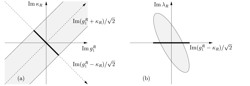
This shows that we cannot obtain any constraint on or unless one of them is known. We can however choose coordinate axes parallel and orthogonal to the band shown in Fig. 8(a). In other words, we perform a rotation by in the --plane,
| (115) |
where is the identity matrix except for the --block, which reads
| (116) |
The new couplings are the same as the , except for and , which replace and . The inverse covariance matrix of the new couplings is
| (117) |
All entries in the 14th row and in the 14th column of are equal to zero: there is no correlation between the unmeasurable -direction and the couplings with . These couplings are hence constrained by a 27-dimensional ellipsoid, which is drawn schematically in Fig. 8(b) for one further coupling, taken to be . This ellipsoid is determined by the “reduced” matrix obtained from by deleting the 14th row and the 14th column. Its inverse is the covariance matrix of and the other 26 measurable couplings. In particular, the width of the band in Fig. 8(a) gives the error on in the presence of all other 27 couplings , cf. Fig. 8(b). We finally mention that because of the discrete symmetries explained in Sect. 3.3, the matrix is block diagonal with one block for each symmetry class (a) to (d), so that the errors on the couplings of class (a), (c) and (d) are entirely unaffected by the previous discussion.
6 Numerical Results
In this section we present the results for the generalised eigenvalues of the covariance matrix and the corresponding errors on the transformed couplings. The covariance matrix for the couplings in any other parameterisation is then obtained by conventional error propagation. We discuss its most important properties in the LR-basis for and unpolarised beams in Sect. 6.1. In Sect. 6.2 we investigate the gain in sensitivity by longitudinal as well as additional polarisation. The results for higher c.m. energies are reported in Sect. 6.3. In Sect. 6.4 we finally give the constraints which can be obtained from the total rate according to (41). Numerical rounding errors on the results presented in this section are typically of order 1%.
We use and from [25], and the definition for the weak mixing angle. For the total event rate of the semileptonic channels with and summed over we use the values listed in Table 3. They correspond to an effective electromagnetic coupling constant and integrated luminosities of 500 , 1 and 3 at , 800 GeV and 3 TeV, respectively. We assume full kinematical reconstruction of the final state, except that the jet charges are not tagged. Due to this twofold ambiguity we cannot take the zeroth and first order parts of the differential cross section as the denominator and the numerator of the optimal observables , but use their respective sums over the two experimentally undistinguished final states (cf. [16]).
| polarisation | [GeV] | ||||
|---|---|---|---|---|---|
| 500 | 800 | 3000 | |||
| 3280 | 3410 | 1280 | |||
| 2050 | 2130 | 799 | |||
| 1140 | 1190 | 444 | |||
| 235 | 242 | 89.7 | |||
| 103 | 103 | 37 | |||
6.1 Unpolarised Beams at 500 GeV
We first consider the sensitivity at 500 GeV with unpolarised beams. In Tables 4–7 we list the standard-deviation for each coupling , which gives its error in the presence of all other couplings. Notice the difference of this to , which corresponds to the error on when all other couplings are assumed to be zero. We also give the correlation matrix
| (118) |
of the couplings for each symmetry class (a) to (d). In the case of symmetry (b) we use the reduced matrix introduced in Sect. 5. Since is symmetric we only list its upper triangular part.
The values of range from about to within each symmetry class. The smallest are those for , and since at high energies the corresponding terms in the helicity amplitudes contain a factor (cf. Table 1). In all cases the errors on the R-couplings are larger than those on the respective L-couplings, viz. by a factor 1.5 to 3.4 for Im, Re and Re, and by a factor between 4 and 7 for the other couplings. This is because (for unpolarised or longitudinally polarised beams) the -exchange interferes with the amplitudes containing the , but not with those containing the . In general, the sensitivity to the real part of a specific coupling is roughly of the same size as the sensitivity to its imaginary part, the errors on the latter being rather larger for conserving couplings and smaller for the violating ones. To get an accurate picture of the sensitivities, correlations have to be taken into account. Looking at the 22 blocks corresponding to and for a given index , i.e. at the diagonal entries of the right upper block in the correlation matrices, we see that the absolute values of the correlations are smaller than about 0.2, except for Re, Im and Im, where they are still smaller than 0.6. The corresponding correlations would be substantial in the basis of the - and -form factors, which is hence not a very suitable parameterisation for the present reaction, compared with the LR-basis (cf. [16]). Considering the matrix blocks of correlations among different L-couplings or among different R-couplings, we find that about half of them have an absolute value larger than 0.4. Note that there are correlations of order 0.5 between couplings with different or eigenvalues.
By simultaneous diagonalisation (see Sect. 3.1) we determine the generalised eigenvalues and corresponding errors given in Tables 8 and 9. For symmetry class (b) we give the transformation matrix and its inverse in Tables 10 and 11.666The matrices for symmetry classes (a), (c) and (d) can be obtained from the authors. Further numerical results for unpolarised and longitudinally polarised beams at various c.m. energies are given in [30]. In our numerical calculation we find the smallest eigenvalue in symmetry class (b) to be . We can however use the result of our analytical considerations in Sect. 5 and set to zero. The same holds for the last column of except for its Im- and Im-components, which determine the corresponding “blind” direction in the LR-basis. As explained in Sect. 3.3 the odd coupling does not mix with the other couplings in , and the same is true for the left and right handed couplings. From this block structure of and the relation it follows that in the last row of we can set all entries to zero, except for the Im-, Im- and Im-components. Numerically we find that the absolute values of those matrix entries which we set to zero are smaller than for and smaller than for . We remark that we have computed the matrix by inverting using singular value decomposition [28]. As mentioned at the end of Sect. 3.3 we have as a further check evaluated the products and .
6.2 Polarised Beams
At future -colliders longitudinal polarisation of both initial beams is envisaged [31, 32, 33]. An electron polarisation of and a positron polarisation of is considered to be achievable.
In Tables 12 and 13 we give the errors on the real couplings (in the presence of all couplings) for 500 GeV and various combinations of beam polarisations. For all couplings and all couplings we find roughly the following gain or loss in sensitivity using always the event rates of Table 3. Turning on polarisation of we gain a factor of 1.4 for and loose a factor of 6 for . If in addition we gain a factor of 1.8 for and loose a factor of 17 for compared to unpolarised beams. For we loose a factor of 2.6 for and gain a factor of 3.0 for . If furthermore we loose a factor of 5 for and gain a factor of 5.5 for compared to unpolarised beams. Especially for the right handed couplings the gain from having both beams polarised is thus appreciable.
The behaviour of the generalised eigenvalues as a function of the parameter introduced in Sect. 4 is shown in Figs. 9–20. Although the four largest eigenvalues are more or less constant for , the transformation matrix is not. This can be seen from Tables 14, 15 and 16. For the largest eigenvalue of symmetry (a) we find that the smaller is, the more the R-components are suppressed, i.e. the more one purely measures the . Going from to we become more and more sensitive to the . For the fourth lowest curve in Fig. 9, corresponding to , as well as for the smallest eigenvalue of symmetry (a) we find the opposite tendency. Note that in the case of electron or positron polarisation we can only be sensitive to at most half of the couplings. This is seen for symmetries (c) and (d) in Figs. 11, 12, 15, 16, 19 and 20: half of the curves go to zero at . For class (a) (cf. Figs. 9, 13 and 17) we find one additional eigenvalue going to zero at and for class (b) (cf. Figs. 10, 14 and 18) there is a zero eigenvalue for all , as explained in Sect. 5. Comparing with Fig. 7 we see that for symmetries (b) to (d) the shape of the curves is qualitatively well described by the simple model of Sect. 4. Although the lower and upper curves for do not intersect in our examples there, an intersection like in Fig. 11 is not excluded. In general, it is however not possible to associate a certain pair of couplings to a pair of curves in Figs. 9–20 for the full range of . This is particularly obvious from the eigenvalues of symmetry (c) at TeV (Fig. 19), where some curves alternately play the role of the lower-type and upper-type curves in the simplified model. Moreover, for symmetry class (a) the description of the shape of the eigenvalue curves is less obvious due to the second term in the brackets of (67).
6.3 Energy Dependence
The gain in sensitivity when going up from 500 GeV to 800 GeV—using always the event rates of Table 3—lies between 1.4 and 2.7 for all couplings except for Im, where it is 3.6. At 3 TeV we gain a factor of about 25 compared to 800 GeV for this coupling, and of 1.5 to 8 for all others. For symmetries (a) and (c) we give in Tables 17 and 18.
Note that this gain is not due to the the total rate, which actually decreases with energy (cf. Table 3). The largest gains are achieved for , and , which have a prefactor in the amplitude. We remark that both for real and imaginary parts the gains in sensitivity for an L-coupling and the corresponding R-coupling are of the same size, except for Im. Furthermore, except for , , and , the gain is slightly larger for the imaginary than for the real parts. For the real parts of the couplings we also give the errors on the transformed couplings in Tables 19 and 20. Note that the transformations (37) are not identical at the various c.m. energies, and neither are the couplings . Due to the different normalisation of the achieved by (37) their errors may well increase with rising energy although the errors in a fixed basis as in Tables 17 and 18 decrease.
6.4 Constraints from the Total Rate
As explained in Sect. 3 the measurement of the total cross section restricts the anomalous TGCs in the -basis to a shell between two hyperspheres in the multi-dimensional parameter space. For the couplings given in a basis before the transformation we have hyperellipsoids instead of hyperspheres. With and unpolarised beams the expansion of the total cross section (41) is
At 800 GeV we obtain
and, finally, at 3 TeV
We remark again that the couplings are not the same at different energies. For a measurement of the rate with a (purely statistical) error the thickness of the shell is at 500 GeV, at 800 GeV and at 3 TeV (cf. Table 3). Systematic errors could be more important. The results (6.4) agree quite well with those of [18] for all couplings except for the smallest term and for . Note that these results strongly depend on a reliable transformation matrix . In [18] numerical instabilities occurred in the diagonalisation procedure, whereas here is obtained iteratively as explained in Sect. 3 and was found to be stable.
It has been pointed out [18] that the constraints from the total rate are in general of the same size as the largest error on the couplings determined from the normalised distribution, which we confirm.
7 Conclusions
In this paper we have investigated the sensitivity of optimal observables to anomalous TGCs in at future linear colliders. We have treated all 28 couplings at a time and disentangled them by a simultaneous diagonalisation of the covariance matrix of the observables and the term of the integrated cross section which is quadratic in the anomalous couplings. Several relations arising from discrete symmetry properties of the differential and the total cross section, based on the classification of the TGCs according to their and eigenvalues, have been used to simplify the analysis and to check the numerical stability of the results. We have re-examined the conditions for investigating violation in the presence of polarised beams. Suitably defined odd observables receive contributions only from genuine violation in the interaction and from the odd part of the spin density matrix of the initial state. The two kinds of effects can be separated using their different dependence on the beam polarisations, either with transversely polarised beams (cf. Sect. 3.3) or with suitable combinations of longitudinal polarisations (cf. Sect. 4). An analogous statement holds for the investigation of absorptive parts in the scattering amplitude by odd observables.
We find that already at a 500 GeV collider with unpolarised beams and the event rates of Table 3, the statistical errors obtained with the optimal-observable method, treating all couplings at a time, are considerably smaller than the constraints obtained from single parameter fits of LEP2 data. Our errors for 500 GeV and 800 GeV treating all couplings are of the same size or smaller than those obtained at generator level for TESLA by a spin density matrix method with a restricted number of couplings [3, 32].
We have performed a detailed study of the sensitivity to anomalous TGCs for different longitudinal polarisations and c.m. energies of the lepton beams. The polarisation dependence is conveniently expressed through a parameter . A simple model has been analysed (see Figs. 7, 7), which provides an understanding of the dependence of sensitivities on . We find that beam polarisation can provide an appreciable gain in sensitivity, especially for right handed couplings (cf. Tables 12 and 13). At GeV the sensitivity to these couplings increases by a factor of about 3 when going from unpolarised beams to electron polarisation. With additional positron polarisation this factor is about 5 or larger.
In the sector of conserving imaginary TGCs we have found one linear combination of couplings which appears only quadratically in the differential cross section for longitudinally polarised beams (cf. Sect. 5). Therefore the normalised event distribution of pair production for unpolarised or longitudinally polarised beams does not provide a good way to measure this coupling—regardless of whether the analysis uses optimal observables or any other method. Information on this coupling can however be obtained either from the total event rate, or from the normalised event distribution with transversely polarised beams.
Since our numerical results are at the “theory level”, a study using Monte Carlo event samples and including a detector simulation will at some point be necessary. As noted in Sect. 3 inclusion of detector resolution and phase space cuts is easy in the framework of the method presented here.
In this work we have analysed the normalised event distributions in the linear approximation for anomalous TGCs. We emphasise that the extension of our method to the fully non-linear case is available [18]. Such an analysis for the non-linear case has indeed been performed successfully with LEP2 data [20].
To summarise, we have performed a detailed study of the sensitivities achievable in the measurements of anomalous and couplings at future linear colliders. We advocate the use of integrated optimal observables for this purpose. We have shown that our method allows for a very good overview of the sensitivities and of their dependence on the beam polarisations in the space of the 28 anomalous couplings. Such measurements will be a crucial check wether the structure imposed by the fundamental gauge group of the electroweak interactions in the Standard Model for the couplings of three gauge bosons is realised in nature.
Acknowledgements
The authors are grateful to W. Buchmüller, A. Denner, W. Menges, K. Mönig, G. Moortgat-Pick and P. Zerwas for useful discussions. This work was supported by the German Bundesminesterium für Bildung und Forschung, project no. 05HT9HVA3, and the Graduiertenkolleg “Physikalische Systeme mit vielen Freiheitsgraden” in Heidelberg.
| Re | Re | Re | Re | Re | Re | Re | Re | ||
|---|---|---|---|---|---|---|---|---|---|
| Re | 1 | ||||||||
| Re | 1 | ||||||||
| Re | 1 | ||||||||
| Re | 1 | ||||||||
| Re | 1 | ||||||||
| Re | 1 | ||||||||
| Re | 1 | ||||||||
| Re | 1 |
| Im | Im | Im | Im | Im | Im | |||
| Im | 1 | |||||||
| Im | 1 | |||||||
| Im | 1 | |||||||
| Im | 1 | |||||||
| 1 | ||||||||
| Im | 1 | |||||||
| Im | 1 |
| Re | Re | Re | Re | Re | Re | ||
|---|---|---|---|---|---|---|---|
| Re | 1 | ||||||
| Re | 1 | ||||||
| Re | 1 | ||||||
| Re | 1 | ||||||
| Re | 1 | ||||||
| Re | 1 |
| Im | Im | Im | Im | Im | Im | ||
|---|---|---|---|---|---|---|---|
| Im | 1 | ||||||
| Im | 1 | ||||||
| Im | 1 | ||||||
| Im | 1 | ||||||
| Im | 1 | ||||||
| Im | 1 |
| 1 | 1.44 | 0.780 | 9 | 1.27 | 0.831 |
| 2 | 1.17 | 0.866 | 10 | 1.01 | 0.931 |
| 3 | 0.751 | 1.08 | 11 | 0.791 | 1.05 |
| 4 | 0.557 | 1.25 | 12 | 0.287 | 1.75 |
| 5 | 0.318 | 1.66 | 13 | 0.0584 | 3.88 |
| 6 | 0.108 | 2.85 | 14 | 0.0221 | 6.30 |
| 7 | 0.0366 | 4.90 | 15 | 0.0102 | 9.29 |
| 8 | 0.0147 | 7.72 | 16 |
| 17 | 1.17 | 0.868 | 23 | 1.40 | 0.792 |
| 18 | 0.585 | 1.23 | 24 | 1.02 | 0.929 |
| 19 | 0.320 | 1.66 | 25 | 0.829 | 1.03 |
| 20 | 0.0645 | 3.69 | 26 | 0.219 | 2.00 |
| 21 | 0.0262 | 5.78 | 27 | 0.0316 | 5.27 |
| 22 | 0.0131 | 8.18 | 28 | 0.0241 | 6.04 |
| Im | ||||||||
|---|---|---|---|---|---|---|---|---|
| Im | ||||||||
| Im | ||||||||
| Im | ||||||||
| Im | ||||||||
| Im | ||||||||
| Im | ||||||||
| Im |
| Im | Im | Im | Im | Im | Im | Im | Im | |
|---|---|---|---|---|---|---|---|---|
| Re | Re | Re | Re | Re | Re | Re | Re | ||
|---|---|---|---|---|---|---|---|---|---|
| 1.5 | 0.47 | 0.34 | 1.1 | 169 | 40 | 57 | 112 | ||
| 1.9 | 0.60 | 0.43 | 1.5 | 62 | 14 | 21 | 41 | ||
| 2.6 | 0.85 | 0.59 | 2.0 | 10 | 2.4 | 3.6 | 6.7 | ||
| 6.9 | 2.3 | 1.5 | 5.3 | 3.5 | 0.83 | 1.2 | 2.3 | ||
| 13 | 4.5 | 2.8 | 10 | 2.0 | 0.47 | 0.67 | 1.3 |
| Re | Re | Re | Re | Re | Re | ||
|---|---|---|---|---|---|---|---|
| 1.4 | 0.34 | 1.5 | 174 | 61 | 193 | ||
| 1.8 | 0.43 | 1.9 | 62 | 22 | 69 | ||
| 2.5 | 0.60 | 2.7 | 10 | 3.8 | 11 | ||
| 6.5 | 1.5 | 6.9 | 3.2 | 1.3 | 3.7 | ||
| 13 | 2.9 | 13 | 1.8 | 0.70 | 2.0 |
| Re | Re | Re | Re | Re | Re | Re | Re | ||
|---|---|---|---|---|---|---|---|---|---|
| 34 | 150 | 33 | 18 | 0.19 | 1.2 | 0.089 | 0.11 | ||
| 34 | 150 | 33 | 17 | 0.72 | 4.5 | 0.36 | 0.41 | ||
| 32 | 150 | 29 | 11 | 9.0 | 48 | 7.1 | 4.8 | ||
| 13 | 84 | 10 | 3.9 | 91 | 390 | 110 | 41 | ||
| 5.5 | 42 | 4.9 | 2.6 | 190 | 840 | 240 | 79 |
| Re | Re | Re | Re | Re | Re | Re | Re | ||
|---|---|---|---|---|---|---|---|---|---|
| 1.5 | 7.9 | 1.1 | 2.1 | 7.0 | 14 | 8.3 | 5.6 | ||
| 2.9 | 16 | 2.1 | 4.1 | 13 | 28 | 16 | 10 | ||
| 9.5 | 50 | 6.9 | 14 | 37 | 82 | 44 | 27 | ||
| 13 | 41 | 150 | 20 | 14 | 42 | 9.6 | 39 | ||
| 20 | 72 | 100 | 24 | 26 | 120 | 28 | 18 |
| Re | Re | Re | Re | Re | Re | Re | Re | ||
|---|---|---|---|---|---|---|---|---|---|
| 0.029 | 1.0 | 0.071 | 0.16 | 0.81 | 4.1 | 38 | 0.91 | ||
| 0.054 | 1.8 | 0.17 | 0.31 | 1.6 | 7.5 | 73 | 1.7 | ||
| 0.15 | 4.8 | 0.64 | 1.0 | 5.4 | 21 | 220 | 4.8 | ||
| 0.26 | 14 | 1.2 | 3.2 | 17 | 61 | 650 | 13 | ||
| 3.2 | 47 | 5.1 | 8.5 | 38 | 170 | 1100 | 24 |
| [GeV] | Re | Re | Re | Re | Re | Re | Re | Re |
|---|---|---|---|---|---|---|---|---|
| 500 | 2.6 | 0.85 | 0.59 | 2.0 | 10 | 2.4 | 3.6 | 6.7 |
| 800 | 1.6 | 0.35 | 0.24 | 1.4 | 6.2 | 0.92 | 1.8 | 4.8 |
| 3000 | 0.93 | 0.051 | 0.036 | 0.88 | 3.1 | 0.12 | 0.36 | 3.2 |
| [GeV] | Re | Re | Re | Re | Re | Re |
|---|---|---|---|---|---|---|
| 500 | 2.5 | 0.60 | 2.7 | 10 | 3.8 | 11 |
| 800 | 1.7 | 0.24 | 1.8 | 6.5 | 1.8 | 6.8 |
| 3000 | 0.90 | 0.036 | 0.97 | 3.4 | 0.36 | 3.2 |
| 500 GeV | 800 GeV | 3 TeV | |
|---|---|---|---|
| 1 | 0.780 | 0.765 | 1.26 |
| 2 | 0.866 | 0.841 | 1.35 |
| 3 | 1.08 | 1.16 | 2.02 |
| 4 | 1.25 | 1.26 | 2.39 |
| 5 | 1.66 | 1.83 | 4.18 |
| 6 | 2.85 | 3.07 | 5.29 |
| 7 | 4.90 | 4.96 | 8.54 |
| 8 | 7.72 | 9.27 | 20.8 |
| 500 GeV | 800 GeV | 3 TeV | |
|---|---|---|---|
| 17 | 0.868 | 0.832 | 1.35 |
| 18 | 1.23 | 1.22 | 2.03 |
| 19 | 1.66 | 1.58 | 2.52 |
| 20 | 3.69 | 3.39 | 5.12 |
| 21 | 5.78 | 5.54 | 8.74 |
| 22 | 8.18 | 9.53 | 20.9 |


Appendix A Appendix: Conventions
Momenta and helicities of incoming and outgoing particles are denoted as in Fig. 1. We evaluate the production amplitude in the frame obtained from the one in Fig. 1 by a rotation of around the -axis, so that the new -axis points along the momentum. For the respective polarisation vectors and of and we choose in this frame
The four-spinors for the initial leptons are expressed through two-spinors in the usual way [34], with
| (122) |
for the electron and
| (123) |
for the positron. The evaluation of the diagrams in Fig. 3 then leads to (18), where the -functions are defined in the usual fashion:
| (124) | |||||
| (125) | |||||
| (126) |
For the decay tensors (11) one has
| (127) |
where
| (128) |
with and .
References
- [1] K. Hagiwara, R. D. Peccei, D. Zeppenfeld and K. Hikasa, Nucl. Phys. B 282, 253 (1987).
-
[2]
A. Heister et al. [ALEPH Collaboration],
Eur. Phys. J. C 21, 423 (2001)
[hep-ex/0104034];
P. Abreu et al. [DELPHI Collaboration], Phys. Lett. B 459, 382 (1999);
M. Acciarri et al. [L3 Collaboration], Phys. Lett. B 467, 171 (1999)
[hep-ex/9910008]; Phys. Lett. B 487, 229 (2000) [hep-ex/0007005];
G. Abbiendi et al. [OPAL Collaboration], Eur. Phys. J. C 19, 1 (2001)
[hep-ex/0009022]; Eur. Phys. J. C 19, 229 (2001) [hep-ex/0009021]. -
[3]
“TESLA Technical Design Report Part I: Executive Summary,”
eds. F. Richard, J. R. Schneider, D. Trines and A. Wagner,
DESY, Hamburg, 2001
[hep-ph/0106314];
“TESLA Technical Design Report Part III: Physics at an Linear Collider,” eds. R.-D. Heuer, D. Miller, F. Richard, P. M. Zerwas, DESY, Hamburg, 2001 [hep-ph/0106315]. -
[4]
J. R. Ellis, E. Keil and G. Rolandi,
CERN-EP-98-03;
J. P. Delahaye et al., in: Proc. of the 20th Intl. Linac Conference LINAC 2000 ed. Alexander W. Chao, eConf C000821, MO201 (2000) [physics/0008064]. -
[5]
A. Arhrib, J. L. Kneur and G. Moultaka,
Phys. Lett. B 376, 127 (1996)
[hep-ph/9512437]. - [6] E. N. Argyres, A. B. Lahanas, C. G. Papadopoulos and V. C. Spanos, Phys. Lett. B 383, 63 (1996) [hep-ph/9603362].
-
[7]
G. Couture, J. N. Ng, J. L. Hewett and T. G. Rizzo,
Phys. Rev. D 36, 859 (1987);
X. G. He and B. H. McKellar, Phys. Rev. D 42, 3221 (1990) [Erratum-ibid.
D 50, 4719 (1994)];
T. G. Rizzo, Phys. Rev. D 46, 3894 (1992) [hep-ph/9205207]. -
[8]
X. G. He, J. P. Ma and B. H. McKellar,
Phys. Lett. B 304, 285 (1993)
[hep-ph/9209260]. - [9] G. Couture and J. N. Ng, Z. Phys. C 35, 65 (1987).
- [10] Y. Katsuki, M. Marui, R. Najima, J. Saito and A. Sugamoto, Phys. Lett. B 354, 363 (1995) [hep-ph/9501236].
-
[11]
G. Tavares-Velasco and J. J. Toscano,
Phys. Rev. D 65, 013005 (2002)
[hep-ph/0108114]. -
[12]
D. Atwood, C. P. Burgess, C. Hamazaou, B. Irwin and J. A. Robinson,
Phys. Rev. D 42, 3770 (1990);
F. Larios, J. A. Leyva and R. Martinez, Phys. Rev. D 53, 6686 (1996). - [13] D. Chang, W. Y. Keung and J. Liu, Nucl. Phys. B 355, 295 (1991).
-
[14]
M. Suzuki,
Phys. Lett. B 153, 289 (1985);
T. G. Rizzo and M. A. Samuel, Phys. Rev. D 35, 403 (1987);
A. J. Davies, G. C. Joshi and R. R. Volkas, Phys. Rev. D 42, 3226 (1990). - [15] N. K. Sharma, P. Saxena, S. Singh, A. K. Nagawat and R. S. Sahu, Phys. Rev. D 56, 4152 (1997).
- [16] M. Diehl and O. Nachtmann, Z. Phys. C 62, 397 (1994).
-
[17]
D. Atwood and A. Soni,
Phys. Rev. D 45, 2405 (1992);
M. Davier, L. Duflot, F. Le Diberder and A. Rougé, Phys. Lett. B 306, 411 (1993). - [18] M. Diehl and O. Nachtmann, Eur. Phys. J. C 1, 177 (1998) [hep-ph/9702208].
- [19] G. Källén: Elementary Particle Physics. Addison-Wesley, Reading, Mass., 1964.
- [20] S. Dhamotharan: “Untersuchung des Drei-Eichbosonen-Vertex in W-Paarerzeugung bei LEP2”, Doctoral thesis, HD-IHEP 99-04, Univ. Heidelberg, 1999.
- [21] R. Casalbuoni, S. De Curtis and D. Guetta, hep-ph/9912377, in: 2nd ECFA/DESY Study 1998-2001, p. 351.
-
[22]
T. Hahn,
Nucl. Phys. B 609, 344 (2001)
[hep-ph/0007062];
S. Alam, K. Hagiwara, S. Kanemura, R. Szalapski and Y. Umeda, Phys. Rev. D 62, 095011 (2000) [hep-ph/0002066];
A. A. Barrientos Bendezu, K. P. Diener and B. A. Kniehl, Phys. Lett. B 478, 255 (2000) [hep-ph/0002058];
S. Alam, Phys. Rev. D 50, 174 (1994). - [23] K. Hagiwara, T. Hatsukano, S. Ishihara and R. Szalapski, Nucl. Phys. B 496, 66 (1997) [hep-ph/9612268].
- [24] H. Cramér: Mathematical Methods of Statistics. Princeton Univ. Press, New Jersey, 1958.
- [25] D. E. Groom et al. [Particle Data Group Collaboration], Eur. Phys. J. C 15, 1 (2000).
- [26] M. W. Grünewald et al., hep-ph/0005309.
- [27] G.H. Golub and C. F. van Loan: Matrix Computations. J. Hopkins Univ. Press, Baltimore, Maryland, 1983.
- [28] W.H. Press et al.: Numerical Recipes in C. 2nd ed., Cambridge Univ. Press, Cambridge, 1992.
- [29] H. Goldstein: Classical Mechanics. Addison-Wesley, Reading, Mass., 1965.
- [30] F. Nagel: “Triple gauge couplings in pair production and their measurement at future linear colliders using optimal observables”, Diploma thesis, Univ. Heidelberg, 2002.
-
[31]
G. Moortgat-Pick,
hep-ph/0202082;
K. Mönig, LC-PHSM-2000-059, in 2nd ECFA/DESY Study 1998-2001, p. 1346. - [32] W. Menges, LC-PHSM-2001-022, in 2nd ECFA/DESY Study 1998-2001, p. 1635.
- [33] R. W. Assmann and F. Zimmermann, in Proc. of the APS/DPF/DPB Summer Study on the Future of Particle Physics (Snowmass 2001) , eds. R. Davidson and C. Quigg, CERN-SL-2001-064-AP.
- [34] O. Nachtmann: Elementary Particle Physics: Concepts and Phenomena. Springer-Verlag, Berlin, 1990.