$a$: Laboratoire René J.-A. Lévesque, Université de Montréal,
               C.P. 6128, succ. centre-ville, Montréal, QC, Canada H3C 3J7
           $b$: Institute of Mathematical Sciences, Taramani, Chennai 600113, India

1 Introduction

There has been a great deal of theoretical work examining the decay $b\to s\ell^{+}\ell^{-}$, both at the inclusive and exclusive level [1]. As usual, the hope is that, through precision measurements of this decay, one will find evidence for the presence of physics beyond the standard model (SM). Indeed, this decay mode has been extensively studied in various models of new physics [2].

Some years ago, it was noted that the measurement of the polarization of the final-state $\tau^{-}$ in the inclusive decay $b\to X_{s}\tau^{+}\tau^{-}$ can provide important information about the Wilson coefficients of the underlying effective Hamiltonian [3, 4, 5]. Within the SM, this inclusive decay is described in terms of five theoretical parameters: the four Wilson coefficients ($C_{7}$, $C_{10}$ and real and imaginary parts of $C_{9}$), and the mass of the $b$-quark, $m_{b}$. In principle, all of these theoretical parameters can be completely determined using measurements of the three $\tau^{-}$ polarization asymmetries, the total (unpolarized) rate, and the forward-backward (FB) asymmetry.

In practice, however, the SM $\tau^{-}$ polarization asymmetry along the normal component is expected to be $O(10^{-2})$ [6], and is therefore probably too small to be measured. This situation can be remedied to some extent if, in addition to the polarization asymmetries of the $\tau^{-}$, we also consider similar asymmetries for the $\tau^{+}$ [7]. This adds one more independent observable. However, even if the sizeable polarization asymmetries of both $\tau^{+}$ and $\tau^{-}$ can be separately measured, there are only as many measurements as there are unknowns, so that there are no redundant measurements to provide crosschecks for the SM. Furthermore, this program requires that the flavor of the $b$-quark be tagged: in an untagged sample, there are only four observables, since the measurement of the FB asymmetry requires tagging. It will therefore be very difficult to rigorously test the SM if only single $\tau$-polarization measurements are made in $b\to X_{s}\tau^{+}\tau^{-}$.

In this paper, we try to construct the maximum possible number of independent observables. This is achieved by considering the situation in which both $\tau^{+}$ and $\tau^{-}$ polarizations are simultaneously measured. As we will see, a variety of new asymmetries can be constructed in this case. We compute the polarization and forward-backward asymmetries for both singly-polarized and doubly-polarized final-state leptons. A large number of these new asymmetries do not require the tagging of the $b$-quark. (Note that, in an untagged sample, while the FB asymmetry for unpolarized leptons vanishes, some of the FB asymmetries for polarized leptons are nonvanishing.) On the other hand, if $b$-tagging is possible, the measurement of these new asymmetries provides even more information. The polarized FB asymmetries as well as the double-spin polarization asymmetries all depend in different ways on the Wilson coefficients, so that these coefficients can be obtained in many different ways. This redundancy provides a huge number of crosschecks, and allows the SM to be exhaustively tested. An interesting consequence of the large number of observables, is that $m_{b}$ can be extracted. If the phenomenologically-obtained value of $m_{b}$ were to agree with theoretical estimates [8], this would be an important step in confirming our understanding of QCD,

In our calculations we consider only contributions from SM operators. However, using arguments based on CPT invariance and the properties of the SM operators under C, P and T, we derive relations between these observables which are clean tests of new physics. Some of these tests rely on the fact that within the SM there are negligible CP-violating contributions to the decay mode being considered. Our philosophy is to test for the presence of new physics (NP) without considering the detailed structure of the various operators that can contribute to NP. Should a signal for NP be seen, the consideration of specific NP operators would help in determining the nature of NP contributions (for example, see Ref. [7]).

We begin in Sec. 2 with a discussion of the calculation of $|{\cal M}|^{2}$, where ${\cal M}$ is the amplitude for $b\to s\tau^{+}\tau^{-}$ (the results of the calculation of ${\cal M}$ are complicated, and are presented in the Appendix). The polarization asymmetries and forward-backward asymmetries are examined in Secs. 3 and 4, respectively. We discuss these asymmetry measurements within a variety of scenarios in Sec. 5. We conclude in Sec. 6.

In total, we numerically evaluate the differential decay rate and 31 asymmetries as a function of the invariant lepton mass. Note that it will be extremely difficult to measure asymmetries smaller than 10%, as they would require $\sim 10^{10}$ $B$ mesons for a $3\sigma$ signal (not including efficiencies for spin-polarization measurements and for tagging). We therefore consider only asymmetries larger than 10% as measurable. If one can only measure an individual $\tau^{+}$ or $\tau^{-}$ spin, but cannot tag the flavor of the $b$-quark, then there are only two sizeable observables. If $b$-tagging can be done and one can measure the spin of the $\tau^{+}$ or $\tau^{-}$, this increases to 6 measurable asymmetries. However, if the polarizations of both the $\tau$-leptons can be measured and flavor tagging of the $b$ is possible, we find that nine of the asymmetries constructed here are large in the SM. Including the decay rate, this leads to 10 sizeable observables, which allows for a redundant test of the SM.

In addition, we find that the violation of certain SM asymmetry relations are clean tests of NP. Some of these relations are violated only in the presence of CP-violating NP. A large numbers of these asymmetries are $O(10^{-2})$ in the SM, so that the observation of larger asymmetries would be signals of NP. Certain combinations of these asymmetries are identically zero in the SM, and hence are litmus tests of NP.

2 $|{\cal M}|^{2}$ for $b\to s\tau^{+}\tau^{-}$

We begin by considering the calculation of $|{\cal M}|^{2}$ for $b\to s\tau^{+}\tau^{-}$. Including QCD corrections, the effective Hamiltonian describing the decay $b\to s\tau^{+}\tau^{-}$ [9] leads to the matrix element

$${\cal M}=T_{9}+T_{10}+T_{7}~{},$$ (1)

where

$$T_{9}={\alpha G_{F}\over\sqrt{2}\pi}C_{9}^{eff}V_{tb}V^{*}_{ts}\,\Big{[}{\bar{s}}_{L}\gamma_{\mu}b_{L}\Big{]}\Big{[}{\bar{\tau}^{-}}\gamma^{\mu}\tau^{+}\Big{]},$$ (2)

$$T_{10}={\alpha G_{F}\over\sqrt{2}\pi}C_{10}V_{tb}V^{*}_{ts}\Big{[}{\bar{s}}_{L}\gamma_{\mu}b_{L}\Big{]}\Big{[}{\bar{\tau}^{-}}\gamma^{\mu}\gamma_{5}\tau^{+}\Big{]},$$ (3)

$$T_{7}={\alpha G_{F}\over\sqrt{2}\pi}C_{7}^{eff}V_{tb}V^{*}_{ts}\left[{-2im_{b}\over q^{2}}\right]\Big{[}{\bar{s}}_{L}\sigma_{\mu\nu}q^{\nu}b_{R}\Big{]}\Big{[}{\bar{\tau}^{-}}\gamma^{\mu}\tau^{+}\Big{]}~{}.$$ (4)

In the above, $q$ is the momentum transferred to the lepton pair, and we have neglected the $s$-quark mass. The Wilson coefficients $C_{i}$ are evaluated perturbatively at the electroweak scale and then evolved down to the renormalization scale $\mu$. The coefficients $C_{7}^{eff}$ and $C_{10}$ are real, and take the values

$$C_{7}^{eff}=-0.315~{},~{}~{}~{}~{}C_{10}=-4.642$$ (5)

in the leading-logarithm approximation [5]. On the other hand, the coefficient $C_{9}^{eff}$ is complex, and its value is a function of $\hat{s}\equiv q^{2}/m_{b}^{2}$: $C_{9}^{eff}(\mu)\equiv C_{9}(\mu)+Y(\mu,\hat{s})$, where the function $Y(\mu,\hat{s})$ contains the one-loop contributions of the four-quark operators [3, 9]. An additional contribution to $C_{9}^{eff}$ arises from the long-distance effects associated with real $c\bar{c}$ resonances in the intermediate states [10]. Thus, within the SM, the decay $b\to s\tau^{+}\tau^{-}$ is described by four Wilson coefficients for a given value of $\hat{s}$: $C_{7}^{eff}$, $C_{10}$, ${\rm Re}(C_{9}^{eff})$ and ${\rm Im}(C_{9}^{eff})$.

Because the expressions in $|{\cal M}|^{2}$ are complicated, we present the actual results of this calculation in the Appendix. Note that the polarization and forward-backward asymmetries, which will be discussed in subsequent sections, are calculated as functions of the terms of $|{\cal M}|^{2}$. Also, some signals of new physics are derived using the C, P and T properties of the terms at the $|{\cal M}|^{2}$ level.

There is one point which is worth mentioning here. In the calculation of $|{\cal M}|^{2}$, there are terms which involve the imaginary pieces of the Wilson coefficients [e.g. the ${\rm Im}(C_{9}^{eff}C_{10}^{*})$ term in Eq. (53)]. These are the coefficients of terms like ${\epsilon}_{\mu\alpha\beta\phi}\,p_{s}^{\mu}p_{-}^{\alpha}s_{-}^{\beta}p_{+}^{\phi}$ in $|{\cal M}|^{2}$, which give rise to triple-product correlations (e.g. ${\vec{p}}_{-}\cdot({\vec{p}}_{+}\times{\vec{s}}_{-})$). Naively, these triple products appear to violate time-reversal symmetry (T) and so, by the CPT theorem, should also be signals of CP violation. However, all the amplitudes in Eq. (1) have the same weak phase (neglecting the small $u$-quark contribution in the loop), so that their interference cannot give rise to CP violation. Thus, there appears to be an inconsistency.

What is happening is the following: a triple product is not a true T-violating signal, since the action of T exchanges the initial and final states. Because of this, triple-product correlations can be faked by the presence of strong phases, even if there is no CP violation. This is the situation which arises here – nonzero strong phases of the Wilson coefficients can lead to triple products. Usually, it is CP violation which interests us, and we wish to eliminate such fake signals. However, in this case, we are interested in measuring the imaginary parts of the Wilson coefficients in order to test the SM, so that these fake signals will be quite useful.

3 Polarization Asymmetries

In the computation of the various polarization asymmetries we choose a frame of reference in which the leptons move back to back along the $z$-axis, with the $\tau^{-}$ moving in the direction $+\widehat{z}$. The $s$-quark then goes in the same direction as the $b$-quark, with the $s$-quark making an angle $\theta$ with the $\tau^{-}$. Our specific choices for the 4-momenta components are as follows:

$$p^{\mu}_{\tau^{-}} = \{\sqrt{P^{2}+m_{\tau}^{2}},0,0,P\}~{},$$

$$p^{\mu}_{\tau^{+}} = \{\sqrt{P^{2}+m_{\tau}^{2}},0,0,-P\}~{},$$

$$p^{\mu}_{s} = \{K,0,K\sin\theta,K\cos\theta\}~{},$$

$$p^{\mu}_{b} = \{\sqrt{K^{2}+m_{b}^{2}},0,K\sin\theta,K\cos\theta\}.$$ (6)

Using the above calculation of ${|\cal M|}^{2}$, we can compute the decay rate for unpolarized leptons by summing over the lepton spins and integrating over the angular variables. As a function of the invariant mass of the lepton pair, this decay rate is given by

$$\left(\frac{d\Gamma(\hat{s})}{d\hat{s}}\right)_{\rm unpol}=\frac{G_{F}^{2}\,m_{b}^{5}}{192\,\pi^{3}}\frac{\alpha^{2}}{4\,\pi^{2}}\left|V_{tb}\,V_{ts}^{*}\right|^{2}\,(1-\hat{s})^{2}\,\sqrt{1-\frac{4\,{{\hat{m_{\tau}}}}^{2}}{\hat{s}}}\,\Delta~{},$$ (7)

where $\hat{m_{\tau}}\equiv m_{\tau}/m_{b}$, and

$$\Delta = \Big{(}12\,{\rm Re}(C_{7}^{eff}C_{9}^{eff^{*}})+\frac{4\,|C_{7}^{eff}|^{2}\,(2+\hat{s})}{\hat{s}}\Big{)}\,\Big{(}1+\frac{2\,\hat{m}_{\tau}^{2}}{\hat{s}}\Big{)}$$

$$+(|C_{9}^{eff}|^{2}+|C_{10}|^{2})\,\Big{(}1+2\,{\hat{s}}+\frac{2\,(1-{\hat{s}})\,\hat{m}_{\tau}^{2}}{\hat{s}}\Big{)}+6\,(|C_{9}^{eff}|^{2}-|C_{10}|^{2})\,\hat{m}_{\tau}^{2}.$$

This agrees with the earlier results [3, 4, 5, 9, 11] in the appropriate limits.

We now consider the possibility that the polarizations of the final-state leptons can be measured. The spins of the $\tau^{\pm}$ are defined in their rest frames to be:

$$\widehat{s}^{\mu}_{\tau^{-}}=\left\{0,s^{-}_{x},s^{-}_{y},s^{-}_{z}\right\}~{}~{},~{}~{}~{}~{}\widehat{s}^{\mu}_{\tau^{+}}=\left\{0,s^{+}_{x},s^{+}_{y},s^{+}_{z}\right\}~{}.$$ (9)

One can obtain the spins of the $\tau^{\pm}$ in the frame of Eq. (6) straightforwardly by performing a Lorentz boost:

$$s^{\mu}_{\tau^{-}}=\left\{{P\over m_{\tau}}s^{-}_{z},s^{-}_{x},s^{-}_{y},{\sqrt{P^{2}+m_{\tau}^{2}}\over m_{\tau}}s^{-}_{z}\right\}~{}~{},~{}~{}~{}~{}s^{\mu}_{\tau^{+}}=\left\{-{P\over m_{\tau}}s^{+}_{z},s^{+}_{x},s^{+}_{y},{\sqrt{P^{2}+m_{\tau}^{2}}\over m_{\tau}}s^{+}_{z}\right\}~{}.$$ (10)

We now define differential decay rate as a function of the spin directions of the $\tau^{\pm}$, ${\bf s^{+}}$ and ${\bf s^{-}}$, where ${\bf s^{+}}$ and ${\bf s^{-}}$ are unit vectors in the $\tau^{\pm}$ rest frames. This is given by

$$\frac{d\Gamma({\bf s^{+}},{\bf s^{-}},\hat{s})}{d\hat{s}} = \frac{1}{4}\Bigg{(}\frac{d\Gamma(\hat{s})}{d\hat{s}}\Bigg{)}_{\rm unpol}\,\Bigg{[}1+\Bigg{(}{\cal P}^{-}_{x}\,s_{x}^{-}+{\cal P}^{-}_{y}\,s_{y}^{-}+{\cal P}^{-}_{z}\,s_{z}^{-}$$ (11)

$$\hskip 158.99377pt+~{}{\cal P}^{+}_{x}\,s_{x}^{+}+{\cal P}^{+}_{y}\,s_{y}^{+}+{\cal P}^{+}_{z}\,s_{z}^{+}\Bigg{)}$$

$$+\Bigg{(}{\cal P}_{xx}\,s_{x}^{+}s_{x}^{-}+{\cal P}_{xy}\,s_{x}^{+}s_{y}^{-}+{\cal P}_{xz}\,s_{x}^{+}s_{z}^{-}+{\cal P}_{yx}\,s_{y}^{+}s_{x}^{-}+{\cal P}_{yy}\,s_{y}^{+}s_{y}^{-}$$

$$\hskip 36.135pt+~{}{\cal P}_{yz}\,s_{y}^{+}s_{z}^{-}+{\cal P}_{zx}\,s_{z}^{+}s_{x}^{-}+{\cal P}_{zy}\,s_{z}^{+}s_{y}^{-}+{\cal P}_{zz}\,s_{z}^{+}s_{z}^{-}\Bigg{)}\Bigg{]},$$

where the single-lepton polarization asymmetries ${\cal P}_{i}^{\mp}(i=x,y,z)$ are obtained by evaluating

$${\cal P}_{i}^{-} = \displaystyle\frac{\Big{[}\frac{d\Gamma({\bf s^{-}}={\bf\hat{i}},~{}{\bf s^{+}}={\bf\hat{i}})}{d\hat{s}}+\frac{d\Gamma({\bf s^{-}}={\bf\hat{i}},~{}{\bf s^{+}}={-\bf\hat{i}})}{d\hat{s}}\Big{]}-\Big{[}\frac{d\Gamma({\bf s^{-}}={-\bf\hat{i}},~{}{\bf s^{+}}={\bf\hat{i}})}{d\hat{s}}+\frac{d\Gamma({\bf s^{-}}={-\bf\hat{i}},~{}{\bf s^{+}}={-\bf\hat{i}})}{d\hat{s}}\Big{]}}{\Big{[}\frac{d\Gamma({\bf s^{-}}={\bf\hat{i}},~{}{\bf s^{+}}={\bf\hat{i}})}{d\hat{s}}+\frac{d\Gamma({\bf s^{-}}={\bf\hat{i}},~{}{\bf s^{+}}={-\bf\hat{i}})}{d\hat{s}}\Big{]}+\Big{[}\frac{d\Gamma({\bf s^{-}}={-\bf\hat{i}},~{}{\bf s^{+}}={\bf\hat{i}})}{d\hat{s}}+\frac{d\Gamma({\bf s^{-}}={-\bf\hat{i}},~{}{\bf s^{+}}={-\bf\hat{i}})}{d\hat{s}}\Big{]}}~{},$$

$${\cal P}_{i}^{+} = \frac{\Big{[}\frac{d\Gamma({\bf s^{-}}={\bf\hat{i}},~{}{\bf s^{+}}={\bf\hat{i}})}{d\hat{s}}+\frac{d\Gamma({\bf s^{-}}={-\bf\hat{i}},~{}{\bf s^{+}}={\bf\hat{i}})}{d\hat{s}}\Big{]}-\Big{[}\frac{d\Gamma({\bf s^{-}}={\bf\hat{i}},~{}{\bf s^{+}}={-\bf\hat{i}})}{d\hat{s}}+\frac{d\Gamma({\bf s^{-}}={-\bf\hat{i}},~{}{\bf s^{+}}={-\bf\hat{i}})}{d\hat{s}}\Big{]}}{\Big{[}\frac{d\Gamma({\bf s^{-}}={\bf\hat{i}},~{}{\bf s^{+}}={\bf\hat{i}})}{d\hat{s}}+\frac{d\Gamma({\bf s^{-}}={-\bf\hat{i}},~{}{\bf s^{+}}={\bf\hat{i}})}{d\hat{s}}\Big{]}+\Big{[}\frac{d\Gamma({\bf s^{-}}={\bf\hat{i}},~{}{\bf s^{+}}={-\bf\hat{i}})}{d\hat{s}}+\frac{d\Gamma({\bf s^{-}}={-\bf\hat{i}},~{}{\bf s^{+}}={-\bf\hat{i}})}{d\hat{s}}\Big{]}}.$$ (12)

Similarly, the double spin asymmetries ${\cal P}_{ij}$ can be obtained:

$${\cal P}_{ij}=\frac{\Big{[}\frac{d\Gamma({\bf s^{+}}={\bf\hat{i}},{\bf s^{-}}={\bf\hat{j}})}{d\hat{s}}-\frac{d\Gamma({\bf s^{+}}={\bf\hat{i}},{\bf s^{-}}={-\bf\hat{j}})}{d\hat{s}}\Big{]}-\Big{[}\frac{d\Gamma({\bf s^{+}}={-\bf\hat{i}},{\bf s^{-}}={\bf\hat{j}})}{d\hat{s}}-\frac{d\Gamma({\bf s^{+}}={-\bf\hat{i}},{\bf s^{-}}={-\bf\hat{j}})}{d\hat{s}}\Big{]}}{\Big{[}\frac{d\Gamma({\bf s^{+}}={\bf\hat{i}},{\bf s^{-}}={\bf\hat{j}})}{d\hat{s}}+\frac{d\Gamma({\bf s^{+}}={\bf\hat{i}},{\bf s^{-}}={-\bf\hat{j}})}{d\hat{s}}\Big{]}+\Big{[}\frac{d\Gamma({\bf s^{+}}={-\bf\hat{i}},{\bf s^{-}}={\bf\hat{j}})}{d\hat{s}}+\frac{d\Gamma({\bf s^{+}}={-\bf\hat{i}},{\bf s^{-}}={-\bf\hat{j}})}{d\hat{s}}\Big{]}},$$ (13)

where ${\hat{i}}$ and ${\hat{j}}$ are unit vectors along the $i$ and $j$ directions. Note that both ${\cal P}_{i}^{\pm}$ and ${\cal P}_{ij}$ depend also on $\hat{s}$. However, the explicit dependence on $\hat{s}$ has been suppressed for simplicity of notation.

Before presenting explicit expressions for these quantities, it is useful to make the following remark. With our choice of 4-momenta [Eq. (6)], the decay takes place in the $yz$ plane. Therefore, the only vectors which can have ${\hat{x}}$ components are the spins ${\bf s^{+}}$ and ${\bf s^{-}}$. This implies that the only scalar product which involves $\hat{x}$ components is the dot product of two spins. Thus, any term that has only one component of spin along $\hat{x}$ (i.e. ${\cal P}_{x}$, ${\cal P}_{xy}$ and ${\cal P}_{xz}$) must come from a triple-product correlation. This holds even in the presence of new physics. It is therefore these quantities which probe the imaginary parts of the products of Wilson coefficients.

The ${\cal P}$’s take the form

$${\cal P}^{+}_{x} = \frac{-3\,\pi}{2\,\sqrt{\hat{s}}\Delta}\,\Big{(}2\,{{\rm Im}(C_{7}^{eff}C_{10}^{*})}+{{\rm Im}(C_{9}^{eff}C_{10}^{*})}\,\hat{s}\Big{)}\,{\hat{m}_{\tau}}\,\sqrt{1-\frac{4\,{{\hat{m}_{\tau}}}^{2}}{\hat{s}}}$$ (14)

$${\cal P}^{+}_{y} = \frac{3\,\pi}{2\,\sqrt{\hat{s}}\Delta}\,\Big{(}\frac{4\,|C_{7}^{eff}|^{2}}{\hat{s}}+2\,{{\rm Re}(C_{7}^{eff}C_{10}^{*})}+4\,{{\rm Re}(C_{7}^{eff}C_{9}^{eff^{*}})}$$ (15)

$$\hskip 122.85876pt+~{}{{\rm Re}(C_{9}^{eff}C_{10}^{*})}+|C_{9}^{eff}|^{2}\,\hat{s}\Big{)}\,{\hat{m}_{\tau}}$$

$${\cal P}^{+}_{z} = \frac{2}{\Delta}\,\Big{(}6\,{{\rm Re}(C_{7}^{eff}C_{10}^{*})}+{{\rm Re}(C_{9}^{eff}C_{10}^{*})}\,(1+2\,\hat{s})\Big{)}\,{\sqrt{1-\frac{4\,\hat{m}_{\tau}^{2}}{\hat{s}}}}$$ (16)

$${\cal P}^{-}_{x} = {\cal P}^{+}_{x}$$ (17)

$${\cal P}^{-}_{y} = \frac{3\,\pi}{2\,\sqrt{\hat{s}}\Delta}\,\Big{(}\frac{4\,|C_{7}^{eff}|^{2}}{\hat{s}}-2\,{{\rm Re}(C_{7}^{eff}C_{10}^{*})}+4\,{{\rm Re}(C_{7}^{eff}C_{9}^{eff^{*}})}$$ (18)

$$\hskip 122.85876pt-~{}{{\rm Re}(C_{9}^{eff}C_{10}^{*})}+|C_{9}^{eff}|^{2}\,\hat{s}\Big{)}\,{\hat{m}_{\tau}}$$

$${\cal P}^{-}_{z} = {\cal P}^{+}_{z}$$ (19)

$${\cal P}_{xx} = \frac{1}{\Delta}\Bigg{(}24\,{{\rm Re}(C_{7}^{eff}C_{9}^{eff^{*}})}\,\frac{\hat{m}_{\tau}^{2}}{\hat{s}}+4\,|C_{7}^{eff}|^{2}\,\frac{\Big{(}(-1+{\hat{s}})\,{{\hat{s}}}+2\,(2+{\hat{s}})\,{{\hat{m}_{\tau}}}^{2}\Big{)}}{{{\hat{s}}}^{2}}$$ (20)

$$\quad+(|C_{9}^{eff}|^{2}-|C_{10}|^{2})\,\frac{\Big{(}(1-{{\hat{s}}}){\hat{s}}+2\,(1+2\,{\hat{s}}){{\hat{m}_{\tau}}}^{2}\Big{)}}{{{\hat{s}}}}\Bigg{)}$$

$${\cal P}_{yx} = \frac{-2}{\Delta}\,{{\rm Im}(C_{9}^{eff}C_{10}^{*})}\,(1-\hat{s})\,\sqrt{1-\frac{4\,\hat{m}_{\tau}^{2}}{\hat{s}}}$$ (21)

$${\cal P}_{zx} = \frac{-3\,\pi}{2\,\sqrt{\hat{s}}\Delta}\,\Big{(}2\,{{\rm Im}(C_{7}^{eff}C_{10}^{*})}+{{\rm Im}(C_{9}^{eff}C_{10}^{*})}\Big{)}\,{\hat{m}_{\tau}}$$ (22)

$${\cal P}_{xy} = {\cal P}_{yx}$$ (23)

$${\cal P}_{yy} = \frac{1}{\Delta}\Bigg{(}\frac{24\,{{\rm Re}(C_{7}^{eff}C_{9}^{eff^{*}})}\,\hat{m}_{\tau}^{2}}{\hat{s}}-4\,(|C_{9}^{eff}|^{2}+|C_{10}|^{2})\,\frac{(1-\hat{s})\,\hat{m}_{\tau}^{2}}{\hat{s}}$$ (25)

$$+(|C_{9}^{eff}|^{2}-|C_{10}|^{2})\,((-1+\hat{s})+\frac{6\,{{\hat{m}_{\tau}}}^{2}}{\hat{s}})$$

$$\quad+\frac{4\,|C_{7}^{eff}|^{2}\,\Big{(}(1-\hat{s})\,\hat{s}+2\,(2+\hat{s})\,\hat{m}_{\tau}^{2}\Big{)}}{{\hat{s}}^{2}}\Bigg{)}$$

$${\cal P}_{zy} = \frac{3\,\pi}{2\,\sqrt{\hat{s}}\Delta}\,\Big{(}2\,{{\rm Re}(C_{7}^{eff}C_{10}^{*})}-|C_{10}|^{2}+{{\rm Re}(C_{9}^{eff}C_{10}^{*})}\,\hat{s}\Big{)}\,{\hat{m}_{\tau}}\,\sqrt{1-\frac{4\,\hat{m}_{\tau}^{2}}{\hat{s}}}$$ (26)

$${\cal P}_{xz} = -{\cal P}_{zx}$$ (27)

$${\cal P}_{yz} = \frac{3\,\pi}{2\,\sqrt{\hat{s}}\Delta}\Big{(}2\,{{\rm Re}(C_{7}^{eff}C_{10}^{*})}+|C_{10}|^{2}+{{\rm Re}(C_{9}^{eff}C_{10}^{*})}\,\hat{s}\Big{)}\,{\hat{m}_{\tau}}\,\sqrt{1-\frac{4\,\hat{m}_{\tau}^{2}}{\hat{s}}}$$ (28)

$${\cal P}_{zz} = \frac{1}{\Delta}\Bigg{(}12\,{{\rm Re}(C_{7}^{eff}C_{9}^{eff^{*}})}\,\Big{(}1-\frac{2\,{{\hat{m}_{\tau}}}^{2}}{\hat{s}}\Big{)}+\frac{4\,|C_{7}^{eff}|^{2}\,(2+\hat{s})\,\Big{(}1-\frac{2\,\hat{m}_{\tau}^{2}}{\hat{s}}\Big{)}}{\hat{s}}$$ (30)

$$+(|C_{9}^{eff}|^{2}+|C_{10}|^{2})\,\Big{(}1+2\,\hat{s}-\frac{6\,(1+\hat{s})\,\hat{m}_{\tau}^{2}}{\hat{s}}\Big{)}$$

$$+\frac{2\,(|C_{9}^{eff}|^{2}-|C_{10}|^{2})\,(2+\hat{s})\,\hat{m}_{\tau}^{2}}{\hat{s}}\Bigg{)}~{}.$$

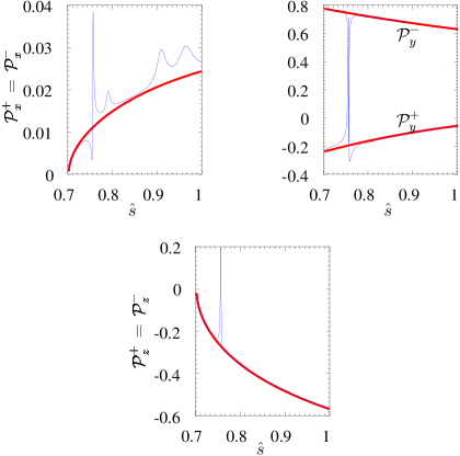
Figure 1: The polarization asymmetries for the $\tau^{-}$ and $\tau^{+}$, as functions of ${\hat{s}}$, the invariant mass of the $\tau$ pair, without (thick lines) and with (thin lines) the long-distance resonance contributions.

The coefficient ${\cal P}_{z}^{-}$ was computed in Ref. [4], ${\cal P}_{x}^{-}$, ${\cal P}_{y}^{-}$ and ${\cal P}_{z}^{-}$ were obtained in Ref. [5], and ${\cal P}_{x}^{+}$, ${\cal P}_{y}^{+}$ and ${\cal P}_{z}^{+}$ were calculated in Ref. [7]. (Note: while we agree with the calculations of Refs. [4, 5], we disagree with Ref. [7] about the expression for ${\cal P}_{y}^{\pm}$ [the equation following their Eq. (24)].) We plot the functions ${\cal P}_{x}^{-}$, ${\cal P}_{y}^{-}$ and ${\cal P}_{z}^{-}$ as functions of $\hat{s}$ in Fig. 1. For the purpose of numerical computations, we follow the prescription of Ref. [5] and include long-distance effects in $C_{9}^{eff}$ associated with real $c\bar{c}$ resonances in the intermediate states. We take the phenomenological parameter $\kappa_{V}$ multiplying the Breit-Wigner function in Ref. [5] to be unity.

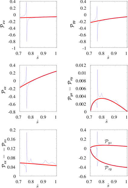
Figure 2: The double-spin polarization asymmetries, as functions of ${\hat{s}}$, the invariant mass of the $\tau$ pair, without (thick lines) and with (thin lines) the long-distance resonance contributions.

Note that our ${\cal P}_{z}^{-}$ is the same as the longitudinal polarization asymmetry of the $\tau^{-}$, $P_{L}^{-}$ of Refs. [5, 7]. However, ${\cal P}_{z}^{+}=-P_{L}^{+}$, since the $\tau^{+}$ moves along the $-\hat{z}$ axis. Similarly, ${\cal P}_{x}^{-}=P_{N}^{-}$ and ${\cal P}_{x}^{+}=-P_{N}^{+}$. (Note: the distribution of our $P_{N}$ differs from that of Ref. [5], resulting in a somewhat smaller value of $\langle P_{N}\rangle_{\tau}$.) The transverse direction defined in these references lies along the negative ${\hat{y}}$-direction for both $\tau^{-}$ and $\tau^{+}$, so that ${\cal P}_{y}^{-}=-P_{T}^{-}$ and ${\cal P}_{y}^{+}=-P_{T}^{+}$. The double-spin polarization asymmetries are shown in Fig. 2.

Previously, we noted that it is very likely that only asymmetries larger than 10% will be measurable. One characterization of the data is to calculate the average values of the above asymmetries. These are defined as

$$\langle{\cal P}\rangle\equiv\displaystyle\frac{\displaystyle\int^{1}_{4\,\hat{m}_{\tau}^{2}}{\cal P}\displaystyle\frac{d\Gamma}{d\hat{s}}d\hat{s}}{\displaystyle\int^{1}_{4\,\hat{m}_{\tau}^{2}}\displaystyle\frac{d\Gamma}{d\hat{s}}d\hat{s}}~{}.$$ (31)

In Table 1 we list the average values of all polarization asymmetries. From this Table, we see that only ${\cal P}_{y}^{\pm}$, ${\cal P}_{z}$, ${\cal P}_{yy}$, and ${\cal P}_{zy}$ can be considered sizeable. (Note that here, ${\cal P}_{z}^{+}={\cal P}_{z}^{-}\equiv{\cal P}_{z}$.)

$\langle{\cal P}_{x}^{-}\rangle=\langle{\cal P}_{x}^{+}\rangle$	$1.413\times 10^{-2}$
$\langle{\cal P}_{y}^{-}\rangle$	0.723
$\langle{\cal P}_{z}^{-}\rangle=\langle{\cal P}_{z}^{+}\rangle$	$-$0.336
$\langle{\cal P}_{y}^{+}\rangle$	$-$0.164
$\langle{\cal P}_{xx}\rangle$	$-8.658\times 10^{-2}$
$\langle{\cal P}_{yx}\rangle=\langle{\cal P}_{xy}\rangle$	$2.868\times 10^{-3}$
$\langle{\cal P}_{zx}\rangle=-\langle{\cal P}_{xz}\rangle$	$5.322\times 10^{-2}$
$\langle{\cal P}_{yy}\rangle$	$-$0.168
$\langle{\cal P}_{zy}\rangle$	$-$0.281
$\langle{\cal P}_{yz}\rangle$	$5.717\times 10^{-2}$
$\langle{\cal P}_{zz}\rangle$	$-1.1254\times 10^{-2}$

Table 1: Numerical values of the various averaged spin-polarization asymmetries without including the long-distance resonance contributions. We use $m_{b}=4.24$ GeV [8]. The corresponding branching ratio is $BR(B\to X_{s}\tau^{+}\tau^{-})=1.192\times 10^{-7}$.

In Eqs. (14)–(30), there are certain relations between the ${\cal P}$’s when the spins ${\bf s^{+}}$ and ${\bf s^{-}}$ are interchanged. Some of these relations are equalities, e.g. ${\cal P}_{x}^{-}={\cal P}_{x}^{+}$, ${\cal P}_{xz}={\cal P}_{zx}$, etc. For other pairs of ${\cal P}_{i}$’s, the expressions are similar, but only some of the terms change sign (e.g. ${\cal P}_{y}^{+}$ vs. ${\cal P}_{y}^{-}$). As we describe below, it is possible to understand these relations by considering also the conjugate process ${\bar{b}}\to{\bar{s}}\tau^{-}\tau^{+}$.

The processes $b\to s\tau^{+}\tau^{-}$ and ${\bar{b}}\to{\bar{s}}\tau^{-}\tau^{+}$ are related by CPT as follows [12]:

$$b(p_{b}) \to s(p_{s})\,\tau^{+}(p_{+},{\bf s_{+}})\,\tau^{-}(p_{-},{\bf s_{-}})~{},$$

$$\bar{b}(p_{b}) \to \bar{s}(p_{s})\,\tau^{-}(p_{+},-{\bf s_{+}})\,\tau^{+}(p_{-},-{\bf s_{-}})~{}.$$ (32)

In the absence of CP violation, observables which are P-odd must vanish in the (C-even) untagged sample. Consider first the terms involving triple-product (TP) correlations. While all triple products are T-odd, they can be either P-even or P-odd. Triple products involving two spins are necessarily P-odd and, in the absence of CP violation, C-odd. Because of this, in the SM, these triple product must vanish in the untagged sample. Thus, we have ${\rm TP}^{P-odd}_{\bar{b}}=-{\rm TP}^{P-odd}_{b}$. This relation can be violated in the presence of CP-violating new physics. On the other hand, triple products involving one spin are P-even and C-even, so that ${\rm TP}^{P-even}_{\bar{b}}=+{\rm TP}^{P-even}_{b}$, in the absence of CP violation. Thus, these triple products can survive in the untagged sample due to the presence of the strong phases which can fake CP-violating effects.

We now apply these observations to ${\cal P}_{x}^{+}$ and ${\cal P}_{x}^{-}$, which involve a single spin. As noted earlier, terms with a single spin along $\hat{x}$ must come only from a triple-product correlation. The general triple-product term giving these quantities can be written as $\epsilon_{\alpha\beta\mu\rho}\,p_{b}^{\alpha}p_{s}^{\beta}(a\,p_{+}^{\mu}s_{+}^{\rho}+b\,p_{-}^{\mu}s_{-}^{\rho})$, where $a$ and $b$ are arbitrary coefficients. For the conjugate process [Eq. (32)], the corresponding term is $-\epsilon_{\alpha\beta\mu\rho}\,p_{b}^{\alpha}p_{+}^{\beta}(a\,p_{-}^{\mu}s_{-}^{\rho}+b\,p_{+}^{\mu}s_{+}^{\rho})$. Since ${\rm TP}^{P-even}_{\bar{b}}=+{\rm TP}^{P-even}_{b}$, this implies that $a=-b$ (in the absence of CP violation). Using the 4-vectors of Eq. (6), it is then straightforward to show that this results in ${\cal P}_{x}^{+}=+{\cal P}_{x}^{-}$. Note that this will hold even in the presence of CP-conserving New Physics.

Similarly, the two-spin triple products, which contribute to the pairs $\{{\cal P}_{yx},{\cal P}_{xy}\}$ and $\{{\cal P}_{zx},{\cal P}_{xz}\}$, are proportional to $\epsilon_{\alpha\beta\mu\rho}\,p_{s}^{\alpha}p_{b}^{\beta}s_{-}^{\mu}s_{+}^{\rho}$. In the absence of CP violation, the CP-odd combination of ${\cal P}_{yx}$ and ${\cal P}_{xy}$ (and of ${\cal P}_{zx}$ and ${\cal P}_{xz}$) will vanish in an untagged sample. Again, a simple calculation then shows that this implies that ${\cal P}_{yx}=+{\cal P}_{xy}$ and ${\cal P}_{zx}=-{\cal P}_{xz}$.

For the other terms that do not contain triple products, and are hence always T-even, one can understand the relationship between the ${\cal P}$’s in a similar fashion. For example, consider ${\cal P}_{y}^{+}$ and ${\cal P}_{y}^{-}$. Since only dot products of various momenta and one spin are involved, the coefficients of both terms $|C_{7}^{eff}|^{2}$ [Eq. (54)] and ${\rm Re}(C_{7}^{eff}C_{10}^{*})$ [Eq. (56)] are T-even and P-odd. However, the $|C_{7}^{eff}|^{2}$ term “$p_{s}\cdot(s^{-}+s^{+})$” switches sign under CPT for the conjugate process, while the ${\rm Re}(C_{7}^{eff}C_{10}^{*})$ term “$p_{s}\cdot(s^{+}-s^{-})$” has the same sign for the conjugate process. Since these terms are P-odd and C-odd (in the absence of CP violation), they must vanish in an untagged sample. This explains the relative sign difference between the $|C_{7}^{eff}|^{2}$ and ${\rm Re}(C_{7}^{eff}C_{10}^{*})$ terms in ${\cal P}_{y}^{+}$ and ${\cal P}_{y}^{-}$. This argument may be extended to all terms contributing to various ${\cal P}_{i}$’s. In particular, in the SM, ${\cal P}_{z}^{+}=+{\cal P}_{z}^{-}$. On the other hand, in presence of New Physics, while the additional terms must still be T-even and P-odd, they could be even or odd under CPT, implying that the relation between ${\cal P}_{z}^{+}$ and ${\cal P}_{z}^{-}$ could differ.

Of course, the above discussion assumes that there is no CP violation in $b\to s\tau^{+}\tau^{-}$, which is the case in the SM, to a good approximation. On the other hand, if new CP-violating physics contributes to this decay, this gives us several clear tests for its presence. For example, any violation of the relation ${\cal P}_{x}^{+}={\cal P}_{x}^{-}$ (or $P_{L}^{-}+P_{L}^{+}=0$) is a smoking-gun signal of such new physics.

4 Forward-Backward Asymmetries

One observable which does not depend on the polarization of the final-state leptons is the forward-backward (FB) asymmetry. In the frame of reference described in Eq. (6), the forward-backward asymmetry is given by

$$A_{FB}(\hat{s}) = \displaystyle\frac{\displaystyle\int_{0}^{1}\frac{d^{2}\Gamma}{d\hat{s}~{}d\cos\theta}d\cos\theta-\int_{-1}^{0}\frac{d^{2}\Gamma}{d\hat{s}~{}d\cos\theta}d\cos\theta}{\displaystyle\int_{0}^{1}\frac{d^{2}\Gamma}{d\hat{s}~{}d\cos\theta}d\cos\theta+\int_{-1}^{0}\frac{d^{2}\Gamma}{d\hat{s}~{}d\cos\theta}d\cos\theta}$$ (33)

$$= \frac{3}{\Delta}\,\Big{(}2\,{{\rm Re}(C_{7}^{eff}C_{10}^{*})}\,+\hat{s}\,{{\rm Re}(C_{9}^{eff}C_{10}^{*})}\Big{)}\,\sqrt{1-\frac{4\,\hat{m}_{\tau}^{2}}{\hat{s}}}~{}.$$

This agrees with the result of Ref. [5] (and that of Ref. [11] when $m_{\tau}$ is neglected). Note that the FB asymmetry is of opposite sign for the CP-conjugate process ${\bar{b}}\to{\bar{s}}\tau^{+}\tau^{-}$, so that $A_{FB}^{b}+A_{FB}^{\bar{b}}=0$. Thus, in order to measure the unpolarized FB asymmetry, it will be necessary to tag the flavor of the decaying $b$-quark.

If the polarization of the final-state leptons can be measured, then, in addition to the polarization asymmetries discussed in the previous section, one can also extract forward-backward asymmetries of the polarized leptons. While the unpolarized FB asymmetry of Eq. (33) requires $b$-tagging, some of the polarized FB asymmetries are non-vanishing even in an untagged sample.

We can extract the forward-backward asymmetries corresponding to various polarization components of the $\tau^{-}$ and/or $\tau^{+}$ spin by writing:

$$A_{FB}({\bf s^{+}},{\bf s^{-}},\hat{s}) = A_{FB}(\hat{s})+\Big{[}{\cal A}^{-}_{x}s_{x}^{-}+{\cal A}^{-}_{y}s_{y}^{-}+{\cal A}^{-}_{z}s_{z}^{-}+{\cal A}^{+}_{x}s_{x}^{+}+{\cal A}^{+}_{y}s_{y}^{+}+{\cal A}^{+}_{z}s_{z}^{+}$$ (34)

$$\hskip 72.26999pt+~{}{\cal A}_{xx}s_{x}^{+}s_{x}^{-}+{\cal A}_{xy}s_{x}^{+}s_{y}^{-}+{\cal A}_{xz}s_{x}^{+}s_{z}^{-}$$

$$\hskip 72.26999pt+~{}{\cal A}_{yx}s_{y}^{+}s_{x}^{-}+{\cal A}_{yy}s_{y}^{+}s_{y}^{-}+{\cal A}_{yz}s_{y}^{+}s_{z}^{-}$$

$$\hskip 72.26999pt+~{}{\cal A}_{zx}s_{z}^{+}s_{x}^{-}+{\cal A}_{zy}s_{z}^{+}s_{y}^{-}+{\cal A}_{zz}s_{z}^{+}s_{z}^{-}\Big{]}~{}.$$

The various polarized forward-backward asymmetries are then evaluated to be

$${\cal A}^{+}_{x} = 0$$ (35)

$${\cal A}^{+}_{y} = \frac{2}{\Delta}\,{{\rm Re}(C_{9}^{eff}C_{10}^{*})}\,\frac{(1-\hat{s})\,\hat{m}_{\tau}}{\sqrt{\hat{s}}}\,\sqrt{1-\frac{4\,\hat{m}_{\tau}^{2}}{\hat{s}}}$$ (36)

$${\cal A}^{+}_{z} = \frac{1}{\Delta}\Bigg{(}6\,{{\rm Re}(C_{7}^{eff}C_{9}^{eff^{*}})}-\frac{6\,|C_{7}^{eff}|^{2}}{\hat{s}}-3\,(\,|C_{9}^{eff}|^{2}-|C_{10}|^{2})\,\hat{m}_{\tau}^{2}$$ (37)

$$-12\,{{\rm Re}(C_{7}^{eff}C_{10}^{*})}\,\frac{\hat{m}_{\tau}^{2}}{\hat{s}}-~{}6\,{{\rm Re}(C_{9}^{eff}C_{10}^{*})}\,\frac{\hat{m}_{\tau}^{2}}{\hat{s}}$$

$$-~{}\frac{3}{2}\,(\,|C_{9}^{eff}|^{2}+|C_{10}|^{2})\,\hat{s}\,(1-\frac{2\,\hat{m}_{\tau}^{2}}{\hat{s}})\Bigg{)}$$

$${\cal A}^{-}_{x} = 0$$ (38)

$${\cal A}^{-}_{y} = {\cal A}^{+}_{y}$$ (39)

$${\cal A}^{-}_{z} = \frac{1}{\Delta}\Bigg{(}-6\,{{\rm Re}(C_{7}^{eff}C_{9}^{eff^{*}})}-\frac{6\,|C_{7}^{eff}|^{2}}{\hat{s}}-3\,(\,|C_{9}^{eff}|^{2}-|C_{10}|^{2})\,\hat{m}_{\tau}^{2}$$ (40)

$$+~{}12\,{{\rm Re}(C_{7}^{eff}C_{10}^{*})}\,\frac{\hat{m}_{\tau}^{2}}{\hat{s}}+~{}6\,{{\rm Re}(C_{9}^{eff}C_{10}^{*})}\,\frac{\hat{m}_{\tau}^{2}}{\hat{s}}$$

$$-~{}\frac{3}{2}\,(\,|C_{9}^{eff}|^{2}+|C_{10}|^{2})\,\hat{s}\,(1-\frac{2\,\hat{m}_{\tau}^{2}}{\hat{s}})\Bigg{)}$$

$${\cal A}_{xx} = 0$$ (41)

$${\cal A}_{xy} = \frac{-6}{\Delta}\,(2\,{{\rm Im}(C_{7}^{eff}\,C_{10}^{*})}+{{\rm Im}(C_{9}^{eff}\,C_{10}^{*})})\,\frac{{{\hat{m}_{\tau}}}^{2}}{\hat{s}}$$ (42)

$${\cal A}_{xz} = \frac{2}{\Delta}\,{{\rm Im}(C_{9}^{eff}C_{10}^{*})}\,\frac{(1-\hat{s})\,{\hat{m}_{\tau}}}{\sqrt{\hat{s}}}\,\sqrt{1-\frac{4\,\hat{m}_{\tau}^{2}}{\hat{s}}}$$ (43)

$${\cal A}_{yx} = -{\cal A}_{xy}$$ (44)

$${\cal A}_{yy} = 0$$ (45)

$${\cal A}_{yz}\! = \!\Big{(}2|C_{9}^{eff}|^{2}-\frac{8\,|C_{7}^{eff}|^{2}}{\hat{s}}\Big{)}\,\frac{(1-\hat{s})\,\hat{m}_{\tau}}{\Delta\sqrt{\hat{s}}}$$ (46)

$${\cal A}_{zx} = {\cal A}_{xz}$$ (47)

$${\cal A}_{zy} = {\cal A}_{yz}$$ (48)

$${\cal A}_{zz} = \frac{-3}{\Delta}\,(2\,{{\rm Re}(C_{7}^{eff}\,C_{10}^{*})}+{{\rm Re}(C_{9}^{eff}\,C_{10}^{*})}\,\hat{s})\,{\sqrt{1-\frac{4\,{{\hat{m}_{\tau}}}^{2}}{\hat{s}}}}~{}.$$ (49)

Note that, in the SM, it turns out that $A_{FB}=-{\cal A}_{zz}$.

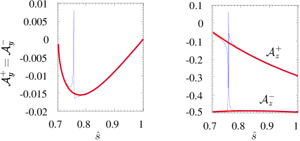
Figure 3: Forward-backward asymmetries of the $\tau^{-}$ and $\tau^{+}$, as functions of ${\hat{s}}$, the invariant mass of the $\tau$ pair, without (thick lines) and with (thin lines) the long-distance resonance contributions.

The nonzero single-spin forward-backward asymmetries are depicted in Fig. 3 as functions of $\hat{s}$, while those with both spins polarized are shown in Fig. 4. Interestingly, some of the forward-backward asymmetries are identically zero within the SM: ${\cal A}_{x}^{+}$, ${\cal A}_{x}^{-}$, ${\cal A}_{xx}$ and ${\cal A}_{yy}$. Nonvanishing values of these asymmetries would be clear signals of NP. Also, as was discussed in the case of the polarization asymmetries, the discrete transformation properties of the operators can once again be used to understand the relations between pairs of forward-backward asymmetries in which the spins ${\bf s^{+}}$ and ${\bf s^{-}}$ are interchanged.

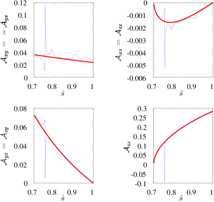
Figure 4: Doubly-polarized forward-backward asymmetries, as functions of ${\hat{s}}$, the invariant mass of the $\tau$ pair, without (thick lines) and with (thin lines) the long-distance resonance contributions.

The average values of the forward-backward asymmetries are defined similarly to Eq. (31) and are listed in Table 2. From this table, we see that only three asymmetries are expected to be larger than 10% in the SM: ${\cal A}_{z}^{\pm}$ and ${\cal A}_{zz}$.

$\langle{\cal A}_{y}^{+}\rangle=\langle{\cal A}_{y}^{-}\rangle$	$-1.302\times 10^{-2}$
$\langle{\cal A}_{z}^{+}\rangle$	$-$0.148
$\langle{\cal A}_{z}^{-}\rangle$	$-$0.490
$\langle{\cal A}_{xy}\rangle=-\langle{\cal A}_{yx}\rangle$	$3.184\times 10^{-2}$
$\langle{\cal A}_{xz}\rangle=\langle{\cal A}_{zx}\rangle$	$-1.347\times 10^{-3}$
$\langle{\cal A}_{yz}\rangle=\langle{\cal A}_{zy}\rangle$	$4.298\times 10^{-2}$
$\langle{\cal A}_{zz}\rangle$	0.154

Table 2: Numerical values of the various average polarized forward-backward asymmetries without including the long distance resonance contributions. We use $m_{b}=4.24$ GeV [8]. The corresponding average unpolarized forward-backward asymmetry is $\langle A_{FB}\rangle=-0.154$.

5 Discussion

In the previous sections, we have discussed the polarization and forward-backward asymmetries which can be obtained when the spins of the $\tau^{+}$ and/or $\tau^{-}$ are measured. Here we consider what can be learned from these measurements in a variety of scenarios.

First, suppose that the statistics are such that only a single polarization can be measured (say that of the $\tau^{-}$), and that no tagging is possible. In this case only the P-even observables survive: ${\cal P}_{x}^{+}+{\cal P}_{x}^{-}$, ${\cal A}_{y}^{+}+{\cal A}_{y}^{-}$ and ${\cal A}_{z}^{+}+{\cal A}_{z}^{-}$. Of these asymmetries only ${\cal A}_{z}^{+}+{\cal A}_{z}^{-}$ is measurable within the SM. Along with the differential decay rate, this therefore gives only two observables, which is not enough to test the SM.

On the other hand, if the polarizations of both $\tau^{+}$ and $\tau^{-}$ can be measured, still without tagging, then one adds another six observables: ${\cal P}_{xx}$, ${\cal P}_{yy}$, ${\cal P}_{zy}+{\cal P}_{yz}$, ${\cal P}_{zz}$, ${\cal A}_{xy}+{\cal A}_{yx}$, and ${\cal A}_{xz}+{\cal A}_{zx}$. Of these only three — ${\cal P}_{yy}$, ${\cal P}_{zy}+{\cal P}_{yz}$ and ${\cal P}_{zz}$ — are expected to be sizeable in the SM, the last one being measurable only as a distribution in $\hat{s}$ (see Fig. 2). We therefore have just enough measurements to determine the five unknowns $C_{7}^{eff}$, $C_{10}$, ${\rm Re}(C_{9}^{eff})$, ${\rm Im}(C_{9}^{eff})$, and $m_{b}$. However, there are not enough measurements to provide an internal crosscheck of the predictions of the SM.

Now suppose that it is possible to tag the flavor of the decaying $b$-quark. If only a single $\tau$-spin measurement is performed then, out of a total of thirteen possible asymmetries, only six are sizeable within the SM: ${\cal A}_{FB}$, ${\cal P}_{y}^{\pm}$, ${\cal P}_{z}$ and ${\cal A}_{z}^{\pm}$. (Recall that ${\cal P}_{z}^{+}={\cal P}_{z}^{-}\equiv{\cal P}_{z}$.)

In the best-case scenario, it will be possible to both tag the flavor of the decaying $b$, and to measure the polarizations of both final-state $\tau$ leptons. In this case, one in principle has 31 asymmetries. However, within the SM only nine of these are accessible: ${\cal A}_{FB}$, ${\cal P}_{y}^{\pm}$, ${\cal P}_{z}$, ${\cal A}_{z}^{\pm}$, ${\cal P}_{yy}$, ${\cal P}_{zy}$ and ${\cal A}_{zz}$. Even so, if these asymmetries could be measured, this would allow us to greatly overconstrain the SM. Ideally, we will find evidence for new physics, but if not, these will provide precision determinations of both $m_{b}$ and the Wilson coefficients describing the decay $b\to s\tau^{+}\tau^{-}$.

In Table 3 we summarize the number of possible observables, including the differential cross-section, in the various scenarios discussed above.

		Untagged Sample	Tagged Sample
Only one of $\tau^{+}$ or $\tau^{-}$ spin measured		$\frac{d\Gamma}{d\hat{s}}$, ${\cal P}_{x}^{(\pm)}$, ${\cal A}_{y}^{(\pm)}$, ${\cal A}_{z}^{(\pm)}$[4]	$\frac{d\Gamma}{d\hat{s}}$, ${\cal A}_{FB}$, ${\cal P}_{x}^{\pm}$, ${\cal P}_{y}^{\pm}$, ${\cal P}_{z}^{\pm}$, ${\cal A}_{x}^{\pm}$, ${\cal A}_{y}^{\pm}$, ${\cal A}_{z}^{\pm}$ [14]
	SM	$\frac{d\Gamma}{d\hat{s}}$, ${\cal A}_{z}^{(\pm)}$ [2]	$\frac{d\Gamma}{d\hat{s}}$, ${\cal A}_{FB}$, ${\cal P}_{y}^{\pm}$, ${\cal P}_{z}$, ${\cal A}_{z}^{\pm}$ [7]
Both $\tau^{+}$ and $\tau^{-}$ spins measured		$+$ ${\cal P}_{xx}$, ${\cal P}_{yy}$, ${\cal P}_{(zy)}$, ${\cal P}_{zz}$, ${\cal A}_{(xy)}$, ${\cal A}_{(xz)}$ [10]	All [32]
	SM	$+$ ${\cal P}_{yy}$, ${\cal P}_{(zy)}$, ${\cal P}_{zz}$ [5]	$+$ ${\cal P}_{yy}$, ${\cal P}_{zy}$, ${\cal P}_{zz}$ [10]

Table 3: The number of observables in various scenarios of initial $b$-flavor tagging and $\tau$-spin measurements. The columns represent the cases with untagged and tagged samples, while the rows are for the scenarios in which only one of the $\tau^{+}$ or $\tau^{-}$ spin is measured, or when both $\tau^{+}$ and $\tau^{-}$ spins are measured. Of the possible observables, those that are sizeable in the SM are listed separately. In the case in which both spins are measured, only the additional observables (indicated by $+$) are listed. The number in the square brackets represents the total number of observables possible in each case. $\mathcal{P}_{(ij)}$ indicates the sum $\mathcal{P}_{ij}+\mathcal{P}_{ji}$ and $\mathcal{P}^{(\pm)}_{i}=\mathcal{P}^{+}_{i}+\mathcal{P}^{-}_{i}$, with identical definitions for the $\mathcal{A}$’s.

Finally, we note that in some of these scenarios, it will be possible to extract the value of $m_{b}$. This is advantageous for two reasons. First, it permits a direct comparison with the theoretical estimates of $m_{b}$ [8]. Second, for some measurements in the $B$ system, it is necessary to input $m_{b}$ from theory, which increases the systematic (theoretical) uncertainty of the measurement. By contrast, we see that the double-spin analysis of $b\to s\tau^{+}\tau^{-}$ will not suffer from this type of systematic error.

6 Conclusions

In the standard model (SM), the inclusive decay $b\to s\tau^{+}\tau^{-}$ is described by five theoretical parameters: $C_{7}^{eff}$, $C_{10}$, ${\rm Re}(C_{9}^{eff})(\hat{s})$, ${\rm Im}(C_{9}^{eff})(\hat{s})$ and $m_{b}$, where $\hat{s}$ is related to the momentum transferred to the lepton pair. We would like to be able to test this description.

In this paper, we have calculated all single- and double-spin asymmetries in the decay $b\to s\tau^{+}\tau^{-}$. We have shown that there are many different ways of testing the SM description of this decay. In all, there are a total of 31 different asymmetries. However, only 9 of these are predicted to be measurable, i.e. have values larger than 10%. (Indeed some asymmetries are expected to vanish in the SM.) Should any of the small asymmetries be found to have large values, this would be a clear signal of new physics (NP). Furthermore, the SM predicts certain relationships among the asymmetries when the spins ${\bf s^{+}}$ and ${\bf s^{-}}$ are interchanged. Should these relations be violated, this would also indicate the presence of NP. In fact, this could give us some clue as to whether the NP is CP-conserving or CP-violating.

Apart from these signals of NP, whether or not the SM can be tested depends crucially on which types of measurements can be made. For example, if one cannot perform $b$-tagging, and can measure only a single individual $\tau$ spin, then there are only two sizeable observables. This is not enough to test the SM. On the other hand, if one can measure both $\tau$ spins, but cannot tag the flavor of the $b$, then there are a total of five measurable observables. This is enough to determine the theoretical unknowns, but does not provide the necessary redundancy to test the SM.

On the other hand, if one can perform $b$-tagging, but can only measure a single $\tau$ spin, then there are 7 sizeable observables. This can provide a redundant test of the SM. The optimal scenario is if $b$-tagging is possible, and one can measure the polarizations of both the $\tau^{+}$ and $\tau^{-}$. In this case, there are a total of 10 independent measurements, which would greatly overconstrain the SM. If new physics is not found, this would precisely determine the five theoretical parameters.

Note that testing the SM implies that the quantity $m_{b}$ will be extracted from the experimental data. This will allow us to compare the experimental value of $m_{b}$ with the theoretical estimates of this same quantity. Furthermore, as the measurements do not rely on theoretical input, the systematic error will be correspondingly reduced.

Acknowledgements: N.S. and R.S. thank D.L. for the hospitality of the Université de Montréal, where part of this work was done. The work of D.L. was financially supported by NSERC of Canada. The work of Nita Sinha was supported by a project of the Department of Science and Technology, India, under the young scientist scheme.

7 Appendix

In this Appendix, we calculate the square of the amplitude in Eq. (1), keeping the spins of both final-state leptons. We define $p_{b}$, $p_{s}$, $p_{+}$ and $p_{-}$ to be the momenta of the $b$-quark, $s$-quark, $\tau^{+}$ and $\tau^{-}$, respectively, with $q=p_{b}-p_{s}=p_{+}+p_{-}$. The spins of the $\tau^{+}$ and $\tau^{-}$ are denoted by $s_{+}$ and $s_{-}$, respectively. We have

$${|\cal M|}^{2}=|T_{9}|^{2}+|T_{10}|^{2}+|T_{7}|^{2}+2{\rm Re}\left(T_{9}^{\dagger}T_{10}\right)+2{\rm Re}\left(T_{9}^{\dagger}T_{7}\right)+2{\rm Re}\left(T_{10}^{\dagger}T_{7}\right)~{}.$$ (50)

Summing over the $s$-quark spin and averaging over the $b$-quark spin, We find

$${1\over 2}\sum_{b,s\ spins}|T_{9}|^{2} = {\alpha^{2}G_{F}^{2}\over\pi^{2}}|V_{tb}V_{ts}^{*}|^{2}|C_{9}^{eff}|^{2}$$ (51)

$$\times \left\{{(m_{b}^{2}-q^{2})\over 2}\left(-p_{-}\cdot s_{+}\,p_{+}\cdot s_{-}+{q^{2}\over 2}s_{+}\cdot s_{-}+m_{\tau}^{2}(1-s_{+}\cdot s_{-})\right)\right.$$

$$+(1-s_{+}\cdot s_{-})\left(p_{b}\cdot p_{+}\,p_{s}\cdot p_{-}+p_{s}\cdot p_{+}\,p_{b}\cdot p_{-}\right)$$

$$-{q^{2}\over 2}\left[p_{b}\cdot s_{+}\,p_{s}\cdot s_{-}+p_{s}\cdot s_{+}\,p_{b}\cdot s_{-}\right]$$

$$+s_{+}\cdot p_{-}\left[p_{b}\cdot p_{+}\,p_{s}\cdot s_{-}+p_{s}\cdot p_{+}\,p_{b}\cdot s_{-}\right]$$

$$+s_{-}\cdot p_{+}\left[p_{b}\cdot p_{-}\,p_{s}\cdot s_{+}+p_{s}\cdot p_{-}\,p_{b}\cdot s_{+}\right]$$

$$+m_{\tau}\bigg{[}p_{s}\cdot(p_{+}+p_{-})\,p_{b}\cdot(s_{+}+s_{-})$$

$$\hskip 42.67912pt-p_{b}\cdot(p_{+}+p_{-})\,p_{s}\cdot(s_{+}+s_{-})\bigg{]}\Bigg{\}}~{},$$

$${1\over 2}\sum_{b,s\ spins}|T_{10}|^{2} = {\alpha^{2}G_{F}^{2}\over\pi^{2}}|V_{tb}V_{ts}^{*}|^{2}|C_{10}|^{2}$$ (52)

$$\times \left\{-{(m_{b}^{2}-q^{2})\over 2}\left(-p_{-}\cdot s_{+}\,p_{+}\cdot s_{-}+{q^{2}\over 2}s_{+}\cdot s_{-}+m_{\tau}^{2}(1-s_{+}\cdot s_{-})\right)\right.~{}$$

$$+(1+s_{+}\cdot s_{-})\left(p_{b}\cdot p_{+}\,p_{s}\cdot p_{-}+p_{s}\cdot p_{+}\,p_{b}\cdot p_{-}\right)~{}$$

$$-\left(2m_{\tau}^{2}-{q^{2}\over 2}\right)\left[p_{b}\cdot s_{+}\,p_{s}\cdot s_{-}+p_{s}\cdot s_{+}\,p_{b}\cdot s_{-}\right]~{}$$

$$-s_{+}\cdot p_{-}\left[p_{b}\cdot p_{+}\,p_{s}\cdot s_{-}+p_{s}\cdot p_{+}\,p_{b}\cdot s_{-}\right]~{}$$

$$-s_{-}\cdot p_{+}\left[p_{b}\cdot p_{-}\,p_{s}\cdot s_{+}+p_{s}\cdot p_{-}\,p_{b}\cdot s_{+}\right]~{}$$

$$-m_{\tau}\bigg{[}p_{s}\cdot(p_{+}-p_{-})\,p_{b}\cdot(s_{+}-s_{-})$$

$$\hskip 42.67912pt-p_{b}\cdot(p_{+}-p_{-})\,p_{s}\cdot(s_{+}-s_{-})\bigg{]}\Bigg{\}}~{},$$

$$\sum_{b,s\ spins}{\rm Re}\Big{[}T_{9}^{\dagger}T_{10}\Big{]} = {\alpha^{2}G_{F}^{2}\over\pi^{2}}|V_{tb}V_{ts}^{*}|^{2}$$ (53)

$$\times \Bigg{\{}2{\rm Re}(C_{9}^{eff}C_{10}^{\ast})\bigg{[}m_{\tau}^{2}\big{[}p_{s}\cdot s_{-}\,p_{b}\cdot s_{+}-p_{b}\cdot s_{-}\,p_{s}\cdot s_{+}\big{]}$$

$$\hskip 14.22636pt-{q^{2}\over 2}(p_{s}\cdot p_{-}-p_{s}\cdot p_{+})~{}$$

$$\hskip 14.22636pt+m_{\tau}\big{[}p_{b}\cdot p_{+}\,p_{s}\cdot s_{-}+p_{s}\cdot p_{+}\,p_{b}\cdot s_{-}$$

$$\hskip 14.22636pt-p_{b}\cdot p_{-}\,p_{s}\cdot s_{+}-p_{s}\cdot p_{-}\,p_{b}\cdot s_{+}\big{]}\bigg{]}~{}$$

$$+{\rm Im}(C_{9}^{eff}C_{10}^{\ast}){\epsilon}_{\mu\alpha\beta\phi}\bigg{[}\Big{[}2m_{\tau}+(p_{s}+p_{b})\cdot s_{+}\Big{]}p_{s}^{\mu}p_{-}^{\alpha}s_{-}^{\beta}p_{+}^{\phi}~{}$$

$$\hskip 14.22636pt-\Big{[}2m_{\tau}+(p_{s}+p_{b})\cdot s_{-}\Big{]}p_{s}^{\mu}p_{+}^{\alpha}s_{+}^{\beta}p_{-}^{\phi}~{}$$

$$\hskip 14.22636pt-(p_{s}+p_{b})\cdot p_{+}\,p_{s}^{\mu}p_{-}^{\alpha}s_{-}^{\beta}s_{+}^{\phi}+(p_{s}+p_{b})\cdot p_{-}\,p_{s}^{\mu}p_{+}^{\alpha}s_{+}^{\beta}s_{-}^{\phi}~{}$$

$$\hskip 14.22636pt+(p_{-}-p_{+})\cdot p_{s}\,p_{-}^{\mu}p_{+}^{\alpha}s_{+}^{\beta}s_{-}^{\phi}\bigg{]}\Bigg{\}}~{},$$

$${1\over 2}\sum_{b,s\ spins}|T_{7}|^{2} = {\alpha^{2}G_{F}^{2}\over\pi^{2}}|V_{tb}V_{ts}^{*}|^{2}{m_{b}^{2}\over q^{4}}|C_{7}|^{2}$$ (54)

$$\times \Bigg{\{}4m_{b}^{2}m_{\tau}\bigg{[}p_{s}\cdot(p_{+}+p_{-})\,q\cdot(s_{-}+s_{+})-q^{2}\,p_{s}\cdot(s_{-}+s_{+})\bigg{]}~{}$$

$$+2m_{\tau}^{2}m_{b}^{2}(m_{b}^{2}-q^{2})\big{[}(1-s_{+}\cdot s_{-}\big{]}+q^{2}m_{b}^{2}(m_{b}^{2}-q^{2})~{}$$

$$-2q^{2}\bigg{[}2\big{[}p_{s}\cdot p_{-}\,p_{b}\cdot p_{+}+p_{s}\cdot p_{+}\,p_{b}\cdot p_{-}\big{]}-q^{2}\,p_{b}\cdot p_{s}\bigg{]}\big{[}(1-s_{+}\cdot s_{-}\big{]}~{}$$

$$-4q^{2}\bigg{[}s_{+}\cdot p_{-}\big{[}p_{s}\cdot s_{-}\,p_{b}\cdot p_{+}+p_{b}\cdot s_{-}\,p_{s}\cdot p_{+}\big{]}$$

$$\hskip 28.45274pt+s_{-}\cdot p_{+}\big{[}p_{s}\cdot p_{-}\,p_{b}\cdot s_{+}+p_{b}\cdot p_{-}\,p_{s}\cdot s_{+}\big{]}\bigg{]}~{}$$

$$+2q^{2}(m_{b}^{2}-q^{2})\,s_{+}\cdot p_{-}\,s_{-}\cdot p_{+}$$

$$+2q^{4}\big{[}p_{s}\cdot s_{-}\,p_{b}\cdot s_{+}+p_{b}\cdot s_{-}\,p_{s}\cdot s_{+}\big{]}\Bigg{\}}~{},$$

$$\sum_{b,s\ spins}{\rm Re}\Big{[}T_{9}^{\dagger}T_{7}\Big{]} = {\alpha^{2}G_{F}^{2}\over\pi^{2}}|V_{tb}V_{ts}^{*}|^{2}{m_{b}^{2}\over q^{2}}$$ (55)

$$\times \Bigg{\{}{\rm Re}(C_{9}^{eff}c_{7}^{\ast})\bigg{[}(m_{b}^{2}-q^{2})\big{[}q^{2}+2m_{\tau}^{2}-2m_{\tau}^{2}\,s_{+}\cdot s_{-}\big{]}$$

$$-4m_{\tau}\big{[}p_{b}\cdot(p_{+}+p_{-})\,p_{s}\cdot(s_{+}+s_{-})$$

$$\hskip 28.45274pt-p_{s}\cdot(p_{+}+p_{-})\,p_{b}\cdot(s_{+}+s_{-})\big{]}\bigg{]}\Bigg{\}}~{},$$

$$\sum_{b,s\ spins}{\rm Re}\Big{[}T_{10}^{\dagger}T_{7}\Big{]} = {\alpha^{2}G_{F}^{2}\over\pi^{2}}|V_{tb}V_{ts}^{*}|^{2}{m_{b}^{2}\over q^{2}}~{}$$ (56)

$$\times \Bigg{\{}-2{\rm Re}(C_{10}C_{7}^{eff^{*}})\bigg{[}-{m_{\tau}(m_{b}^{2}-q^{2})\over 2}\big{[}p_{+}\cdot s_{-}-p_{-}\cdot s_{+}\big{]}~{}$$

$$+q^{2}\big{[}p_{s}\cdot p_{-}-p_{s}\cdot p_{+}\big{]}-2m_{\tau}^{2}\big{[}p_{s}\cdot s_{-}\,p_{-}\cdot s_{+}-p_{+}\cdot s_{-}\,p_{s}\cdot s_{+}\big{]}~{}$$

$$+m_{\tau}\,q^{2}p_{s}\cdot(s_{+}-s_{-})+m_{\tau}\,p_{s}\cdot(p_{-}-p_{+})(s_{-}\cdot p_{+}+s_{+}\cdot p_{-})\bigg{]}~{}$$

$$-4{\rm Im}(C_{10}C_{7}^{eff^{*}}){\epsilon}_{\alpha\beta\mu\rho}\bigg{[}-m_{\tau}\,p_{s}^{\alpha}p_{+}^{\beta}s_{+}^{\mu}p_{b}^{\rho}+m_{\tau}\,p_{s}^{\alpha}p_{-}^{\beta}s_{-}^{\mu}p_{b}^{\rho}$$

$$\qquad+m_{\tau}^{2}\,s_{-}^{\alpha}p_{s}^{\beta}s_{+}^{\mu}p_{b}^{\rho}\bigg{]}\Bigg{\}}~{}.$$

In the above, we have used the convention $\epsilon_{0123}=+1$. Note that, as mentioned in Sec. 2, $C_{7}^{eff}$ and $C_{10}$ are expected to be real; only $C_{9}^{eff}$ is complex. However, in the expressions above, for completeness we have included both real and imaginary pieces of all Wilson coefficients.

References

[1] W. S. Hou, R. S. Willey and A. Soni, Phys. Rev. Lett. 58, 1608 (1987) [Erratum-ibid. 60, 2337 (1988)];
N. G. Deshpande and J. Trampetic, Phys. Rev. Lett. 60, 2583
(1988); A. Ali, T. Mannel and T. Morozumi, Phys. Lett. B 273, 505 (1991); A. F. Falk, M. E. Luke and M. J. Savage, Phys. Rev. D 49, 3367 (1994); A. Ali, G. F. Giudice and T. Mannel,
Zeit. Phys. C67, 417 (1995); C. Greub, A. Ioannisian and D. Wyler, Phys. Lett. B 346, 149 (1995); J. L. Hewett, Phys. Rev. D53, 4964 (1996);
F. Kruger and L. M. Sehgal, Phys. Lett. 380B, 199 (1996); A. Ali, G. Hiller,
L. T. Handoko and T. Morozumi, Phys. Rev. D 55, 4105 (1997);
C. S. Kim, T. Morozumi and A. I. Sanda, Phys. Rev. D 56,
7240 (1997); T. M. Aliev, C. S. Kim and M. Savci, Phys. Lett. B
441, 410 (1998); C. Q. Geng and C. P. Kao, Phys. Rev. D 57, 4479 (1998); S. Fukae, C. S. Kim, T. Morozumi and T. Yoshikawa,
Phys. Rev. D 59, 074013 (1999); Y. G. Kim, P. Ko and
J. S. Lee, Nucl. Phys. B 544, 64 (1999); S. Fukae, C. S. Kim
and T. Yoshikawa, Phys. Rev. D61, 074015 (2000); M. Zhong, Y. L. Wu and
W. Y. Wang, arXiv:hep-ph/0206013; A. Ghinculov, T. Hurth, G. Isidori
and Y. P. Yao, arXiv:hep-ph/0208088; H. M. Asatrian, K. Bieri,
C. Greub and A. Hovhannisyan, arXiv:hep-ph/0209006.
[2] P. L. Cho, M. Misiak and D. Wyler, Phys. Rev. D
54, 3329 (1996); Y. Grossman, Z. Ligeti and E. Nardi, Phys. Rev. D 55, 2768 (1997); J. L. Hewett and J. D. Wells, Phys. Rev. D 55, 5549 (1997); T. Goto, Y. Okada, Y. Shimizu and
M. Tanaka, Phys. Rev. D 55, 4273 (1997) [Erratum-ibid. D
66, 019901 (2002)]; L. T. Handoko, Nuovo Cim. A 111, 95
(1998); J. H. Jang, Y. G. Kim and J. S. Lee, Phys. Rev. D 58, 035006 (1998); T. G. Rizzo, Phys. Rev. D 58, 114014
(1998); S. Rai Choudhury, A. Gupta and N. Gaur, Phys. Rev. D 60, 115004 (1999); C.-S. Huang and S. H. Zhu, Phys. Rev. D 61, 015011 (2000) [Erratum-ibid. D 61, 119903 (2000)].
[3] A. Ali, G. F. Giudice and T. Mannel, Ref. [1].
[6] Refs. [5] and [7] give and ,
respectively. The authors of Ref. [7] cut out resonances
below the , which increases the asymmetry, while the authors
of Ref. [5] have used a cut of MeV for the
resonances. As we show later in the paper, we find .
[7] S. Fukae, C. S. Kim and T. Yoshikawa, Ref. [1].
[8] A.X. El-Khadra and M. Luke, hep-ph/0208114.
[9] B. Grinstein, M. J. Savage and M. B. Wise,
Nucl. Phys. B319, 271 (1989); A. J. Buras and M. Munz, Phys. Rev. D52, 186 (1995);
M. Misiak, Nucl. Phys. B 393, 23 (1993) [Erratum-ibid. B
439, 461 (1995)].
[10] C. S. Lim, T. Morozumi and A. I. Sanda,
Phys. Lett. 218B, 343 (1989); N. G. Deshpande, J. Trampetić and K. Panose,
Phys. Rev. D39, 1461 (1989); P. J. O’Donnell, M. Sutherland and
H. K. K. Tung, Phys. Rev. D46, 4091 (1992); P. J. O’Donnell and
H. K. K. Tung, Phys. Rev. D43, R2067 (1991); F. Kruger and L. M. Sehgal,
Ref. [1].