A study of top polarization in single-top production at the LHC

Abstract

This paper complements the study of single top production at the LHC aiming to estimate the sensitivity of different observables to the magnitude of the effective couplings. In a previous paper the dominant $W$-gluon fusion mechanism was considered, while here we extend the analysis to the subdominant (10% with our set of experimental cuts) $s$-channel process. In order to distinguish left from right effective couplings it is required to consider polarized cross-sections and/or include $m_{b}$ effects. The spin of the top is accessible only indirectly by measuring the angular distribution of its decay products. We show that the presence of effective right-handed couplings implies necessarily that the top is not in a pure spin state. We discuss to what extent quantum interference terms can be neglected in the measurement and therefore simply multiply production and decay probabilities clasically. The coarsening involved in the measurement process makes this possible. We determine for each process the optimal spin basis where theoretical errors are minimized and, finally, discuss the sensitivity in the $s$-channel to the effective right-handed coupling. The results presented here are all analytical and include $m_{b}$ corrections. They are derived within the narrow width approximation for the top.

1 Introduction

At present not a lot is known about the $Wt\bar{b}$ effective coupling. This is perhaps best evidenced by the fact that the current experimental results for the (left-handed) $K_{tb}$ matrix element give [1]

$$\frac{|K_{tb}|^{2}}{|K_{td}|^{2}+|K_{ts}|^{2}+|K_{tb}|^{2}}=0.99\pm 0.29.$$ (1)

In the Standard Model this matrix element is expected to be close to 1. It should be emphasized that these are the ‘measured’ or ‘effective’ values of the CKM matrix elements, and that they do not necessarily correspond, even in the Standard Model, to the entries of a unitary matrix on account of the presence of radiative corrections. These deviations with respect to unitary are expected to be small —at the few per cent level at most— unless new physics is present and makes an unexpectedly large contribution. At the Tevatron the left-handed couplings are expected to be eventually measured with a 5% accuracy [2].

As far as experimental bounds for the right handed effective couplings is concerned, the more stringent ones come at present from the measurements on the $b\rightarrow s\gamma$ decay at CLEO [3]. Due to a $m_{t}/m_{b}$ enhancement of the chirality flipping contribution, a particular combination of mixing angles and effective right-handed couplings can be bound very precisely. The authors of [4] reach the conclusion that $|\mathrm{Re}(g_{R})|\leq 0.4\times 10^{-2}$. However, considering $g_{R}$ as a matrix in generation space, this bound only constraints the $tb$ element. Other effective couplings involving the top remain virtually unrestricted from the data. The previous bound on the right-handed coupling is a very stringent one. It should be obvious that the LHC will not be able to compete with such a bound. Yet, the measurement will be a direct one, thus ruling out some contrived models where substantial cancellations might hypothetically avoid the $b\to s\gamma$ constraint. For the value of the effective couplings in some specific models see e.g. [5].

At LHC energies the mechanism underlying single top production, therefore allowing a direct test of the $W\bar{b}t$ effective couplings $g_{L}$ and $g_{R}$, consists of several different processes (see e.g. [6]). The dominant process is the so-called $W-$gluon fusion channel, or $t$-channel process. The electroweak subprocesses corresponding to this channel are depicted in Fig. 1, where light $u$-type quarks or $\bar{d}$-type antiquarks are extracted from the protons.

Figure 1: Feynman diagrams contributing single top production subprocess. In this case we have a $d$ as spectator quark

Besides this dominant channel (250 pb at LHC [7]) single tops are also produced through the process where the $W^{+}$ boson interacts with a $b$-quark extracted from the sea of the proton (50 pb)[7] and in the quark-quark fusion or $s$-channel process (10 pb) which is depicted in Fig.2.

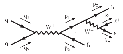
Figure 2: Feynman diagram contributing to single top production in the subdominant $s$-channel process. The top decay is also shown in this figure

The numbers quoted here correspond to total cross-sections. The separation between the sub-dominant processes and the dominant $W$-gluon fusion is purely kinematical[7, 8]. By placing a cut on the $p_{T}$ of the detected $\bar{b}$ quark, the former process can be eliminated altogether. This also eliminates a sizeable fraction of the tops produced via the $W$-gluon fusion mechanism (about two thirds for the cuts we use). The cut on $p_{T}$ has the additional bonus of making the QCD corrections manageable. One is therefore left with those single tops coming from the $W$-gluon fusion mechanism ($t$-channel) and the subdominant ${s}$-channel process. The later one is actually the main object of our interest in this article, although we will also have many comments to make on the $t$-channel process.

In a proton-proton collision a bottom-anti-top pair is also produced through analogous subprocesses. The analysis of such anti-top production processes is similar to the top ones and the corresponding cross sections can be easily derived doing the appropriate changes.

In a previous paper[8] we have analyzed the sensitivity of different LHC observables to the magnitude of the charged current effective couplings considering only the dominant $W$-gluon fusion channel. In that work we did not consider the subsequent decay of the top in any detail. We did, however, a complete analytical calculation of the subprocess cross sections, for general left and right effective couplings and including bottom mass corrections. A $p_{T}>30$ GeV cut in the transverse momentum of the produced $\bar{b}$ quark was implemented in [8] and, accordingly, only the so-called $2\rightarrow 3$ process was retained, excluding top production off a $b$-quark from the proton Fermi sea. Given the (presumed) smallness of the right handed couplings, the bottom mass plays a role which is more important than anticipated, as the mixed crossed $g_{L}g_{R}$ term, which actually is the most sensitive one to $g_{R}$, is accompanied by a $b$ quark mass. The reader is encouraged to see [8], where a very detailed analysis is presented.

Typically the top quark decays weakly well before strong interactions become relevant, so we could in principle ‘measure’ its polarization state with virtually no contamination of strong interactions (see e.g. [9, 10] for discussions this point) and try to establish interesting observables based on this measurement. In fact it is not difficult to convince oneself that in order to disentangle left from right effective couplings, it is almost compulsory to be able to ‘measure’ the polarization of the top. This will become apparent from the formulae presented in section 2. For this reason we have derived in this work and in[8] analytical expressions for the cross sections for the production of polarized tops or anti-tops. To this end one introduces the spin projector

$$\left(\frac{1+\gamma_{5}\not{n}}{2}\right),$$

with

$$n^{\mu}=\frac{1}{\sqrt{\left(p_{1}^{0}\right)^{2}-\left(\vec{p}_{1}\cdot\hat{n}\right)^{2}}}\left(\vec{p}_{1}\cdot\hat{n},p_{1}^{0}\hat{n}\right),\qquad\hat{n}^{2}=1,\qquad n^{2}=-1,$$ (2)

as the polarization projector for a particle or anti-particle of momentum $p_{1}$ with spin in the $\hat{n}$ direction. The calculation of the subprocess cross sections have been performed in this work and in [8] for an arbitrary polarization vector $\hat{n}$.

Obviously, however, the top decays very shortly after production, so the only practical way one can measure the spin of the top is through its influence on the angular distribution of the leptons produced in the decay. It is tacitly assumed in most of the works published on this subject that the decaying top is in a pure spin state for all practical purposes; i.e. its polarization vector is pointing in a particular direction in space in a given reference frame.

In the tree-level Standard Model this is not quite true, but it is almost true. The tree level Standard Model corresponds in our notation to taking $g_{L}=1$ and $g_{R}=0$. Imposing the a cut on $p_{T}$ we have mentioned, only two subprocesses contribute; $W$-gluon fusion and the $s$-channel process. The later provides 100% polarized tops in a certain direction (to be discussed latter). The situation in the $t$-channel process is a bit more complicated. The results from our previous analysis presented in [8] show that single top production is highly, but not fully, polarized in this case too (84 % in the optimal basis, with the present set of cuts). This is a high degree of polarization, but still well below the 90+ claimed by Mahlon and Parke in [10]. We understand this being due to the presence of a 30 GeV cut in $p_{T}$. In fact, if we remove this cut completely we get 91 % polarization, in rough agreement with [10] (note that we do not include the $2\rightarrow 2$ or $b$-sea process). Inasmuch as they can be compared our results for the tree-level Standard Model are in good agreement with those presented in [7] in what concerns the total cross-section. These considerations are quite independent of the choice of the strong subtraction scale, which is by far the largest source of uncertainty. Let us assume now for the sake of discussion that the polarization is indeed 100% . The top subsequently decays (say emitting a positively charged lepton). One can compute the angular probability distribution of the lepton with respect to the polarization direction in the Standard Model, multiply the two probabilities and compare the experimental result with the theoretical prediction.

In fact things are a lot more subtle. First of all, we have seen that even in the Standard Model polarization is never 100% . Furthermore, it turns out that when $g_{R}\neq 0$, i.e. beyond the Standard Model, the top can never be 100% polarized (see the discussion in section 2 and in [8]), not even in principle. In other words, the top is necessarily in a quantum mixed state and is described by a density matrix. The entries of this density matrix depend on the momenta of the incoming and outgoing particles; that is to say, there is an entanglement between spin and momenta.

Of course this complication amounts to a small effect because $g_{R}$ is surely quite small, even in most models beyond the Standard Model, so in first approximation the experimental consequences should be small. However, if our purpose is precisely to measure $g_{R}$ or at least to set a bound on it, it is clear that the effect needs to be taken into account. As already emphasized, to be able to tell left from right effective couplings one absolutely needs to consider the spin of the top.

The next step is to select the direction where one is to ‘measure’ the spin of the top. By tracing the appropriate spin operator with the density matrix one would determine the expected probabilities of finding a top that (after the measure) would point in the given direction of our choice. There is a privileged spin basis, namely the one where the density matrix is diagonal, where the calculation is greatly simplified since one needs not compute the off-diagonal terms. This diagonalization process has to be done event by event and it selects a particular vector $\hat{n}$ (event dependent). In section 5 we provide explicit formulae for this privileged direction. Elementary Quantum Mechanical considerations show that this is also the direction where the differential cross section is maximal (or minimal depending on the sign of the spin). Using this 3-vector as spin basis, for instance, one can multiply the probability of producing a top polarized in the positive $+\hat{n}$ direction with the corresponding decay angular probability distribution plus the probability of producing a top polarized in the negative $-\hat{n}$ distribution times the the corresponding decay angular probability distribution. The dependence on the effective left and right couplings $g_{L}$ and $g_{R}$ is obviously contained in the density matrix and also in the decay distributions.

Obviously, since the entries of the density matrix depend on the spin basis, the final physically observable result of the previous analysis will certainly depend on the spin basis too. How is this possible? In fact this is as it should be; we are multiplying probabilities and in fact we are neglecting the quantum interference terms because we are assuming that the polarization of the top is measured in the intermediate state before the top quark decays. Then there should be no surprise in that the interaction between the top and the apparatus measuring its spin modifies the final physical results.

However, a proper measure of the top spin before it decays is impossible; the only way we learn about top polarization is precisely from the final decay products. So, the previous procedure it is conceptually incorrect. The final result has to be strictly independent of the intermediate spin basis one uses. Does this mean that the usual procedure —which is the one we just described— is totally flawed? In principle yes, however one expects that the coarsening involved in the measuring process washes some or all of the interference effects. Then perhaps the previous procedure where one assumes that the spin of the top is well defined and one proceeds as if it could be measured before it decays it could be approximately correct. But what are then the errors involved? Do they jeopardize the determination of some of the effective couplings, in particular the distinction between $g_{L}$ and $g_{R}$? These are some of the issues we would like to address in the present work.

2 The differential cross section for polarized top production

We shall discuss here the $t$-channel production for the sake of definiteness. This is the most involved process. We refer the reader to [8] for detailed expressions of the different amplitudes. We denote the matrix elements of the hard subprocess of Fig. 1 by $M_{+}^{d}$. There will also be a $M_{+}^{\bar{u}}$, corresponding to having instead a $\bar{u}$ as spectator quark. We will also eventually define the matrix elements corresponding to the processes producing anti-tops as $M_{-}^{u}$, and $M_{-}^{\bar{d}}$. With these definitions the differential cross section for polarized tops $d\sigma$ can be written schematically as

$$d\sigma=\beta\left(f_{u}\left|M_{+}^{d}\right|^{2}+f_{\bar{d}}\left|M_{+}^{\bar{u}}\right|^{2}\right),$$

where $f_{u}$ and $f_{\bar{d}}$ denote the parton distribution functions corresponding to extracting a $u$-type quark and a $\bar{d}$-type quark respectively and $\beta$ is a proportionality factor incorporating the kinematics and also the gluon distribution function. Using our analytical results for the matrix elements given in the appendix of [8] we obtain for the differential cross-section

$$d\sigma = \beta f_{u}\left[\left|g_{L}\right|^{2}\left(a+a_{n}\right)+\left|g_{R}\right|^{2}\left(b+b_{n}\right)+\frac{g_{R}^{\ast}g_{L}+g_{R}g_{L}^{\ast}}{2}\left(c+c_{n}\right)+i\frac{g_{L}^{\ast}g_{R}-g_{R}^{\ast}g_{L}}{2}d_{n}\right]$$ (6)

$$+ \beta f_{\bar{d}}\left[\left|g_{R}\right|^{2}\left(a-a_{n}\right)+\left|g_{L}\right|^{2}\left(b-b_{n}\right)+\frac{g_{R}^{\ast}g_{L}+g_{R}g_{L}^{\ast}}{2}\left(c-c_{n}\right)-i\frac{g_{L}^{\ast}g_{R}-g_{R}^{\ast}g_{L}}{2}d_{n}\right]$$

$$= \left(\begin{array}[]{cc}g_{L}^{\ast}&g_{R}^{\ast}\end{array}\right)A\left(\begin{array}[]{c}g_{L}\\ g_{R}\end{array}\right),$$

where

$$A=\beta\left(\begin{array}[]{cc}f_{u}\left(a+a_{n}\right)+f_{\bar{d}}\left(b-b_{n}\right)&\frac{1}{2}f_{u}\left(c+c_{n}+id_{n}\right)+\frac{1}{2}f_{\bar{d}}\left(c-c_{n}-id_{n}\right)\\ \frac{1}{2}f_{u}\left(c+c_{n}-id_{n}\right)+\frac{1}{2}f_{\bar{d}}\left(c-c_{n}+id_{n}\right)&f_{u}\left(b+b_{n}\right)+f_{\bar{d}}\left(a-a_{n}\right)\end{array}\right),$$ (7)

and where $a,$ $b$, $c$, $a_{n}$, $b_{n}$, $c_{n}$ and $d_{n}$ are independent of the effective couplings $g_{R}$ and $g_{L}$ and the subscripts $n$ indicate linear dependence on the top spin four-vector $n$. All these quantities depend only on masses and momenta. The $c$, $c_{n}$ and $d_{n}$ terms are proportional to the bottom mass and are therefore absent if one neglects $m_{b}$ (this at first sight does not look unreasonable, given the energies involved). Inspection of the above differential cross-section reveals that in the $m_{b}$ limit, the only way to tell left from right effective couplings is precisely by considering and measuring polarized cross sections (the terms in $a_{n}$, $b_{n}$) unless one is willing to rely strongly on the parton distribution functions. For these reasons, both polarization and $m_{b}$ terms are quite important.

We observe that $A$ is an Hermitian matrix and therefore it is diagonalizable with real eigenvalues. Moreover, from the positivity of $d\sigma$ we immediately arrive at the constraints

$$\det A \geq 0,$$ (8)

$$TrA \geq 0,$$ (9)

that is

$$\left(f_{u}\left(a+a_{n}\right)+f_{\bar{d}}\left(b-b_{n}\right)\right)\left(f_{u}\left(b+b_{n}\right)+f_{\bar{d}}\left(a-a_{n}\right)\right)$$ (10)

$$\geq \frac{1}{4}\left(c^{2}\left(f_{u}+f_{\bar{d}}\right)^{2}+\left(c_{n}^{2}+d_{n}^{2}\right)\left(f_{u}-f_{\bar{d}}\right)^{2}+2cc_{n}\left(f_{u}^{2}-f_{\bar{d}}^{2}\right)\right),$$

and

$$\left(f_{u}+f_{\bar{d}}\right)\left(a+b\right)+\left(f_{u}-f_{\bar{d}}\right)\left(a_{n}+b_{n}\right)\geq 0.$$ (11)

Note that it is not possible to saturate both constraints for the same configuration because this would imply a vanishing $A$ which in turn would imply relations such as

$$\frac{a+b}{a_{n}+b_{n}}=\frac{f_{\bar{d}}-f_{u}}{f_{\bar{d}}+f_{u}}=\frac{a_{n}-b_{n}}{a-b},$$

which evidently do not hold. Moreover, since constraints (10) and (11) must be satisfied for any set of positive parton distribution functions we immediately obtain the bounds

$$ab+a_{n}b_{n}-\frac{1}{4}\left(c^{2}+c_{n}^{2}+d_{n}^{2}\right) \geq \left|a_{n}b+ab_{n}-\frac{1}{2}cc_{n}\right|$$

$$b^{2}+a^{2}-\left(b_{n}^{2}+a_{n}^{2}\right) \geq \frac{1}{2}\left(c^{2}-\left(c_{n}^{2}+d_{n}^{2}\right)\right).$$

In order to have a 100% polarized top we need a spin four-vector $n$ that saturates the constraint (8) (that is Eq.(10)) for each kinematical situation, that is we need $A\left(n\right)$ to have a zero eigenvalue which is equivalent to have a unitary matrix $C$ satisfying

$$C^{\dagger}AC=\mathrm{diag}\left(\lambda,0\right),$$

for some positive eigenvalue $\lambda$. In general such $n$ need not exist and, should it exist, is in any case independent of the effective couplings $g_{R}$ and $g_{L}$. Moreover, provided this $n$ exists there is only one solution (up to a global complex normalization factor $\alpha$) for the pair $\left(g_{R},g_{L}\right)$ to the equation $d\sigma=0,$ This solution is just

$$g_{L} = \alpha C_{12},$$

$$g_{R} = \alpha C_{22}.$$ (12)

Note that if one of the effective couplings vanishes we can take the other constant and arbitrary. However if both effective couplings are non-vanishing we would have a quotient $g_{R}/g_{L}$ that would depend in general on the kinematics. This is not possible so we can conclude that for a non-vanishing $g_{R}$ ( $g_{L}$ is evidently non-vanishing) it is not possible to have a pure spin state (or, else, only for fine tuned $g_{R}$ a 100% polarization is possible).

Let us now give a very simple example to make the previous discussion more understandable: in the un-physical situation where $m_{t}\rightarrow 0$ it can be shown that there exists two solutions to the saturated constraint (8), namely

$$m_{t}n^{\mu}\rightarrow\pm\left(\left|\vec{p}_{1}\right|,p_{1}^{0}\frac{\vec{p}_{1}}{\left|\vec{p}_{1}\right|}\right),$$ (13)

once we have found this result we plug it in the expression (12) and we find the solutions $\left(0,g_{L}\right)$ with $g_{L}$ arbitrary for the $+$ sign and $\left(g_{R},0\right)$ with $g_{R}$ arbitrary for the $-$ sign. That is, physically we have zero probability of producing a right handed top when we have only a left handed coupling and viceversa when we have only a right handed coupling. Note that in this case it is clear that having both effective couplings non-vanishing would imply the absence of 100 % polarization in any spin basis. This can be understood in general remembering that the top particle forms in general an entangled state with the other particles of the process. Since we are tracing over the unknown spin degrees of freedom and over the flavors of the spectator quark we do not end up with a top in a pure polarized state.

3 Cross-sections for top production and decay in the $s$-channel

Let us now turn to the $s$-channel process. This is, as already mentioned, subdominant but non-negligible since it roughly amounts to a 10% of all single tops produced after our set of cuts are imposed. It is also a lot cleaner from a theoretical point of view, as QCD corrections are small. As a by-product we shall derive the differential decay width, which is applicable to both the $t$ and $s$-channel processes.

Using the momenta conventions of Fig. 2 and averaging over colors and spins of the initial fermions and summing over colors and spins of the final fermions (remember that we have included a spin projector for the top) the squared amplitude for top production is given by

$$\left|M_{n}\right|^{2} = \frac{e^{4}N_{c}}{s_{W}^{4}}\left(\frac{1}{k^{2}-M_{W}^{2}}\right)^{2}$$ (14)

$$\times\left\{\left|\tilde{g}_{L}\right|^{2}\left[\left|g_{R}\right|^{2}\left(q_{1}\cdot\frac{p_{1}+m_{t}n}{2}\right)\left(q_{2}\cdot\tilde{p}_{2}\right)+\left|g_{L}\right|^{2}\left(q_{2}\cdot\frac{p_{1}-m_{t}n}{2}\right)\left(q_{1}\cdot\tilde{p}_{2}\right)\right.\right.$$

$$+m_{b}\frac{g_{L}g_{R}^{\ast}+g_{R}g_{L}^{\ast}}{4}\left[m_{t}\left(q_{1}\cdot q_{2}\right)+\left(q_{2}\cdot p_{1}\right)\left(q_{1}\cdot n\right)-\left(q_{2}\cdot n\right)\left(q_{1}\cdot p_{1}\right)\right]$$

$$+\left.\left.im_{b}\frac{g_{L}g_{R}^{\ast}-g_{R}g_{L}^{\ast}}{4}\varepsilon_{\mu\alpha\rho\sigma}n^{\mu}p_{1}^{\alpha}q_{1}^{\rho}q_{2}^{\sigma}\right]\right\}$$

$$+\left|\tilde{g}_{R}\right|^{2}\left[\left|g_{R}\right|^{2}\left(q_{2}\cdot\frac{p_{1}+m_{t}n}{2}\right)\left(q_{1}\cdot\tilde{p}_{2}\right)+\left|g_{L}\right|^{2}\left(q_{1}\cdot\frac{p_{1}-m_{t}n}{2}\right)\left(q_{2}\cdot\tilde{p}_{2}\right)\right.$$

$$+m_{b}\frac{g_{L}g_{R}^{\ast}+g_{R}g_{L}^{\ast}}{4}\left[m_{t}\left(q_{1}\cdot q_{2}\right)+\left(q_{1}\cdot p_{1}\right)\left(q_{2}\cdot n\right)-\left(q_{1}\cdot n\right)\left(q_{2}\cdot p_{1}\right)\right]$$

$$+\left.\left.im_{b}\frac{g_{L}g_{R}^{\ast}-g_{R}g_{L}^{\ast}}{4}\varepsilon_{\mu\alpha\rho\sigma}n^{\mu}p_{1}^{\alpha}q_{2}^{\rho}q_{1}^{\sigma}\right]\right\},$$

where $\tilde{g}_{L},$ and $\tilde{g}_{R}$ are left and right couplings to light quarks and $g_{L}$ and $g_{R}$ are the effective couplings to the top- bottom system. In the numerical results we have taken $\tilde{g}_{L}=1,$ $\tilde{g}_{R}=0$; i.e. we stick to the tree-level Standard Model values in the light sector, but is quite straightforward to include more general couplings. Notice that, exactly as for the $t$-channel, the crossed $g_{L}g_{R}$ terms vanish in the differential cross-section in the $m_{b}\to 0$ limit. Also for exactly the same reasons as in the $t$-channel analysis, modulo parton distribution functions effects, the differential unpolarized production cross section would be proportional to $|g_{L}|^{2}+|g_{R}|^{2}$.

The differential cross section for producing polarized tops is then

$$d\sigma_{\hat{n}} = f\left(\tilde{x}_{1},\tilde{x}_{2},\left(q_{1}+q_{2}\right)^{2},\Lambda_{QCD}\right)d\tilde{x}_{1}d\tilde{x}_{2}\frac{1}{4\left|q_{2}^{0}\overrightarrow{q_{1}}-\overrightarrow{q_{2}}q_{1}^{0}\right|}$$

$$\times\frac{d^{3}p_{1}}{\left(2\pi\right)^{3}2p_{1}^{0}}\frac{d^{3}\tilde{p}_{2}}{\left(2\pi\right)^{3}2\tilde{p}_{2}^{0}}\left|M_{n}\right|^{2}\left(2\pi\right)^{4}\delta^{4}\left(q_{1}+q_{2}-p_{1}-p_{2}\right)$$

where $f\left(\tilde{x}_{1},\tilde{x}_{2},\left(q_{1}+q_{2}\right)^{2},\Lambda_{QCD}\right)d\tilde{x}_{1}d\tilde{x}_{2}$ accounts for the quarks parton distribution functions.

The total decay rate of the top, on the other hand, with arbitrary left and right effective couplings is given by

$$\Gamma = \frac{e^{2}}{s_{W}^{2}}\left\{\left(\left|g_{L}\right|^{2}+\left|g_{R}\right|^{2}\right)\left(m_{t}^{2}+m_{b}^{2}-2M_{W}^{2}+\frac{\left(m_{t}^{2}-m_{b}^{2}\right)^{2}}{M_{W}^{2}}\right)\right.$$

$$\left.-12m_{t}m_{b}\frac{g_{L}g_{R}^{\ast}+g_{R}g_{L}^{\ast}}{2}\right\}\frac{\sqrt{\left(m_{t}^{2}+m_{b}^{2}-M_{W}^{2}\right)^{2}-4m_{t}^{2}m_{b}^{2}}}{64\pi m_{t}^{2}p_{1}^{0}}.$$

The squared amplitude corresponding to the decay rate in the channel depicted in Fig. (2) summing over the top polarizations (with a spin projector inserted), averaging over its color and summing over colors and polarizations of decay products is given by

$$\left|M_{n}^{D}\right|^{2}=-\frac{4}{N_{c}}\left|M_{n}\right|^{2}\left(q_{1}\rightarrow k_{2},\ q_{2}\rightarrow k_{1},\ \tilde{p}_{2}\rightarrow-p_{2}\right),$$ (15)

where $\left|M_{n}\right|^{2}\left(q_{1}\rightarrow k_{2},\ q_{2}\rightarrow k_{1},\ \tilde{p}_{2}\rightarrow-p_{2}\right)$ is just expression (14) with the indicated changes in momenta. In the above expression $\tilde{g}_{L},$ and $\tilde{g}_{R}$ are the left and right couplings corresponding to the lepton-neutrino vertex. We have assumed $\tilde{g}_{L}=1,$ $\tilde{g}_{R}=0$, but again this hypothesis can be relaxed. The decay rate differential distribution for this channel is given by

$$d\Gamma_{n}=\frac{\left|M_{n}^{D}\right|^{2}}{2p_{1}^{0}}\frac{d^{3}k_{1}}{\left(2\pi\right)^{3}2k_{2}^{0}}\frac{d^{3}k_{2}}{\left(2\pi\right)^{3}2k_{1}^{0}}\frac{d^{3}p_{2}}{\left(2\pi\right)^{3}2p_{2}^{0}}\left(2\pi\right)^{4}\delta^{4}\left(k_{1}+k_{2}+p_{2}-p_{1}\right).$$

Finally, using the narrow-width approximation, we have that the differential cross section $d\sigma$ corresponding to Fig. 2 is given by

$$d\sigma=\sum_{\pm n}d\sigma_{n}\times\frac{d\Gamma_{n}}{\Gamma}.$$ (16)

4 The role of spin in the narrow-width approximation

Within the narrow-width approximation we just discussed we decompose the process depicted in Fig. 2 in two consecutive processes: the top production and its consecutive decay. In that set up we denote the single top production amplitude as $A_{p,\pm\hat{n}\left(p\right)}$ and the top decay amplitude as $B_{p,\pm\hat{n}\left(p\right)}.$ In the polar representation we write

$$A_{p,\pm\hat{n}\left(p\right)} = \left|A_{p,\pm\hat{n}\left(p\right)}\right|e^{i\varphi_{\pm}\left(p\right)},$$

$$B_{p,\pm\hat{n}\left(p\right)} = \left|B_{p,\pm\hat{n}\left(p\right)}\right|e^{i\omega_{\pm}\left(p\right)},$$

where $p$ indicate external momenta and $\hat{n}\left(p\right)$ a given spin basis for the top. The differential cross section for the whole process is schematically given by

$$d\mathcal{\sigma}=\int\left|A_{p,+\hat{n}\left(p\right)}B_{p,+\hat{n}\left(p\right)}+A_{p,-\hat{n}\left(p\right)}B_{p,-\hat{n}\left(p\right)}\right|^{2}dp.$$ (17)

Hence

$$d\mathcal{\sigma} = \int\left|A_{p,+\hat{n}\left(p\right)}\right|^{2}\left|B_{p,+\hat{n}\left(p\right)}\right|^{2}dp+\int\left|A_{p,-\hat{n}\left(p\right)}\right|^{2}\left|B_{p,-\hat{n}\left(p\right)}\right|^{2}dp$$ (18)

$$+2\int\left|A_{p,+\hat{n}\left(p\right)}\right|\left|B_{p,+\hat{n}\left(p\right)}\right|\left|A_{p,-\hat{n}\left(p\right)}\right|\left|B_{p,-\hat{n}\left(p\right)}\right|$$

$$\times\cos\left(\varphi_{+}\left(p\right)-\varphi_{-}\left(p\right)+\omega_{+}\left(p\right)-\omega_{-}\left(p\right)\right)dp$$

$$\simeq \int\left|A_{p,+\hat{n}\left(p\right)}\right|^{2}\left|B_{p,+\hat{n}\left(p\right)}\right|^{2}dp+\int\left|A_{p,-\hat{n}\left(p\right)}\right|^{2}\left|B_{p,-\hat{n}\left(p\right)}\right|^{2}dp.$$

Since the axis with respect to which the spin basis is defined is completely arbitrary $d\mathcal{\sigma}$ is independent on this choice of basis. However within the narrow width approximation one never computes $d\mathcal{\sigma}$ following formula (17). The commonly used procedure [10, 14] consists in computing the probability of producing a polarized top and then multiplying this probability by the probability of a given decay channel (see Eq. (16)). This procedure is equivalent to the neglection of the interference term in formula (18) as indicated there. First of all, as discussed in the introduction, if one neglects the interference term, the result depends on the spin basis; i.e. on the direction one chooses to measure the third component of the top spin. This is of course acceptable if one really performs a physical measure of the spin (in the $\hat{n(p)}$ direction in this case) since the interaction with the apparatus modifies the state. A dependence on the spin frame is however unacceptable if the spin is not measured before the top decays.

Let us see whether this approximation can justified nevertheless. Clearly, the integration over momenta enhances the positive-definite terms in front of the interference oscillating one. If in addition we make a choice for $\hat{n}\left(p\right)$ that diagonalizes the top spin density matrix and thus maximizes $\left|A_{p,+\hat{n}\left(p\right)}\right|$ and minimizes $\left|A_{p,-\hat{n}\left(p\right)}\right|$, then we expect the interference term to be negligible when compared to $\int\left|A_{p,+\hat{n}\left(p\right)}\right|^{2}\left|B_{p,+\hat{n}\left(p\right)}\right|^{2}dp$ even for small amount of phase space integration. In the s-channel we will see in the next section that the limit of $g_{R}\rightarrow 0$ there exists a spin basis $\hat{n}\left(p\right)$ where $\left|A_{p,-\hat{n}\left(p\right)}\right|$ is strictly zero. This basis is given by

$$n=\frac{1}{m_{t}}\left(\frac{m_{t}^{2}}{\left(q_{2}\cdot p_{1}\right)}q_{2}-p_{1}\right).$$

From this it follows that for small $g_{R}$ if we use that basis the interference integrand is already negligible with respect to the dominant term $\int\left|A_{p,+\hat{n}\left(p\right)}\right|^{2}\left|B_{p,+\hat{n}\left(p\right)}\right|^{2}dp$. For $g_{R}\neq 0$ one can still find a basis that maximizes $\left|A_{p,+\hat{n}\left(p\right)}\right|$ (and minimizes $\left|A_{p,-\hat{n}\left(p\right)}\right|$) and therefore diagonalizes the top density matrix $\rho$. In the next section we will show how to obtain such a basis that will be the one used in our numerical integration. In these simulations we have checked numerically that this basis is the one that maximizes $d\mathcal{\sigma}$ and therefore, on the same grounds, the one that minimizes the interference term. The same considerations can be applied to the $t$-channel process.

Given that the observables are strictly independent of the choice of spin basis only if the interference term is included, we can easily assess the importance of the latter by checking to what extent a residual spin basis dependence is present. We have checked numerically this point by changing the definition of the spin basis $\hat{n}\left(p\right)$ and noting that our results are actually only weakly dependent on the choice of $\hat{n}\left(p\right)$ even for a small amount of coarsening. A 4% maximum variation in $p_{T}$ distributions was found between the optimal diagonal basis and another basis orthogonal to the beam axis (that is, almost orthogonal to all momenta). Moreover we have checked that if spin is ignored altogether (by considering unpolarized top production) roughly the same amount of variation with respect to the diagonal basis is observed. Thus we conclude that even though the dependence on the choice of spin basis is not dramatic, its consideration is a must for a precise description using the narrow-width approximation taking into account the presumed smallness of the effective coupling to be measured and how subtle the experimental distinction of left and right couplings turns out to be.

5 The diagonal basis

As stated in the previous section in order to calculate the top decay we have to find the basis where the polarized single top production cross section is maximal. The can do this maximizing in the $4$-dimensional space generated by the components of $n$ constrained by

$$n\cdot p_{1}=0,\qquad n^{2}=-1,$$ (19)

where $p_{1}$ is the top four-moment, that is

$$n^{0} = \frac{n^{1}p_{1}^{1}+n^{2}p_{1}^{2}+n^{2}p_{1}^{2}}{p_{1}^{0}},$$

$$\left(p_{1}^{0}\right)^{2} = \left(p_{1}^{0}\right)^{2}\left\|\vec{n}\right\|^{2}-\left(n^{1}p_{1}^{1}+n^{2}p_{1}^{2}+n^{2}p_{1}^{2}\right)^{2},$$

where $\left\|\vec{n}\right\|=\sqrt{\left(n^{1}\right)^{2}+\left(n^{2}\right)^{2}+\left(n^{3}\right)^{2}}$, that is $n^{i}=\left\|\vec{n}\right\|\hat{n}^{i}$ with $\hat{n}$ the normalized spin three-vector. From above equations we obtain

$$\left\|\vec{n}\right\| = \frac{p_{1}^{0}}{\sqrt{\left(p_{1}^{0}\right)^{2}-\left(\hat{n}^{1}p_{1}^{1}+\hat{n}^{2}p_{1}^{2}+\hat{n}^{2}p_{1}^{2}\right)^{2}}},$$

$$n^{0} = \left\|\vec{n}\right\|\frac{\hat{n}^{1}p_{1}^{1}+\hat{n}^{2}p_{1}^{2}+\hat{n}^{2}p_{1}^{2}}{p_{1}^{0}},$$

from which Eq. (2) follows immediately. Let us now find the polarization vector that maximizes and minimizes the differential cross section of single top production.

5.1 The t-channel

We will begin with the t-channel the was analyzed in the previous chapter. Using Eq. (6) we define

$$a_{n} = n\cdot a,\qquad b_{n}=n\cdot b,$$

$$c_{n} = n\cdot c,\qquad d_{n}=n\cdot d,$$ (20)

and using Lagrange multipliers $\lambda_{1}$ and $\lambda_{2}$ for constraints (19) we maximize

$$\sigma+\lambda_{1}\left(n^{2}+1\right)+\lambda_{2}n\cdot p_{1},$$

obtaining the equations

$$n = -\frac{\beta}{2\lambda_{1}}f_{u}\left[\left|g_{L}\right|^{2}a+\left|g_{R}\right|^{2}b+\frac{g_{R}^{\ast}g_{L}+g_{R}g_{L}^{\ast}}{2}c+i\frac{g_{L}^{\ast}g_{R}-g_{R}^{\ast}g_{L}}{2}d\right]$$ (21)

$$+\frac{\beta}{2\lambda_{1}}f_{\bar{d}}\left[\left|g_{R}\right|^{2}a+\left|g_{L}\right|^{2}b+\frac{g_{R}^{\ast}g_{L}+g_{R}g_{L}^{\ast}}{2}c+i\frac{g_{L}^{\ast}g_{R}-g_{R}^{\ast}g_{L}}{2}d\right]-\frac{\lambda_{2}}{2\lambda_{1}}p_{1},$$

$$0 = n^{2}+1,$$ (22)

$$0 = n\cdot p_{1},$$ (23)

and thus using Eqs. (21) and (23)

$$\lambda_{2} = -\frac{\beta}{m_{t}^{2}}f_{u}\left[\left|g_{L}\right|^{2}a\cdot p_{1}+\left|g_{R}\right|^{2}b\cdot p_{1}+\frac{g_{R}^{\ast}g_{L}+g_{R}g_{L}^{\ast}}{2}c\cdot p_{1}+i\frac{g_{L}^{\ast}g_{R}-g_{R}^{\ast}g_{L}}{2}d\cdot p_{1}\right]$$

$$+\frac{\beta}{m_{t}^{2}}f_{\bar{d}}\left[\left|g_{R}\right|^{2}a\cdot p_{1}+\left|g_{L}\right|^{2}b\cdot p_{1}+\frac{g_{R}^{\ast}g_{L}+g_{R}g_{L}^{\ast}}{2}c\cdot p_{1}+i\frac{g_{L}^{\ast}g_{R}-g_{R}^{\ast}g_{L}}{2}d\cdot p_{1}\right],$$

and therefore

$$n = \frac{\beta}{2\lambda_{1}}\left\{\left(f_{u}\left|g_{L}\right|^{2}-f_{\bar{d}}\left|g_{R}\right|^{2}\right)\left(\frac{a\cdot p_{1}}{m_{t}^{2}}p_{1}-a\right)+\left(f_{u}\left|g_{R}\right|^{2}-f_{\bar{d}}\left|g_{L}\right|^{2}\right)\left(\frac{b\cdot p_{1}}{m_{t}^{2}}p_{1}-b\right)\right.$$

$$+\left.\frac{g_{R}^{\ast}g_{L}+g_{R}g_{L}^{\ast}}{2}\left(f_{u}-f_{\bar{d}}\right)\left(\frac{c\cdot p_{1}}{m_{t}^{2}}p_{1}-c\right)+i\frac{g_{L}^{\ast}g_{R}-g_{R}^{\ast}g_{L}}{2}\left(f_{u}-f_{\bar{d}}\right)\left(\frac{d\cdot p_{1}}{m_{t}^{2}}p_{1}-d\right)\right\},$$

with the normalization factor $\lambda_{1}$ given by Eq. (22). Note that in the idealized case $f_{u}=f_{\bar{d}}=f$ we obtain

$$n=\alpha\left\{\frac{\left(a-b\right)\cdot p_{1}}{m_{t}^{2}}p_{1}-\left(a-b\right)\right\},$$

where $\alpha$ is the normalization constant that does not depend on $f$ or the effective couplings. In the SM ($g_{R}=0$) we obtain

$$n=\alpha\left(f_{u}\left(\frac{a\cdot p_{1}}{m_{t}^{2}}p_{1}-a\right)-f_{\bar{d}}\left(\frac{b\cdot p_{1}}{m_{t}^{2}}p_{1}-b\right)\right),$$

where $\alpha$ is a normalizing factor.

5.2 The s-channel

The s-channel differential cross section has the form

$$d\sigma = \beta\left(f_{u}f_{\bar{d}}+f_{c}f_{\bar{s}}\right)\left[\left|g_{L}\right|^{2}\left(a_{s}+a_{n}\right)+\left|g_{R}\right|^{2}\left(b_{s}+b_{n}\right)\right.$$

$$+\left.\frac{g_{R}^{\ast}g_{L}+g_{R}g_{L}^{\ast}}{2}\left(c_{s}+c_{n}\right)+i\frac{g_{L}^{\ast}g_{R}-g_{R}^{\ast}g_{L}}{2}d_{n}\right],$$

where again $\beta$ is a proportionality incorporating the kinematics, and where $f_{u,c}$ and $f_{\bar{d},\bar{s}}$ denote the parton distribution functions corresponding to extracting a $u,c$-type quarks and a $\bar{d},\bar{s}$-type quarks respectively. Using again the decomposition (20) and proceeding analogously to the t-channel calculation we obtain

$$n = \alpha\left\{\left|g_{L}\right|^{2}\left(\frac{a\cdot p_{1}}{m_{t}^{2}}p_{1}-a\right)+\left|g_{R}\right|^{2}\left(\frac{b\cdot p_{1}}{m_{t}^{2}}p_{1}-b\right)\right.$$ (24)

$$+\left.\frac{g_{R}^{\ast}g_{L}+g_{R}g_{L}^{\ast}}{2}\left(\frac{c\cdot p_{1}}{m_{t}^{2}}p_{1}-c\right)+i\frac{g_{L}^{\ast}g_{R}-g_{R}^{\ast}g_{L}}{2}\left(\frac{d\cdot p_{1}}{m_{t}^{2}}p_{1}-d\right)\right\},$$

where $\alpha$ is the normalizing factor that in this case (unlike in the t-channel result) does not depend on the parton distribution functions. From Eq. (14) we obtain

$$a^{\mu} = -m_{t}q_{2}^{\mu}\left(q_{1}\cdot\tilde{p}_{2}\right),$$

$$b^{\mu} = +m_{t}q_{1}^{\mu}\left(q_{2}\cdot\tilde{p}_{2}\right),$$

$$c^{\mu} = +m_{b}\left(q_{1}^{\mu}\left(q_{2}\cdot p_{1}\right)-q_{2}^{\mu}\left(q_{1}\cdot p_{1}\right)\right),$$

$$d^{\mu} = -m_{b}\varepsilon_{~{}\alpha\rho\sigma}^{\mu}p_{1}^{\alpha}q_{1}^{\rho}q_{2}^{\sigma},$$

hence replacing in Eq. (24) we arrive at

$$n^{\mu} = \alpha\left\{\left|g_{L}\right|^{2}\left(\left(q_{1}\cdot\tilde{p}_{2}\right)\left(q_{2}\cdot p_{1}\right)p_{1}^{\mu}-\left(q_{1}\cdot\tilde{p}_{2}\right)m_{t}^{2}q_{2}^{\mu}\right)\right.$$ (25)

$$+\left|g_{R}\right|^{2}\left(\left(q_{2}\cdot\tilde{p}_{2}\right)\left(q_{1}\cdot p_{1}\right)p_{1}^{\mu}-\left(q_{2}\cdot\tilde{p}_{2}\right)m_{t}^{2}q_{1}^{\mu}\right)$$

$$+m_{b}m_{t}\frac{g_{R}^{\ast}g_{L}+g_{R}g_{L}^{\ast}}{2}\left(q_{1}^{\mu}\left(q_{2}\cdot p_{1}\right)-q_{2}^{\mu}\left(q_{1}\cdot p_{1}\right)\right)$$

$$+\left.i\frac{g_{R}^{\ast}g_{L}-g_{L}^{\ast}g_{R}}{2}m_{b}m_{t}\varepsilon_{~{}~{}\alpha\rho\sigma}^{\mu}p_{1}^{\alpha}q_{1}^{\rho}q_{2}^{\sigma}\right\},$$

which is the basis we use in our numerical simulations. If we neglect $g_{R}$ we obtain

$$n^{\mu}=\pm\frac{\left(q_{1}\cdot\tilde{p}_{2}\right)\left(q_{2}\cdot p_{1}\right)p_{1}^{\mu}-\left(q_{1}\cdot\tilde{p}_{2}\right)m_{t}^{2}q_{2}^{\mu}}{\sqrt{\left(q_{1}\cdot\tilde{p}_{2}\right)^{2}\left(q_{2}\cdot p_{1}\right)^{2}m_{t}^{2}-\left(q_{1}\cdot\tilde{p}_{2}\right)^{2}m_{t}^{4}q_{2}^{2}}},$$

where we have included the normalization factor and since $q_{2}^{2}=0$ the above reduces to

$$m_{t}n=\pm\left(\frac{m_{t}^{2}}{\left(q_{2}\cdot p_{1}\right)}q_{2}-p_{1}\right),$$

which is the result we have quoted in the previous section coinciding with [10]

6 Numerical analysis of $s$-channel single top production

Let us start this section by discussing the experimental cuts we have implemented. Due to geometrical detector constraints[15] we cut off very low angles for the outgoing particles. The charged particles in the final state have to come out with an angle in between 10 and 170 degrees to be detected. These angular cuts correspond to a cut in pseudorapidity $\left|\eta\right|<2.44$. In order to be able to separate the jets corresponding to the outgoing particles we implement isolation cuts of 20 degrees between each other. These are the appropriate cuts for general purpose experiments such as ATLAS or CMS.

The set of cuts used in this work are compatible with the ones used in the t-channel. Since in the previous paper [8] top decay was not considered, the equivalence is only approximate and a more detailed phenomenological analysis will be required in due course (it is actually quite straightforward with the help of the results presented here to redo the $t$-channel study, but this goes beyond the scope of this paper). The present analysis should however suffice in any case to identify the most promising observables and get a rough estimate of the precision that it can be reached.

We use a lower cut of 20 GeV in the $\bar{b}$ jet. This completely eliminates top production from a $b$-quark from the proton sea and greatly reduces higher order QCD contributions. In the $t$-channel reduces the cross section to about one third of its total value, since typically the $\bar{b}$ quark comes out in the same direction as the incoming gluon and a large fraction of them do not pass the cut. Similarly, $p_{T}>20$ GeV cuts are set for the top and spectator quark jets. These cuts guarantee the validity of perturbation theory and will serve to separate from the overwhelming background of low $p_{T}$ physics. These values come as a compromise to preserve a good signal, while suppressing unwanted contributions. They are very similar to the ones used in [7] and [10].

In order to calculate the cross section $\sigma$ of the process $pp\rightarrow t\bar{b}$ we have used the CTEQ4 set of structure functions [17] to determine the probability of extracting a parton with a given fraction of momenta from the proton. To calculate the total event production corresponding to different observables we have used the integrating Monte Carlo program VEGAS [18]. We present results after one year (defined as 10⁷ seg.) run at full luminosity in one detector (100 $\mathrm{fb}^{-1}$ at LHC).

Since in order to be able to perform the effective $Wt\bar{b}$ coupling one definitely needs to tag the two $b$-type quarks, this value for the luminosity is surely too high. The $b$ physics program at ATLAS [19], for instance, it is planned to be done at one tenth of the total luminosity to avoid pile-up effects. This is even more so in a dedicated detector such as LHCb[16] where the appropriate figure is expected to be 2 fb^-1. ATLAS plans to do most of the $b$-physics runs before full luminosity is reached, for instance. We have nonetheless used the high luminosity figure since at this stage the experimental strategy is not totally settled yet.

The way we proceed is the following. We analyze the kinematics of each event including a $\bar{b}$ that passes the experimental cuts and reconstruct the vector $\hat{n}$ using the analytic formulae presented in the previous sections. As the reader will remember, this provides us with a spin basis that minimizes the quantum interference terms. We then proceed to multiply the probabilities classically —just as if we pretend that the top spin has been measured in the direction determined by $\hat{n}$ and we determine the decay probability distribution. We retain only those final states that pass the remaining cuts.

In the same way and choosing arbitrary spin directions we are able to see how much the physical results depend on the interference term. We have found a 4% difference between the worst case (a spin direction perpendicular to almost all 3-momenta involved) and the optimal case (found analytically here). We have every reason to believe that, after the integration over momenta and the resulting coarsening, the interference term is in this basis all but negligible. The rest of the results presented in this section are all worked out in the optimal spin basis.

Let us first review the results obtained in the framework of the tree-level standard model. This corresponds to taking $g_{L}=1$ and $g_{R}=0$ in all our formulae. The results are summarized in Figs. 3, 4, 5. The first of these figures show how the final products of the process are predominantly emitted in the axis direction (albeit not so much as in the case of the $t$-channel production) and in the same direction. The plot shows the direction respect to the beam of bottom and anti-bottom. Recall that a 10 degree cut is implemented, as well as a separation cut of 20 degrees among all jets. Fig. 4 shows the $p_{T}$ distribution for the $\bar{b}$, showing the 20 GeV cut on the $p_{T}$ of the $\bar{b}$ enforced.

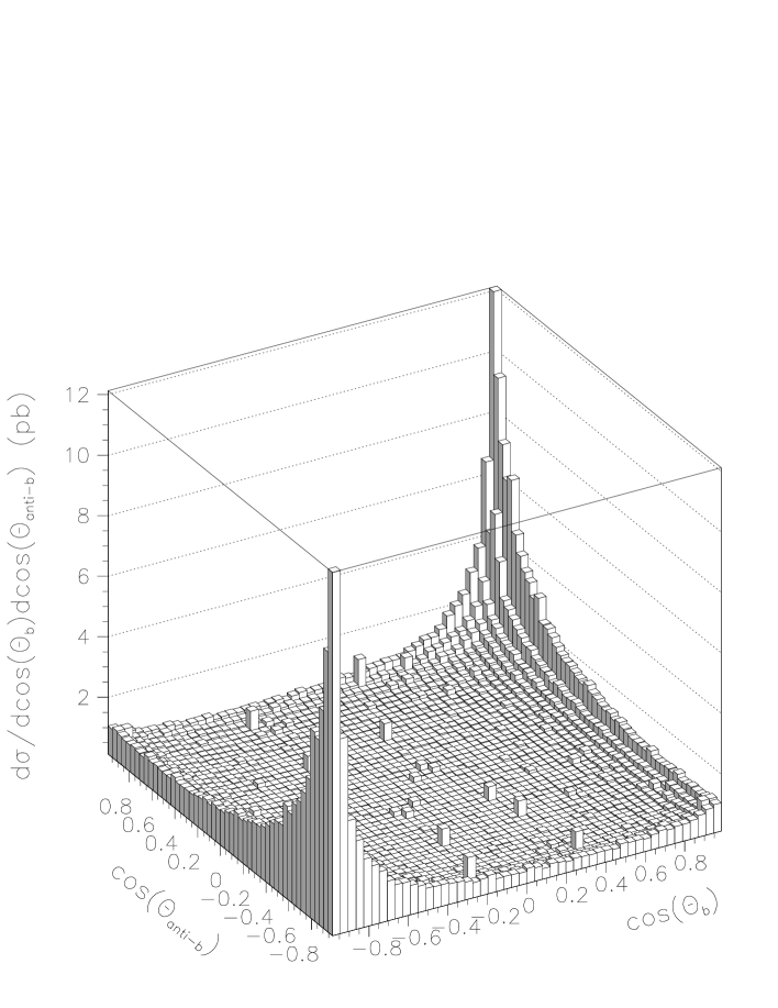
Figure 3: Distribution of the cosines of the polar angles of the bottom and anti-bottom with respect to the beam line. The plot corresponds to single top production at the LHC with top decay included. The calculation was performed at the tree level in Standard Model. For the parton distribution functions we use $\mu^{2}=\hat{s}=\left(q_{1}+q_{2}\right)^{2}$.

Figure 4: Anti-bottom transversal momentum distribution corresponding to single top production at the LHC. The calculation has been performed at tree level in the SM ($g_{L}=1$, $g_{R}=0$).

Figure 5: Distribution of the invariant mass of the lepton (electron or muon) plus bottom system arising in top decay from single top production at the LHC. The calculation was performed at the tree level in Standard Model with $\mu^{2}=\hat{s}=\left(q_{1}+q_{2}\right)^{2}$.

Fig. 5 shows the invariant mass of the lepton and bottom system in the tree level Standard Model. Since we are working in the narrow width approximation, the distribution falls to zero just below the physical mass of the top and this reflects the part of the total momentum of the top carried away by the undetected neutrino. Figs. 6 and 7 actually show the $p_{T}$ distribution for the bottom and lepton, respectively, that are produced in the top decay. As previously discussed, 20 GeV cuts on the respective $p_{T}$ are imposed. Even though some information is lost by the fact that the neutrino is not seen and therefore there is some amount of missing momentum, this does not seem to affect the sensitivity to the effective couplings too much. One could as well consider channels in which the $W^{+}$, produced in the top decay, decays hadronically. In hadronic decays of the top a full reconstruction of the top mass would be feasible.

Figure 6: Bottom transversal momentum distribution corresponding to single top production at the LHC. The calculation has been performed at tree level in the SM ($g_{L}=1$, $g_{R}=0$).

Figure 7: Lepton (electron or muon) transversal momentum distribution corresponding to single top production at the LHC. The calculation has been performed at tree level in the SM ($g_{L}=1$, $g_{R}=0$).

Let us now move beyond the Standard Model. Since changing the value of $g_{L}$ (while keeping $g_{R}=0$) amounts to a simple rescaling, we shall concentrate on the more interesting case of varying $g_{R}$. As a rough order-of-magnitude estimate for the effective $g_{R}$ coupling we take $|g_{R}|=5\times 10^{-2}$. This is still worse than the limit implied by $b\to s\gamma$, but is the sort of sensitivity that LHC will be able to set. The effects are linear in $g_{R}$, so it is easy to scale up or down the results. We have consider the possibility of $g_{R}$ having a phase and, accordingly, the experimental sensitivity to that phase.

We have found that the anti-lepton plus bottom invariant mass distribution we just discussed in the previous paragraph is actually sensitive to $g_{R}$. Figs. 8 and 9 reflect this sensitivity with the second figure showing the statistical significance per bin.

Figure 8: Event production difference between non-vanishing $g_{R}$ coupling caculations and the tree level SM ones ($g_{R}=0$). Differences are plotted versus the invariant mass of the lepton (electron or muon) plus bottom system arising in top decay from single top production at the LHC. We have taken $g_{R}=+5\times 10^{-2}$, $+i5\times 10^{-2},$ $-5\times 10^{-2}$ and $-i5\times 10^{-2}$ in plots (a), (b), (c) and (d) respectively. With the present set of cuts, the total number of events in the Standard Model is 181,000. The total excess is 1,200, roughly 1% .

Figure 9: Plots corresponding to differences (a), (b) (c) and (d) of Fig. (8) divided by the square root of the event production per bin at LHC. The square of the quotient denominator can be obtained from Fig. (5) multiplying $d\sigma/dm_{inv}$ by the LHC 1-year full luminosity (100 $\mathrm{fb}^{-1}$) and by the width of each bin (4 GeV. in Fig. (5)). Taking the modulus of the above plots we obtain the statistical significance of the corresponding signals per bin. Note that statistical significance has a strong and non-linear dependence both on the invariant mass and the right coupling $g_{R.}$ However purely imaginary couplings are almost insensible to their sign.

We shall now show the dependence of the three $p_{T}$ distributions ($b$, $\bar{b}$ and lepton) to the modulus and phase of the effective coupling $g_{R}$. In all cases the value $g_{L}=1$ is taken. The sensitivity to departures from the tree level SM is shown in Figs. (10), (11) and (12).

Figure 10: Statistical significance per bin with respect to anti-bottom transversal momentum. Like in Fig. (9) we have taken $g_{R}=+5\times 10^{-2}$, $+i5\times 10^{-2},$ $-5\times 10^{-2}$ and $-i5\times 10^{-2}$ in plots (a), (b), (c) and (d) respectively. Note that here statistical significance has a strong dependence on the anti-bottom transversal momentum but is almost linear on $\emph{Re}\left(g_{R}\right)$ and almost insensible to the sign of $\emph{Im}\left(g_{R}\right)$.

Figure 11: Like in Fig. (9) we have taken $g_{R}=+5\times 10^{-2}$, $+i5\times 10^{-2},$ $-5\times 10^{-2}$ and $-i5\times 10^{-2}$ in plots (a), (b), (c) and (d) respectively. Note that here statistical significance has a strong dependence on the bottom transversal momentum and clearly favors positive values of $\emph{Re}\left(g_{R}\right)$ and again is insensible to the sign of $\emph{Im}\left(g_{R}\right)$.

Figure 12: Statistical significance of the corresponding signals per bin with respect to lepton (electron or muon) transversal momentum. Like in Fig. (9) we have taken $g_{R}=+5\times 10^{-2}$, $+i5\times 10^{-2},$ $-5\times 10^{-2}$ and $-i5\times 10^{-2}$ in plots (a), (b), (c) and (d) respectively. Note that again statistical significance has a strong dependence on the lepton transversal momentum and clearly favors positive values of $\emph{Re}\left(g_{R}\right).$ The sign of $\emph{Im}\left(g_{R}\right)$ cannot be distinguished.

We also include the statistical significance per bin for the signal vs $\cos\left(\theta_{tl}\right)$ in Fig. (13) and vs $\cos\left(\theta_{tb}\right)$ in Fig. (14). $\cos\left(\theta_{tl}\right)$ and $\cos\left(\theta_{tb}\right)$ are the cosines of the angle between the best reconstruction of top momentum and the momenta of anti-lepton and bottom, respectively. In these figures we can clearly see that low angles corresponds to bigger sensitivities. This is in qualitative accordance with Eq. (15) which, after inspection, tells us that anti-leptons are predominantly produced in the direction of the top spin and therefore most of those produced predominantly in the top direction come from a top mainly polarized in a positive helicity state. Thus the quantity of those anti-leptons is more sensitive to variations in $g_{R}.$ Even though this argument applies in the top rest frame, the fact that most of the kinematics lies in the beam direction makes it valid at least for this kinematics. With the cuts considered here, the Standard Model prediction at tree level for the total number of events at LHC with one year full luminosity is $180700$. Using the values $g_{L}=1,$ $g_{R}=+5\times 10^{-2}$ leads to an excess of $1220$ events which corresponds to a $2.9$ standard deviations signal. The $g_{L}=1,$ $g_{R}=-5\times 10^{-2}$ model has a deficit of $480$ events which corresponds to a $1.1$ standard deviations signal. Finally the $g_{L}=1,$ $g_{R}=\pm i5\times 10^{-2}$ model has an excess of $367$ events which corresponds to a $0.86$ standard deviations. We see that there is a large dependence on the phase of $g_{R}.$

It is perhaps interesting to remark that after considering the decay process, the sensitivity to $g_{R}$ is actually quite comparable to the one obtained in the $t$-channel, where it was assumed that the polarized top was observable. From this point of view, not much information gets diluted through the process of top decay.

The implementation of careful selected cuts can slightly improve these statistical significances but since here we are interested in an order of magnitude estimate we will not enter into such analysis here. Moreover since backgrounds are bound to worsen the sensitivity the above results must be taken as order of magnitude estimates only. A more detailed analysis goes beyond the scope of this article.

Figure 13: Statistical significance of the corresponding number of events per bin with respect to $\cos\left(\theta_{tl}\right)=$ $\vec{p}_{l}\cdot\left(\vec{p}_{l}+\vec{p}_{b}\right)$ $/$ $\left|\vec{p}_{l}\right|\left|\vec{p}_{l}+\vec{p}_{b}\right|$ where $\vec{p}_{l}$ and $\vec{p}_{b}$ are respectively the tree momenta of the lepton (positron or anti-muon) and bottom. The combination $\vec{p}_{l}+\vec{p}_{b}$ is the best experimental reconstruction of the top momentum provided the neutrino information is lost. Like in Fig. (9) we have taken $g_{R}=+5\times 10^{-2}$, $+i5\times 10^{-2},$ $-5\times 10^{-2}$ and $-i5\times 10^{-2}$ in plots (a), (b), (c) and (d) respectively. Note that again statistical significance has a strong dependence on $\cos\left(\theta_{tl}\right)$.

Figure 14: Statistical significance per bin with respect to $\cos\left(\theta_{tb}\right)=$ $\vec{p}_{b}\cdot\left(\vec{p}_{l}+\vec{p}_{b}\right)$ $/$ $\left|\vec{p}_{l}\right|\left|\vec{p}_{l}+\vec{p}_{b}\right|$ where $\vec{p}_{l}$ and $\vec{p}_{b}$ are respectively the tree momenta of the lepton (positron or anti-muon) and bottom. The combination $\vec{p}_{l}+\vec{p}_{b}$ is the best experimental reconstruction of the top momentum provided the neutrino information is lost. Like in Fig. (9) we have taken $g_{R}=+5\times 10^{-2}$, $+i5\times 10^{-2},$ $-5\times 10^{-2}$ and $-i5\times 10^{-2}$ in plots (a), (b), (c) and (d) respectively. Note that again statistical significance has a strong dependence on $\cos\left(\theta_{tb}\right)$.

7 Conclusions

In this paper we have performed a full analysis of the sensitivity of single top production in the s-channel to the presence of effective couplings in the effective electroweak theory. The analysis has been done in the context of the LHC experiments. We have implemented a set of cuts which is appropriate to general-purpose experiments such as ATLAS or CMS. The study complements the one presented in [8] that was devoted to the dominant $t$-channel process.

We have seen that the determination of the right effective coupling in such an experimental context is quite challenging. One has to include both polarization effects and $m_{b}$ corrections. Analytical formulae are presented.

Unlike in the discussion concerning the single top production through the dominant t-channel, top decay has been considered. The only approximation involved is to consider the top as a real particle (narrow width approximation).

We have paid careful attention to the issue of the top polarization. We have argued, first of all, why it is not unjustified to neglect the interference term and to proceed as if the top spin was determined at an intermediate stage. We have provided a spin basis where the interference term is minimized. A similar analysis applies to the t-channel process. We present here and explicit basis for this case too. We get a sensitivity to $g_{R}$ in the same ballpark as the one obtained in the t-channel (where decay was not considered). Finally we have obtained that observables most sensible to $g_{R}$ are those where anti-lepton and bottom momenta are cut to be almost collinear.

References

- [1] D.Groom et al (The Particle Data Group), European Phys. J. C15 (2000) 1.
- [2] D.Amidei and C.Brock, Report of the the TeV2000 study group on future electroweak physics at the Tevatron, FERMILAB-PUB-96-082, 1996.
- [3] T.Swarnicki (for the CLEO collaboration), Proceedings of the 1998 International Conference on HEP, vol. 2, 1057.
- [4] F.Larios, M.A.Perez and C.P.Yuan, Phys.Lett. B457 (1999) 334-340; F.Larios, E.Malkawi, C.P.Yuan, Acta Phys. Polon. B27 (1996) 3741.
- [5] A.Belyaev, in Proceedings of the 8th Int. Workshop on Deep Inelastic Scattering, Liverpool, 2000, hep-ph/0007058.
- [6] T.M.P. Tait, Ph.D. Thesis, Michigan State University, 1999, hep-ph/9907462; T.M.P. Tait, Phys.Rev.D61 (2000) 034001; T.M.P Tait, C.-P. Yuan, Phys.Rev.D63 (2001) 014018, T.M.P Tait, C.-P. Yuan, hep-ph/9710372.
- [7] T.Stelzer, Z.Sullivan and S.Willenbrock,Phys. Rev. D58 (1998) 094021.
- [8] D.Espriu and J.Manzano, Phys. rev. D65 (2002) 073005.
- [9] T.Stelzer and S.Willenbrock, Phys. Lett. B374 (1996) 169; S.Parke, Proceedings of the International Symposium on Large QCD Corrections and New Physics, Hiroshima, 1997, Fermilab-Conf-97-431-T, hep-ph/9712512; G.Mahlon and S.Parke, Phys. Lett. B411 (1997) 173; G.Mahlon, preprint McGill/98-32, hep-ph/9811219; Y.Kiyo et al., Nucl. Phys. Proc. Supp. 89 (2000) 37; E.Boos and A.V.Sherstnev, hep-ph/0201271; A.Brandenburg, Z.G.Si and P.Uwer, hep-ph/0205023.
- [10] G.Mahlon and S.Parke, Phys.Rev.D55 (1997) 7249; Phys.Lett.B476 (2000) 323.
- [11] T.Stelzer, Z.Sullivan and S.Willenbrock, Phys.Rev.D56 (1997) 5919.
- [12] B.W.Harris et al., Int.J.Mod.Phys. A16S1A (2001) 379; B.W.Harris et al., hep-ph/0207055.
- [13] D.Espriu and J.Manzano, in Proceedings of the 29th International Meeting on Fundamental Physics, Barcelona, Spain, Feb 2001, A.Dobado, V.Fonseca, eds. hep-ph/0109059.
- [14] M. Fischer, S. Groote, J.G. Körner and M.C. Mauser, hep-ph/0101322
- [15] ATLAS Technical proposal, W.W.Armstrong et al. (the ATLAS collaboration). CERN-LHCC-94-43, 1994.
- [16] S. Amato et al. [LHCb Collaboration], CERN-LHCC-98-4.
- [17] CTEQ4: H.-L. Lai et al., Phys. Rev. D55 (1997) 1280, http://cteq.org.
- [18] G.P.Lepage, Journal of Computational Physics 27 (1978) 192.
- [19] Ll-M. Mir, for the ATLAS collaboration, Nucl. Phys.B (Proc. Supp.) 50 (1996) 303.