TSL/ISV-2002-0265
November 12, 2002

Unintegrated gluon in the photon
and heavy quark production

L. Motyka^a,b and N. Tîmneanu^a

^a High Energy Physics, Uppsala University, Box 535, S-751 21 Uppsala, Sweden

^b Institute of Physics, Jagellonian University, Reymonta 4, 30-059 Kraków, Poland

The unintegrated gluon density in the photon is determined, using the Kimber-Martin-Ryskin prescription . In addition, a model of the unintegrated gluon is proposed, based on the saturation model extended to the large-$x$ region. These gluon densities are applied to obtain cross sections for charm and bottom production in $\gamma^{*}p$ and $\gamma\gamma$ collisions using the $k_{t}$ factorization approach. We investigate both direct and resolved photon contributions and make comparison with the results from the collinear approach and the experimental data. An enhancement of the cross section due to inclusion of non-zero transverse momenta of the gluons is found. The charm production cross section is consistent with the data. The data exceed our conservative estimate for bottom production in $\gamma p$ collisions, but theoretical uncertainties are too large to claim a significant inconsistency. A substantial discrepancy between theory and the experiment is found for $\gamma\gamma\to b\bar{b}X$, not being cured by the $k_{t}$ factorization approach.

1 Introduction

Production of heavy quarks at high energies has been vigorously studied experimentally in recent years. Measurements of cross sections for charm and bottom production have been performed in proton-proton [1], proton-photon [2, 3, 4, 5, 6] and photon-photon [7, 8] collisions. The charm data in $\gamma^{*}p$ and $\gamma\gamma$ collisions may be reasonably well described by the standard collinear formalism, based on LO QCD with NLO corrections [9]. For bottom however, the experimental results exceed significantly the theoretical expectations in all cases. The largest discrepancy has been found for bottom production in $\gamma\gamma$ collisions at LEP [8], where the measured cross section is larger by a factor of four than the QCD prediction.

The enhancement of the bottom production cross section was reported with different beams and at different energies, which suggests the presence of an important systematic effect, omitted in the QCD analysis. It is particularly puzzling because of the large mass of the bottom quark, giving a safe ground for the perturbative approach. Attempts have been made [10, 11, 12, 13, 14, 15, 16, 17, 18] to resolve this problem by going beyond the standard collinear formalism and use the $k_{t}$ factorization approach [10, 11, 12, 19]. Thus, instead of assuming that massless partons are distributed in the colliding objects having a negligibly small transverse momentum, one considers the complete kinematics of parton scattering, taking into account the transverse momenta.

This intrinsic transverse momentum $k$ of the parton is built up in the perturbative evolution, as a result of subsequent emissions of gluons or quarks and its distribution is parameterized by the unintegrated parton distribution. The influence of the parton transverse momentum on the cross section depends on the relevant hard matrix element, which has to be evaluated for virtual partons (off-shell matrix element). Calculations using the off-shell matrix elements combined with the unintegrated parton distributions were performed for bottom production in $p\bar{p}$ collisions[16, 13, 15]. Indeed, the obtained cross sections are larger than those in the collinear approximation and agree with the data within uncertainties. For $\gamma^{*}p$ an enhancement is also found for a direct photon[16, 14, 18], but is not sufficient to describe the data.

The unintegrated gluon distribution in the proton evaluated at the factorization scale $\mu$ ${\cal F}_{g}(x,\mbox{\boldmath$k$}^{2},\mu^{2})$ is a subject of intensive studies itself (for a review, see [20]). This quantity depends on more degrees of freedom than the collinear parton density, and is therefore less constrained by the experimental data. Various approaches to model the unintegrated gluon have been proposed. For instance, in the leading logarithmic $1/x$ approximation, evolution of ${\cal F}_{g}(x,\mbox{\boldmath$k$}^{2},\mu^{2})$ is given by the BFKL[21] or CCFM[22] equations. The unintegrated gluons following from those equations were fitted successfully to inclusive data from $ep$ scattering [23, 24]. This approach is restricted to the small $x$ regime. Recently, it has been shown [25, 26, 27] that the information contained in the collinear parton densities combined with the properties of parton emission amplitudes (e.g. the angular ordering) is sufficient to determine the unintegrated gluon up to a large $x$. An interesting model for the gluon is also given by the successful saturation model[28], introduced by Golec-Biernat and Wüsthoff (GBW).

Models for the unintegrated parton distributions in the photon were not available until very recently[29, 30, 31] and no results for the resolved photon are known beyond the collinear limit. Thus, the main purpose of this study is to obtain in an independent way, the unintegrated gluon distributions in the photon, using the Kimber-Martin-Ryskin (KMR) [26] prescription and to apply them to describe the heavy quark production (charm and bottom) in $\gamma\gamma$ and $\gamma p$ collisions. Application of the $k_{t}$ factorization formalism for the case of resolved photon(s) is performed for the first time. We also obtained an alternative gluon density in the photon based on the generalized saturation model [32] for $\gamma\gamma$ interactions. We will explore a variety of gluon parameterizations and account the other model ambiguities in order to estimate the theoretical uncertainties. We will examine whether the excess of the bottom production in these processes can be explained within the $k_{t}$ factorization approach.

The paper is organized as follows: in Section 2 the unintegrated gluon in the photon is obtained and its properties are discussed, in Section 3 the $k_{t}$ factorization formulae are presented and in Section 4 the cross sections for heavy quark production in $\gamma\gamma$ and $\gamma p$ collisions are calculated. A discussion of the results is given in Section 5, followed by conclusions in Section 6.

2 Unintegrated gluon distributions in the photon

In the construction of unintegrated gluon distributions in the photon we apply the same method as for the distributions in the proton. The off-shell parton distributions in the proton are better known and their properties have been investigated to a great extent (see [20] and references there-in), while similar distributions in the photon are poorly known and no attempts have been made to describe them until recently [29, 30, 31].

2.1 The KMR approach

The conventional gluon distribution $g(x,\mu^{2})$ corresponds to the density of gluons in the photon having a longitudinal momentum fraction $x$ at the factorization scale $\mu$. This distribution satisfies the Dokshitzer-Gribov-Lipatov-Altarelli-Parisi (DGLAP) evolution [33] in $\mu^{2}$ and it is universal for the photon in different processes. The distribution does not contain information about the transverse momenta $k$ of the gluon, which is integrated over up to the factorization scale $\mu$

$$xg(x,\mu^{2})=\int^{\mu^{2}}d\mbox{\boldmath$k$}^{2}{\cal F}_{g}(x,\mbox{\boldmath$k$}^{2},\mu^{2}).$$ (1)

However, in order to better describe processes by properly considering the transverse momentum of the gluon, unintegrated parton distributions ${\cal F}_{g}(x,\mbox{\boldmath$k$}^{2},\mu^{2})$ are needed. These distributions take into account the complete kinematics of the partons entering the process at the leading order (LO).

As a first attempt, the unintegrated gluon density may simply be obtained [25], at very low $x$, from the collinear gluon density $xg(x,\mu^{2})$. This density becomes independent of the hard scale $\mu^{2}$, and will only depend on one scale $\mbox{\boldmath$k$}^{2}$

$${\cal F}_{g}(x,\mbox{\boldmath$k$}^{2},\mu^{2})=\left.\frac{\partial}{\partial Q^{2}}[xg(x,Q^{2})]\right|_{Q^{2}=\mbox{\boldmath$k$}^{2}}.$$ (2)

The above equation no longer holds, as $x$ increases, since ${\cal F}_{g}(x,\mbox{\boldmath$k$}^{2},Q^{2})$ becomes negative. This may be circumvented, however, by introducing a Sudakov form factor $T_{g}(Q,\mu)$, which takes into account subleading corrections at low $x$. Thus, the unintegrated distribution has now a 2-scale dependence [34, 27]

$${\cal F}_{g}(x,\mbox{\boldmath$k$}^{2},\mu^{2})=\left.\frac{\partial}{\partial Q^{2}}[xg(x,Q^{2})\times T_{g}(Q,\mu)]\right|_{Q^{2}=\mbox{\boldmath$k$}^{2}},$$ (3)

with the form of $T_{g}(Q,\mu)$ given below. The form factor represents the probability of the gluon with the transverse momentum $k$ to survive untouched in the evolution up to the factorization scale.

A better framework for unifying the small $x$ and large $x$ regions is provided by the Catani-Ciafaloni-Fiorani-Marchesini (CCFM) equation [22]. This equation is an evolution equation for the unintegrated gluon distribution ${\cal F}_{g}(x,\mbox{\boldmath$k$}^{2},\mu^{2})$ which considers real gluon emission in a ladder and is based on angular ordering of the gluons in the chain. The formalism has a natural interplay of two scales: the transverse momentum $k$ of the gluon and the hard scale $\mu$, which corresponds to the maximal angle of emitted gluons. Thus, the unintegrated gluon distributions which can be constructed will have a 2-scale dependence ${\cal F}_{g}(x,\mbox{\boldmath$k$}^{2},\mu^{2})$, where $\mu$ will have a dual role, that of factorization scale and controlling the angular ordering. At small $x$, the CCFM formalism is equivalent, in the leading $\log(1/x)$ approximation, to the Balitskij-Fadin-Kuraev-Lipatov (BFKL) formalism[21], and ${\cal F}_{g}(x,\mbox{\boldmath$k$}^{2},\mu^{2})$ which satisfies the BFKL equation becomes $\mu$-independent. At moderate $x$, the angular ordering is replaced by $k_{t}$ordering, and the CCFM equation reduces to DGLAP.

A simplified solution to the complicated 2-scale CCFM evolution was obtained by Kimber, Martin and Ryskin (KMR) in [26]. They observed that the $\mu$dependence in the distributions enters only in the last step of the evolution, and single-scale evolution equations can be used up to the last step. In this approximation, the unintegrated gluon distribution is given by

$${\cal F}_{g}(x,\mbox{\boldmath$k$}^{2},\mu^{2})=\frac{T_{g}(\mbox{\boldmath$k$},\mu)}{\mbox{\boldmath$k$}^{2}}\frac{\alpha_{s}(\mbox{\boldmath$k$}^{2})}{2\pi}\int_{x}^{1-\delta}dz\left[P_{gg}(z)\frac{x}{z}g(\frac{x}{z},\mbox{\boldmath$k$}^{2})+\sum_{q}P_{gq}(z)\frac{x}{z}q(\frac{x}{z},\mbox{\boldmath$k$}^{2})\right],$$ (4)

where $P_{gg}(z)$ and $P_{gq}(z)$ are the gluon and the quark splitting functions, while $g(x,Q^{2})$ and $q(x,Q^{2})$ are the conventional gluon and quark densities. The Sudakov form factor introduces the dependence on the second scale $\mu$in the last step of the evolution and has the following form

$$T_{g}(\mbox{\boldmath$k$},\mu)=\exp\left(-\int_{\mbox{\boldmath$k$}^{2}}^{\mu^{2}}\frac{dp^{2}}{p^{2}}\frac{\alpha_{s}(p^{2})}{2\pi}\int_{0}^{1-\delta}dzz\left[P_{gg}(z)+\sum_{q}P_{qg}(z)\right]\right),$$ (5)

where $\delta=\frac{p}{p+\mu}$ is chosen to provide the correct angular ordering of the real gluon emissions.

a)	b)

Figure 1: Comparison between the off-shell gluon distributions in the proton and in the photon, using KMR approach, as a function of (a) longitudinal momentum fraction $x$ and (b) transverse momenta $k$ of the gluon, for fixed values of $\mbox{\boldmath$k$}^{2}$ (GeV²) and $x$, respectively.

We have extended the KMR formalism to the case of the photon. In the following we will use the unintegrated gluon density in the photon defined by equation (4). The conventional gluon and quark densities in the photon are expressed following the Glück-Reya-Schienbein (GRS) parameterization [35]. Thus, $g(x,Q^{2})$ and $q(x,Q^{2})$ consist of two components, a pointlike (perturbative) component parameterized in [35] and a hadronic component, given by the parton distribution functions in the pion [36]. For instance, for the gluon we use

$$xg(x,Q^{2})=\frac{1}{\alpha_{em}}xg_{pl}(x,Q^{2})+(G_{\omega}^{2}+G_{\rho}^{2})xg_{\pi}(x,Q^{2}),$$ (6)

with $G_{\omega}^{2}=0.043$ and $G_{\rho}^{2}=0.50$, while the respective formulae for quarks can be found in [35]. The obtained unintegrated gluon density is defined for $\mbox{\boldmath$k$}^{2}>k_{0}^{2}=0.5$ GeV², which is the starting scale for the GRS distribution. However, an extrapolation to cover the whole range in $\mbox{\boldmath$k$}^{2}$ has been performed, extending the gluon density to values of $\mbox{\boldmath$k$}^{2}<k_{0}^{2}$by normalizing it to the GRS distribution in the following way ${\cal F}_{g}(x,\mbox{\boldmath$k$}^{2},\mu^{2})=xg(x,k_{0}^{2})/k_{0}^{2}$.

Another solution [37] to the CCFM equation was found using the ”single loop” approximation, when small-$x$ effects can be neglected in the CCFM equation for medium and large $x$. Thus an exact analytic solution can be obtained, and a comparison between this analytic solution for the proton and the KMR approximation shows quite good agreement [37]. Similarly, for the photon [31], the unintegrated gluon distributions obtained from the exact solution of the CCFM equation in the single loop approximation can be well represented by the KMR distributions constructed using the integrated quark and gluon distributions and the Sudakov form factor.

Although the KMR constructions of unintegrated gluon distributions for the photon and proton are similar, the distribution in the photon is significantly different due to the pointlike component. As can be seen in Fig. 1, a direct comparison between the unintegrated gluon in the photon and in the proton shows a relative enhancement for large $x$ and large $k$ in the case of the photon. This enhancement is due to gluon emissions from the perturbative quark box, making the gluon distribution much harder as compared to the proton for large values of $x$. For small values of $x$, the similar shape of both distributions indicates that the information about the shapes, contained in the input at large $x$, is partially lost in evolution. Note that for the respective KMR gluon density in the proton we have used the conventional GRV parameterization [38] for the proton.

2.2 The GBW gluon

Another parameterization of the unintegrated gluon density in the photon can be obtained using a simple generalization of the Golec-Biernat and Wüsthoff (GBW) parameterization of the gluon in the proton [28]. The unintegrated gluon density introduced in [28] for the proton

$${\cal F}_{g}(x,\mbox{\boldmath$k$}^{2})=\frac{3\sigma_{0}}{4\pi^{2}\alpha_{s}}R_{0}^{2}(x)\mbox{\boldmath$k$}^{2}\exp(-R_{0}^{2}(x)\mbox{\boldmath$k$}^{2}),$$ (7)

is related to the effective dipole cross section within the saturation model

$$\hat{\sigma}(x,r^{2})=\sigma_{0}[1-\exp(-r^{2}/(4R_{0}^{2}(x)))],$$ (8)

which describes the interaction between a proton and a color $q\bar{q}$ dipole coming from a photon fluctuation

$$\sigma^{\gamma^{*}p}=\sum_{a=1}^{N_{f}}\int_{0}^{1}dz\int d^{2}{\mbox{\boldmath$r$}}\;|\Psi^{a}(z,{\mbox{\boldmath$r$}})|^{2}\,\hat{\sigma}(x,r^{2}).$$ (9)

In the above equations, $r$ denotes the transverse separation of the quarks and $z$ gives the longitudinal momentum of the quark in the photon. The wave function of the photon is represented by $\Psi^{a}(z,{\mbox{\boldmath$r$}})$, where $a$ indexes the flavor of the quark in the dipole, and its form can be found in [28], for instance. Thus, for real photons the mass of quark $a$ gives the characteristic scale for the dipole distribution in the photon. The saturation radius is given by

$$R_{0}(x)=\frac{1}{Q_{0}}\left(\frac{x}{x_{0}}\right)^{\lambda/2},$$ (10)

with $\sigma_{0}=29.12$ mb, $\alpha_{s}=0.2$, $Q_{0}=1$ GeV, $\lambda=0.277$ and $x_{0}=0.41\times 10^{-4}$. The three free parameters $\sigma_{0}$, $\lambda$ and $x_{0}$ have been fitted and the saturation model describes successfully both inclusive and diffractive $\gamma^{*}p$ scattering [28]. The mass of the light quarks $u$, $d$ and $s$, $m_{q}=0.21$ GeV is taken from a fit of the saturation model to inclusive two-photon observables [32].

Following the generalization of the GBW saturation model for the case of $\gamma^{*}\gamma^{*}$ scattering introduced in [32], one can easily construct in a similar fashion the unintegrated gluon distribution in the photon. In such a case, we consider the scattering of two color dipoles, into which the photons fluctuate, one light $q\bar{q}$ dipole and one heavy $Q\bar{Q}$ dipole

$$\sigma^{\gamma^{*}\gamma^{*}}=\sum_{a=1}^{N_{f}}\int_{0}^{1}dz_{1}\int d^{2}{\mbox{\boldmath$r$}_{1}}|\Psi^{a}(z_{1},{\mbox{\boldmath$r$}_{1}})|^{2}\int_{0}^{1}dz_{2}\int d^{2}{\mbox{\boldmath$r$}_{2}}|\Psi^{Q}(z_{2},{\mbox{\boldmath$r$}_{2}})|^{2}\;\sigma^{dd}_{a}(\bar{x},r_{1},r_{2}).$$ (11)

The heavier dipole with the transverse separation $\mbox{\boldmath$r$}_{2}$ provides the hard scale at which the dipole content of the second photon is probed. In this configuration, the relative size of the heavy dipole ($\langle r_{2}\rangle\sim 1/2m_{Q}$) is smaller than that of the light dipole ($\langle r_{1}\rangle\sim 1/2m_{q}$). The effective dipole-dipole cross section $\sigma^{dd}(\bar{x},r_{1},r_{2})$ is a generalization of the GBW cross section from eq. (8), introducing an effective dipole separation radius $\mbox{\boldmath$r$}_{eff}$ depending on the size of the two dipoles [32]. In our configuration with one heavy dipole $r_{2}^{2}\ll r_{1}^{2}$, the effective cross section reduces to eq. (8), depending only on $\mbox{\boldmath$r$}_{2}$.

Figure 2: The gluon distribution $xg(x)$ in the photon as a function of $x$. The data points describe the gluon content in the photon extracted from the photoproduction of hard dijets (mean $p_{t}^{2}=74$ GeV²) observed at HERA [39]. The GRS parameterization [35] is compared with the integrated GBW distribution from (14) at $\mu^{2}=p_{t}^{2}$, with and without the phenomenological threshold factor included.

In this region, the integrals from the equation (11) over $z_{1}$ and $\mbox{\boldmath$r$}_{1}$ of the first dipole can be performed independently. In the leading logarithm $\log(m_{Q}/m_{q})$ approximation, the result of this integration is dominated by the contribution

$$N_{d}(\mu)=\sum_{a=1}^{N_{f}}\int_{0}^{1}dz_{1}\int_{1/\mu^{2}}^{\infty}d^{2}{\mbox{\boldmath$r$}_{1}}|\Psi^{a}(z_{1},{\mbox{\boldmath$r$}_{1}})|^{2},$$ (12)

with a lower cut-off in $\mbox{\boldmath$r$}_{1}$ provided by the typical size of the heavy dipole, $1/\mu\sim 1/2m_{Q}$. This integral may be interpreted as the number of dipoles in the photon at the scale given by the mass of the heavy quark. The final result after the integration will be a form for the $\gamma^{*}\gamma^{*}$ cross section which is similar to the $\gamma^{*}p$ cross section in eq. (9)

$$\sigma^{\gamma^{*}\gamma^{*}}=N_{d}(2m_{Q})\times\int_{0}^{1}dz_{2}\int d^{2}{\mbox{\boldmath$r$}_{2}}|\Psi^{Q}(z_{2},{\mbox{\boldmath$r$}_{2}})|^{2}\;\hat{\sigma}(x,r_{2}).$$ (13)

The number of dipoles $N_{d}$ in the photon is found to be 1.46$\cdot\alpha_{em}$ for charm production ($M_{c}=1.3$GeV) and 2.43$\cdot\alpha_{em}$ for bottom production ($M_{b}=4.8$ GeV).

a)	b)

Figure 3: Comparison between the unintegrated gluon distributions in the photon, using the KMR approach (dashed lines) and the generalized GBW parameterization (solid lines) as a function of (a) longitudinal momentum fraction $x$ and (b) transverse momenta $k$ of the gluon, for fixed values of $\mbox{\boldmath$k$}^{2}$ (GeV²) and $x$, respectively.

The extraction of the gluon density in the photon from eq. (13) will give a parameterization similar to the one in eq. (7)

$${\cal F}_{g}(x,\mbox{\boldmath$k$}^{2},\mu^{2})=N_{d}(\mu)\times\frac{3\tilde{\sigma}_{0}}{4\pi^{2}\alpha_{s}}R_{0}^{2}(x)\mbox{\boldmath$k$}^{2}\exp(-R_{0}^{2}(x)\mbox{\boldmath$k$}^{2}).$$ (14)

This includes a multiplicative factor given by the number of dipoles in the photon, and the parameter $\tilde{\sigma}_{0}=\frac{2}{3}\sigma_{0}$as introduced in the generalization of the GBW model [32] (the factor $2/3$ is a reminder of the quark counting rule, with $\tilde{\sigma}_{0}$ representing the cross section in the blackness limit for the photon, and respectively, $\sigma_{0}$ for the proton). The number of dipoles that enters in the gluon density has an intrinsic dependence on the hard scale given by the heavy quark mass, which propagates as a secondary scale at the level of the unintegrated gluon distribution. All other parameters from the original GBW parameterization are kept unchanged.

As described in [32], in order to extend the color dipole model to moderate and large $x$ values, the introduction of phenomenologically motivated threshold factors was necessary. Thus, we have imposed the following form on the total cross section in $\gamma\gamma$ interactions, $\sigma^{\gamma^{*}\gamma^{*}}\sim(1-x)^{2n_{spect}-1}$. In the $k_{t}$ factorization approach, this factor can be understood as having a dual contribution, from the off-shell matrix elements and the unintegrated gluon distributions, which consider the correct kinematics of the hard process. To account for the full kinematics in the unintegrated density of the photon, we will introduce such a multiplicative factor in this density. When probing the gluon content of a hadron with a photon, only sea quarks can be picked, so the number of spectators is $n_{spect}=4$in the case of a proton (3 constituent quarks plus 1 sea quark), and $n_{spect}=3$ for the photon case (2 quarks from the dipole plus 1 from the sea).

Multiplying ${\cal F}_{g}(x,\mbox{\boldmath$k$}^{2},\mu^{2})$ from (14) with the factor $(1-x)^{5}$ and integrating it to obtain the corresponding on-shell gluon density, we find the same dependence with $x$ as the GRS distribution for large-$x$. As seen in Fig. 2, the integrated gluon distribution provides a better agreement with the existing data extracted from photoproduction of hard dijets at HERA [39], as compared to the case where no threshold factor was included. Similarly, we have extended the applicability of the GBW gluon distribution for the proton (7) for large values of $x$ by introducing the multiplicative factor $(1-x)^{7}$.

The above unintegrated gluon distribution obtained using the extended saturation model exhibits different $x$ and $k$dependence than the previous density stemming from the KMR approach. These differences are best expressed in Fig. 3, where a suppression for large values of $k$ and an enhancement at small momenta can be seen in the GBW gluon. In spite of their unlikeness, the two distributions give quite similar results when integrated over the transverse momenta. Figure 2 shows how the integrated KMR distribution, similar to the conventional gluon density GRS, and the integrated GBW gluon compare with data. Let us note how poorly constraining data is for the gluon content of the photon, and that a new fit could give an increase in the gluon distribution which can alter significantly predictions for cross sections based on these distributions.

3 Cross sections for heavy quark production

Heavy quarks may be produced in two-photon collisions by one of the three mechanisms: a direct production (Fig. 4a), a photoproduction off a resolved photon (Fig. 4b) and a by a double resolved process (Fig. 4c). The direct contribution to the process $\gamma\gamma\to Q\bar{Q}X$ is governed by elementary QED amplitudes[40]. In the case of proton-photon scattering, this component is absent.

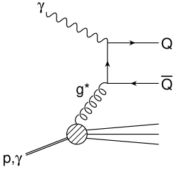
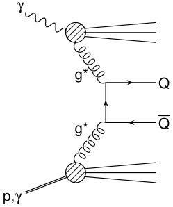
a)	b)	c)

Figure 4: Diagrams illustrating the heavy quark production in $\gamma\gamma$or $\gamma p$ collisions through different mechanisms: a) direct production (only for $\gamma\gamma$ interactions), b) photoproduction in single resolved case, where one photon or the proton is resolved, and c) double resolved case, where both incoming particles are resolved.

In the collinear limit one uses the leading twist term of the operator product expansion, neglecting the transverse momenta of the partons. The cross section for heavy quark photoproduction off one of the photons being resolved reads

$$\sigma^{cf}_{1R}(s,M^{2})=\sum_{i}\int{dx\over x}f_{i}(x,\mu^{2})\hat{\sigma}^{cf}_{\gamma i}(M^{2},xs),$$ (15)

where the partonic cross sections $\hat{\sigma}^{cf}_{\gamma i}$ are well known up to the NLO approximation and $f_{i}(x,\mu^{2})$is the parton $i$ distribution function in the photon, at the factorization scale $\mu\simeq 2M$. In the above, $s$ denotes the $\gamma\gamma$ invariant mass squared, and $M$ is the quark mass.

In the $k_{t}$ factorization formalism, the complete kinematics of the gluon-photon fusion is taken into account and the small light-cone component of the longitudinal momentum of the gluon is integrated out. Then, the cross section takes the following form

$$\sigma^{kf}_{1R}(s,M^{2})=\sum_{i}\int{dx\over x}{d^{2}\mbox{\boldmath$k$}\over\pi}{\cal F}_{i}(x,\mbox{\boldmath$k$}^{2},\mu^{2})\,\hat{\sigma}^{kf}_{\gamma i}(\mbox{\boldmath$k$}^{2},M^{2},xs),$$ (16)

in which the unintegrated parton density ${\cal F}_{i}(x,\mbox{\boldmath$k$}^{2},\mu^{2})$ and the off-shell partonic cross section $\hat{\sigma}^{kf}_{\gamma i}(\mbox{\boldmath$k$}^{2},M^{2},x_{1}x_{2}s)$ are employed. The partonic cross sections are evaluated using off-shell matrix elements. The form of $\hat{\sigma}^{kf}$ is well known in the literature, see for example [11], and we quote it in Appendix A. Formulae (15) and (16), with the appropriate substitution of parton densities, are valid also for the photoproduction off the proton. It is important to note that, in a $\gamma\gamma$ collision one or the other photon may be resolved, thus the inclusive cross section for heavy quark production acquires an additional factor of 2. At the LO approximation, only gluons contribute to the $Q\bar{Q}$ production.

The double-resolved contribution to the process $\gamma\gamma\to Q\bar{Q}X$ is described by

$$\sigma^{cf}_{2R}(s,M^{2})=\sum_{i,j}\int{dx_{1}\over x_{1}}{dx_{2}\over x_{2}}{f}_{i}(x_{1},\mu^{2}){f}_{j}(x_{2},\mu^{2})\hat{\sigma}^{cf}_{ij}(M^{2},x_{1}x_{2}s),$$ (17)

in the collinear limit and the cross section in the $k_{t}$ factorization formalism reads

$$\sigma^{kf}_{2R}(s,M^{2})=\sum_{i,j}\int{dx_{1}\over x_{1}}{dx_{2}\over x_{2}}{d^{2}\mbox{\boldmath$k$}_{1}\over\pi}{d^{2}\mbox{\boldmath$k$}_{2}\over\pi}{\cal F}_{i}(x_{1},\mbox{\boldmath$k$}_{1}^{2},\mu^{2})\,{\cal F}_{j}(x_{2},\mbox{\boldmath$k$}_{2}^{2},\mu^{2})\,\hat{\sigma}^{kf}_{ij}(\mbox{\boldmath$k$}_{1},\mbox{\boldmath$k$}_{2},M^{2},x_{1}x_{2}s),$$ (18)

where $\hat{\sigma}^{kf}_{ij}$ for gluons is given in Appendix B (following from [41]). Analogously, one of the photons may be replaced by the proton in order to obtain a resolved photon contribution to heavy quark photoproduction off the proton.

In the following, we shall restrict ourselves to the effects of transverse momentum in the gluon kinematics, and the quark contribution will only be taken in the collinear approximation. This should not affect significantly the results, as the heavy quark production is driven mostly by exchanges of gluons. For the collinear limit, all the theoretical estimates were obtained using the PYTHIA Monte Carlo [42].

4 Results for heavy quark production

The measurements of cross sections for the inclusive charm and bottom production in $e^{+}e^{-}$ and $ep$ collisions were performed at LEP and HERA respectively. For bottom production at LEP, only the total rate $e^{+}e^{-}\to e^{+}e^{-}b\bar{b}X$ was measured [8], representing an average of the $\gamma\gamma\to b\bar{b}X$cross section weighted with the flux of photons in the electrons. For charm, the cross section $\sigma(\gamma\gamma\to c\bar{c}X)$ was determined for different $\gamma\gamma$ collision energies [7]. At HERA, the cross section for $\gamma p\to b\bar{b}X$is known [5] for the collision energy averaged between $W=94$ GeV and $W=266$ GeV. The data for charm production at HERA [3] are available for virtual photons, at different virtualities $Q^{2}$ and collision energies $W$ in the form of $F_{2}^{\mathrm{c}harm}(x,Q^{2})$. We give in this section the theoretical estimates for these processes based on the $k_{t}$ factorization formalism and study the theoretical uncertainties.

4.1 Theoretical uncertainties

The cross sections for heavy quark production are described by formulae (16) and (18) with the LO partonic cross sections given by (23) and (31). The results of the numerical evaluation of these formulae depend somewhat on the model for unintegrated parton densities and the choice of parameters. We have examined the following options for different elements of the model:

The heavy quark mass $M$

is plagued by a fundamental uncertainty due to confinement of color – there are no free quarks, and consequently, there is no on-shell quark mass. The running quark mass in QCD varies with the scale. It is not clear, at which scale the quark masses in the matrix elements should be evaluated, because the virtualities of heavy quarks are different for different lines in the relevant Feynman diagrams. Thus, we shall assume for the $b$ quark that $4.5$ GeV $<M_{b}<5$ GeV and for the $c$ quark that $1.3$ GeV $<M_{c}<1.5$ GeV.

The energy scale $\bar{\mu}$

that enters the running formula of the strong coupling constant $\alpha_{s}(\bar{\mu}^{2})$ in the partonic cross section (see Appendix) is usually chosen to be of order of the typical momentum transfer characterizing the process. However, the optimal value of $\bar{\mu}$ is such, that the contribution of higher orders in the perturbative expansion is minimal. Thus, without knowledge of higher order corrections, $\bar{\mu}$ is uncertain and, in order to account for this ambiguity we considered three options: (1) $\bar{\mu}^{2}=M^{2}+\mbox{\boldmath$p$}^{2}$ (standard), (2) $\bar{\mu}^{2}=(M^{2}+\mbox{\boldmath$p$}^{2})/4$ (low scale) and (3) $\bar{\mu}^{2}=4M^{2}$ (large scale), where $\mbox{\boldmath$p$}=\mbox{\boldmath$k$}$ (gluon transverse momentum) for the gluon-photon fusion (23) and $\mbox{\boldmath$p$}=\mbox{\boldmath$k$}_{1}-\mbox{\boldmath$k$}_{2}$ for the two-gluon process (31).

Running of the coupling constant.

We use the standard one-loop running formula for $\alpha_{s}$, with four flavors. We use, as a default choice, $\Lambda_{\mathrm{Q}CD}=140$ MeV, such that $\alpha_{s}(M_{Z}^{2})=0.117$ as given by the latest QCD fits. We also test the PYTHIA default value: $\Lambda_{\mathrm{Q}CD}=250$ MeV, corresponding to the value of $\alpha_{s}(M_{Z}^{2})=0.128$.

Unintegrated parton distributions.

For the proton, we take into account the CCFM gluon distribution, as given in the CASCADE Monte Carlo [43], the unintegrated gluon obtained from the GRV and MRST parameterizations using the KMR method (uGRV and uMRST) and the gluon following from the saturation model (GBW). In the case of a real photon, the KMR method is applied to the GRS gluon (uGRS) and an alternative model of the unintegrated gluon is given by the saturation model for photons (GBW$\gamma$), as explained in Sec. 2.1. Furthermore, we vary the factorization scale in the two-scale gluon distribution ${\cal F}_{g}(x,\mbox{\boldmath$k$}^{2},\mu^{2})$ between $\mu=M$and $\mu=2M$.

Parton momentum fraction $x$.

In the collinear approximation, one neglects the non-zero transverse momentum $k$ of the incoming parton whereas in the $k_{t}$ factorization approach, the transverse momentum is included in the kinematics of partonic scattering. Thus, for the virtual photon-gluon fusion, the invariant mass of the system is $\hat{s}_{\gamma g}=xs$ in the collinear approximation and $\hat{s}^{\prime}_{\gamma g}=xs-\mbox{\boldmath$k$}^{2}$ when the complete kinematics are taken into account. In a standard approximation method, the cross section in the collinear factorization can be obtained from the one in the $k_{t}$ factorization, using a substitution $\hat{\sigma}^{kf}(xs,\mbox{\boldmath$k$}^{2},Q^{2})\rightarrow\hat{\sigma}^{kf}(xs,\mbox{\boldmath$k$}^{2}=0,Q^{2})\theta(Q^{2}-\mbox{\boldmath$k$}^{2})$, and the integrated parton distributions as defined by the eq. (1). However, such approximation neglects the fact that the kinematical threshold in DIS for $\hat{\sigma}^{kf}$ depends on $\mbox{\boldmath$k$}^{2}$, i.e. the kinematical threshold for the virtual photoproduction is located at $x\simeq Q^{2}/s$ in the collinear approximation and at

$$\bar{x}(\mbox{\boldmath$k$}^{2})\simeq(Q^{2}+\mbox{\boldmath$k$}^{2})/s\simeq x[1+\mbox{\boldmath$k$}^{2}/Q^{2}]$$ (19)

in the $k_{t}$ factorization framework.

In order to investigate the inclusion of the latter threshold treatment, the standard approximation could suffer modifications by introducing a rescaled variable $z=xQ^{2}/(Q^{2}+\mbox{\boldmath$k$}^{2})$. This will improve the approximation and lead to an alternative relation between the $k_{t}$ factorization and collinear approximation expressions, where

$$zg(z,Q^{2})=\int_{0}^{Q^{2}}d\mbox{\boldmath$k$}^{2}\;{\cal F}_{g}(z(Q^{2}+\mbox{\boldmath$k$}^{2})/Q^{2},\mbox{\boldmath$k$}^{2},Q^{2}).$$ (20)

Thus, the use of the rescaled variable is a way to quantify the ambiguity in obtaining the unintegrated gluon distribution from the integrated one.

In our investigation of the effects of the threshold treatment in the evaluation of the heavy quark production cross section, we consider a substitution

$$x^{\prime}={x\over 1+\mbox{\boldmath$k$}^{2}/(4M^{2})}$$ (21)

in the unitegrated gluon distributions ${\cal F}_{g}(x^{\prime},\mbox{\boldmath$k$}^{2},\mu^{2})$. Note, that for massive quark photoproduction, $4M^{2}$ replaces $Q^{2}$. Such rescaling is not necessary for the CCFM gluon, where the kinematical effects of the transverse momentum are already accounted for in the $F_{2}$ fits.

4.2 Results for $\gamma p$ interactions

In Fig. 5 we give a set of results for cross sections for $\gamma p\to b\bar{b}X$ with the direct photon (Fig. 5a) and with the resolved photon (Fig. 5b). The default results (full curves) are obtained by taking the CCFM unintegrated gluon in the proton (from CASCADE), $M_{b}=4.5$ GeV, $\mu=10$ GeV, $\Lambda_{\mathrm{Q}CD}=140$ MeV and the standard scale for the running coupling (see Sec. 4.1). For the gluon in the photon, the KMR method is applied to obtain the unintegrated GRS parameterization (uGRS). Besides the default choice, we also use the unintegrated GRV distribution (uGRV), based on the GRV NLO parameterization, and the GBW gluon, leaving other parameters unchanged. Furthermore, we investigate the impact of the $x$-rescaling, for the uGRV gluon (direct photon) and for both the uGRV and uGRS gluon (resolved photon). We modify the default choice of the QCD parameters: we use $\Lambda_{\mathrm{Q}CD}=250$ MeV and the low scale for running, in order to obtain an upper limit for the cross section. A very conservative estimate follows from the choice $M_{b}=5$ GeV and the large energy scale for $\alpha_{s}$. We have checked, that using the unintegrated MRST gluon and variations of the renormalization scale $\mu$ have a minor influence on the results, hence we do not include the corresponding curves in the figure.

a)
b)

Figure 5: Cross sections of $b\bar{b}$ production in $\gamma p$ interactions from the $k_{t}$ factorization approach, showing a) the single resolved contribution and b) the double resolved contribution. Details of the curves are presented in the text.

It is visible in the figure, that the contribution from the resolved photon is significant – roughly 20–30% of the direct photon cross section for the default choice of parameters. We have checked, that in all cases, the resolved photon contribution rises faster with the energy $W$ than the direct photon one. The results are rather stable against modifications of the unintegrated gluon and the quark mass. The largest contribution to the uncertainty of the cross section comes from the details of the QCD running of $\alpha_{s}$ and the choice of energy scale – reflecting a potential influence of higher order corrections. When the low scale of $\alpha_{s}$and the large value of $\Lambda_{\mathrm{Q}CD}$ are assumed, the direct contribution gets enhanced by about 50% and the resolved one gets doubled. In this extreme case, the calculation results for the sum of the direct and resolved photon cross sections $\sigma(W=180$ GeV)$=143$ nb is close to the experimental data point $\sigma=206\pm 19^{+46}_{-40}$ nb (see Fig. 6). Thus, although the QCD predictions are significantly lower than the data, inconsistency cannot be claimed, due to the large experimental error and the large theoretical uncertainty coming from uncontrolled higher order corrections.

a)	b)

Figure 6: Comparison between the collinear factorization and the $k_{t}$factorization approaches to $b\bar{b}$ production in $\gamma p$ interactions. Shown are the experimental data from EMC [4] and H1 [5]. a) The total $b\bar{b}$ cross section in the $k_{t}$ factorization (solid line) includes single and double resolved contributions. In the collinear factorization, the total cross section (short dashed) also includes the specific contribution from the $q\bar{q}$ annihilation for the double resolved case (long dashed). b) Comparison between the single resolved components in the $k_{t}$ (solid line) and collinear (short dashed) factorizations, and between the double resolved components in the $k_{t}$ (dotted) and collinear (long dashed) factorizations.

The saturation model estimate of the direct photon contribution to bottom production is lower than the default result. The double resolved contribution obtained using the GBW parameterization for both the photon and the proton is slightly larger than its KMR counterpart. The constraint we have imposed on the parton density at large $x$ via the threshold factor plays a very important role for the resolved photon case, being dependent on the gluon at relatively large $x$. The consistency of the standard QCD and saturation model results is not surprising, as both sets of parameterizations are constrained by the same experimental data (see Fig. 2). It is, however, striking that the unintegrated GBW gluon leads to a lower cross section than the uGRS gluon, while giving higher integrated distribution, as shown in Fig. 2. This effect is caused by strong suppression of the GBW gluon at transverse momenta larger than the saturation scale, as we demonstrated in Fig. 3b.

In Fig. 6a we show results for the total cross section, $\sigma(\gamma p\to b\bar{b}X)$ obtained in the $k_{t}$ factorization formalism and in the collinear approximation, compared to the experimental data. In both cases, the direct and resolved photon contributions are added. The resolved photon contribution, coming from the partonic process $q\bar{q}\to Q\bar{Q}$is only evaluated in the collinear limit and demonstrated to be negligibly small. In Fig. 6b, the cross sections are decomposed into the direct and resolved photon components.

Figure 7: The structure function $F_{2}^{c\bar{c}}$ as a function of $x$ at different values of $Q^{2}$ between 1.8 GeV² and 130 GeV². The continuous lines represent the results from the saturation model, with the parameters from [32], compared with the experimental results from ZEUS [3].

We used the unintegrated gluon in the proton obtained via the KMR method (uGRV) and the default values of the other parameters for the $k_{t}$ factorization calculation, as given in Sec. 4.2. The collinear limit results are obtained using the corresponding integrated gluon distributions (GRV), transverse momenta are set to zero in the definition of energy scale for $\alpha_{s}$, that is we take $\alpha_{s}(M^{2})$. Other parameters take their default values. Therefore, we gain insight into the actual difference between the studied approximations, not caused by discrepancy of input parameters. Thus, it is clear from Fig. 6b, that a large enhancement (by a factor of three) of the resolved photon cross section occurs due to non-zero transverse momentum effects, whereas the direct photon contribution gains only modest 10–20% in the magnitude. The total cross section is larger by some 20–30% in the $k_{t}$ factorization approach.

It has been checked that charm production at HERA is well described within the $k_{t}$ factorization approach[44]. For completeness, we show in Fig. 7 our results for the charm structure function $F_{2}^{\mathrm{c}harm}(x,Q^{2})$, based on the standard saturation model, compared to experimental data. The quark mass $M_{c}=1.3$ GeV. The agreement of the theory and the data is very good, in contrast to the discussed bottom production case. The results we have obtained for bottom production in the single resolved case are compatible with previous studies of heavy quark production using the $k_{t}$ factorization approach [14, 18]. These studies found agreement with the first erroneous data point from HERA [5], which gave a cross section for bottom production lower by a factor 2 than found later [5]. With the inclusion of the resolved photon in the $k_{t}$ factorization framework, we restore a similar level of agreement with the experimental data.

4.3 Results for $\gamma\gamma$ interactions

a)
b)

Figure 8: Cross sections of $b\bar{b}$ production in $\gamma\gamma$ interactions from the $k_{t}$ factorization approach, showing a) the single resolved contribution and b) the double resolved contribution. Details of the curves are presented in the text.

The default set of parameters for bottom production in $\gamma\gamma$ collisions is the same as it was in the case of the $\gamma p$ process. The unintegrated gluon in the photon is unfolded from the GRS parameterization, using the KMR method (see Sec. 2.1). We investigate the sensitivity of the cross section to variations of the parameters. The results are shown as a function of $\gamma\gamma$ energy $W$ in Fig. 8. The default results (continuous line) are compared with the results incorporating the kinematical rescaling of $x$ (see Sec. 4.1). Besides that, the low scale in the running formula of $\alpha_{s}$ and the large $\Lambda_{\mathrm{Q}CD}$are assumed and the case of $M_{b}=5.0$ GeV and the large scale of $\alpha_{s}$ is shown. Furthermore, the unintegrated gluon in the photon from the saturation model is used. We stress that within the presented $W$ range, the results are driven by the gluon at relatively large $x\sim 0.1$, where the saturation model is less reliable and phenomenological threshold factors need to be imposed.

a)	b)

Figure 9: Comparison between the collinear factorization and the $k_{t}$ factorization approaches to $b\bar{b}$ production in $\gamma\gamma$interactions. a) The total $b\bar{b}$ cross section is represented with the solid line in the $k_{t}$ factorization and with the short dashed line in the collinear factorization. The long dashed line gives the specific contribution from the $q\bar{q}$ annihilation in the double resolved case, corresponding to the collinear approach. The dotted line shows the contribution from the quark box (see Fig. 4a). b) Comparison between the single resolved components in the $k_{t}$ (solid line) and collinear (short dashed) factorizations, and between the double resolved components in the $k_{t}$ (dotted) and collinear (long dashed) factorizations.

Furthermore in Fig. 9, we illustrate the enhancement of the cross sections due to non-zero transverse momentum of the gluon. This figure is constructed in strict analogy to Fig. 6 discussed in Sec. 4.2. The conclusions from these results are also very similar to those obtained in the $\gamma p$ case. Let us only mention, that the integrated and unintegrated GRS parameterization of the gluon in the photon was used. Note, that the QPM contribution (see the diagram in Fig. 4a) shown in Fig. 9a is included in the total cross sections $\sigma(\gamma\gamma\to b\bar{b}X)$. In order to obtain the total cross section $\sigma(e^{+}e^{-}\to e^{+}e^{-}b\bar{b}X)$, the $\gamma\gamma$ cross section needs to be weighted with the photon flux in the electrons. Thus, we obtained the value of $\sigma(e^{+}e^{-}\to e^{+}e^{-}b\bar{b}X)=1.9$ pb for the default case (based on KMR gluon density), while the use of the GBW gluons gives $\sigma(e^{+}e^{-}\to e^{+}e^{-}b\bar{b}X)=2.7$ pb. The latter value is lower than what we previously found using a generalization of the saturation model [32], with the difference coming from the threshold factor imposed at the level of the unintegrated gluon ${\cal F}_{g}(x,\mbox{\boldmath$k$}^{2})$instead of the total cross section. The behavior of the cross section in the vicinity of the kinematic threshold is crucial for interpretation of the LEP measurements of bottom production. An interesting discussion of this problem may be found in [17].

The general picture, which emerges, may be summarized with the following. The theoretical uncertainty of the QCD results for bottom production is rather large — of the order of $50\%$ for the single resolved case and, even larger for both photons resolved. The double resolved photon contribution is only a small correction (a few percent) to the single resolved photon over the studied energy range. The QCD models give results 2 times smaller than the GBW-model. The total cross section following from the $k_{t}$ factorization scheme are not significantly larger than the ones obtained in the collinear limit. Therefore, the enhancement due to the use of unintegrated gluon is not sufficient to solve the $b$-excess puzzle in $\gamma\gamma$ collisions.

a)
b)

Figure 10: Cross sections of $c\bar{c}$ production in $\gamma\gamma$ interactions from the $k_{t}$ factorization approach, showing a) the single resolved contribution and b) the double resolved contribution. Details of the curves are presented in the text.

In an analogous scheme as for the bottom, we present in Fig. 10 the results for $\sigma(\gamma\gamma\to c\bar{c}X)$. Because of the lower quark mass, the uncertainties related to the energy scale choice and the definition of gluonic $x$ are larger than for the bottom production. The double resolved photon contribution is again small, few percent correction to the dominant single resolved photon contribution. The data points are fitted well within the uncertainty band of theoretical estimates, as seen in Fig. 11. The extended GBW model as introduced in [32] and QCD give similar results for charm within the shown energy range, whereas in the bottom case the GBW gluon gave a larger cross section than QCD. The main reason of this difference is that, within the considered range of energies, the gluon is probed at lower $x$ for charm, as compared to the bottom case.

Figure 11: Cross section for the inclusive charm production in $\gamma\gamma$collisions. The data from the L3 experiment [7] are compared with the outcome of the $k_{t}$ factorization. The solid line represents our default choice for scales and parameterizations of the gluon in the photon, summing all contributions. The dashed line and the dotted line give the uncertainty due to the choice of scale. The dashed-dotted line represents our previous calculation [32] using the generalized saturation model.

5 Discussion

The main goal of this study is to investigate whether the puzzle of bottom production excess in $\gamma p$ and $\gamma\gamma$ collisions may be naturally explained in the $k_{t}$ factorization framework. Thus, we have estimated the cross sections for direct and resolved photon(s) and compared the results to their counterparts in standard collinear approximations.

We, indeed, found some enhancement of the cross section for a direct photon scattering off both the proton and the resolved photon. This effect itself is too small, though, to get the theory results close to the experimental data. Furthermore, we showed, that the cross sections driven by two-gluon fusion are substantially larger (by a factor of 2–3) when the unintegrated gluon is used. Despite this enhancement, these subprocesses contribute only as a 20–30% correction to the total cross section for bottom production in the $\gamma p$ collisions, and less than 10% for $\gamma\gamma$.

The sensitivity of the results to various model uncertainties is found to be large. Thus, in the marginal case, the theoretical results for $\gamma p\to b\bar{b}X$ in the $k_{t}$ factorization framework, is enhanced and agrees with the H1 data point within errors. We do not interpret this as a strong indication of consistency between data and the theory, but rather as a consequence of the wide uncertainty band. Better understanding of higher order corrections is crucial to determine whether the H1 data point contradicts QCD results.

The picture is much more clear for $\gamma\gamma\to b\bar{b}X$. This process is dominated by the QED box diagram at low energies and by the single resolved photon mechanism at larger energies. Irrespectively of the assumption made within our framework, the emerging results for $e^{+}e^{-}\to e^{+}e^{-}b\bar{b}X$, $\sigma^{th}=1.9$ pb at the $e^{+}e^{-}$ collision energy $\sqrt{s}=200$ GeV, are more than three standard deviations below the experimental data, $13.1\pm 2.0\,{\rm(stat)}\pm 2.4\,{\rm(syst)}$ pb [8]. Thus, in the standard QCD+QED approach, the $b$ production in $e^{+}e^{-}$ collisions is hard to explain.

Interestingly enough, the agreement between the theory and the experimental data is good for the charm case both for $\gamma\gamma$ and $\gamma^{*}p$. The very different behavior of charm and bottom cross sections is surprising and calls for an explanation.

6 Conclusions

In this study we have analyzed photoproduction of heavy flavors in $\gamma\gamma$ and $\gamma p$ collisions using the $k_{t}$ factorization approach. First, we obtained parameterizations of unintegrated gluon in the photon using the KMR method. We compared features of the unintegrated gluon in the photon and in the proton. Furthermore, we proposed a parameterization of the gluon in the photon based on a generalization of the saturation model.

The parameterizations, combined with off-shell matrix elements, were used to estimate cross sections for charm and bottom production, including contributions from resolved photon. The impact of non-zero transverse momentum of gluons was studied. Some enhancement of the cross section was found in the $k_{t}$ factorization approach. In particular, we demonstrated the importance of the resolved photon contribution to bottom production in $\gamma p$ collisions. Sensitivity of the theoretical estimates to the details of the model was investigated. The conclusion is, that the use of $k_{t}$ factorization approach brings the theoretical results for bottom production closer to the data, but large discrepancies remain. For $\gamma p$ collisions, a major inconsistency cannot be claimed, because of large experimental errors and theoretical uncertainties. For the $\gamma\gamma$ case, the $b$-production excess is statistically significant, despite the uncertainties. The $k_{t}$ approach, based on QCD, does not agree with the data from LEP at the three sigma level. On the contrary, the charm production is well understood within QCD.

Thus, an interesting question arises, why the $b$-quark production excess is found in various processes. A potential explanation may be, perhaps, provided by higher order corrections. Still, it is not clear why similar, or even more important, corrections would not affect charm production in a similar way. It is also interesting to ask about uncertainties of parton densities in the photon since the experimental constraints from measurements of the photon structure and a jet photoproduction are not very stringent. Definitely, an attempt should be made to perform a new global fit of parton densities in the photon, including the bottom production data. Another interesting explanation of the $b$-excess at the Tevatron was suggested in [45] where the non-perturbative fragmentation function of the $b$ quark into $B$ mesons was updated by fitting to precise LEP data. It was found, that the discrepancy between standard theoretical calculations and the Tevatron data is significantly reduced when the improved model of fragmentation is used. Finally, there is also a possibility, that the answer to the question leads beyond QCD[46]. Therefore, it is important to further constrain theoretical uncertainties of bottom production rate estimates in QCD.

Appendix A Virtual gluon-photon fusion

The partonic cross section for an off-shell gluon with the transverse momentum $k$depend on the density matrix for gluon polarizations $\varepsilon^{\mu}(\mbox{\boldmath$k$})$. In this study, we assume that the gluons have the BFKL-like polarization tensor, that is

$$\sum_{\lambda}\epsilon^{\mu}_{\lambda}{\epsilon^{\nu}_{\lambda}}^{*}={\mbox{\boldmath$k$}^{\mu}\mbox{\boldmath$k$}^{\nu}\over\mbox{\boldmath$k$}^{2}}.$$ (22)

The result of the integration over the phase for an off-shell matrix element describing a gluon-photon fusion $\gamma(p)g^{*}(k)\to Q\bar{Q}$ is well known. We quote the result from [11]

$$\hat{\sigma}^{kf}_{\gamma g}(\mbox{\boldmath$k$}^{2},M^{2},\nu)={\pi\alpha_{em}e_{Q}^{2}\alpha_{s}(\bar{\mu}^{2})\over 2M^{2}}\Theta(\nu-4M^{2}-\mbox{\boldmath$k$}^{2})\rho\beta\left\{[(1+\rho-\frac{1}{2}\rho^{2})\,L(\beta)-1-\rho]\right.$$

$$\left.+[8+\rho-(2+3\rho)L(\beta)]\frac{\mbox{\boldmath$k$}^{2}}{\nu}+[-8+2L(\beta)]\left(\frac{\mbox{\boldmath$k$}^{2}}{\nu}\right)^{2}\right\}$$ (23)

with

$$\nu=2\,p\cdot k,\qquad\rho={4M^{2}\over\nu},$$ (24)

$$\beta=\sqrt{1-\rho\left(1-{\mbox{\boldmath$k$}^{2}\over\nu}\right)^{-1}}$$ (25)

and

$$L(\beta)={1\over\beta}\log{1+\beta\over 1-\beta}.$$ (26)

The heavy quark charge is denoted by $e_{Q}$.

Appendix B Cross sections for virtual gluons

In this appendix, we follow conventions of [41], with some minor modifications. The kinematics of the gluon fusion process $g^{*}(k_{1})+g^{*}(k_{2})\longrightarrow Q(p_{4})+\bar{Q}(p_{3})$, with respect to the four-vectors $p_{1}$ and $p_{2}$ of the incoming photons/hadrons, are given by

$$k_{1} = x_{1}p_{1}+\mbox{\boldmath$k$}_{1},$$

$$k_{2} = x_{2}p_{2}-\mbox{\boldmath$k$}_{2},$$

$$p_{3} = (1-z_{1})x_{1}p_{1}+z_{2}x_{2}p_{2}+\mbox{\boldmath$k$}_{1}-\mbox{\boldmath$\Delta$},$$

$$p_{4} = z_{1}x_{1}p_{1}+(1-z_{2})x_{2}p_{2}-\mbox{\boldmath$k$}_{2}+\mbox{\boldmath$\Delta$}.$$ (27)

The two-body phase space $d\Phi^{(2)}$ of the $Q\bar{Q}$ pair can be written in the following way

$$d\Phi^{(2)}=\frac{1}{8\pi^{2}}\frac{dz_{1}}{z_{1}(1-z_{1})}\,d^{2}\tilde{\mbox{\boldmath$\Delta$}}\,\delta\left(\nu-\frac{\tilde{\mbox{\boldmath$\Delta$}}^{2}+M^{2}}{z_{1}(1-z_{1})}-\mbox{\boldmath$q$}^{2}\right),$$ (28)

where

$$q = \mbox{\boldmath$k$}_{1}-\mbox{\boldmath$k$}_{2},$$

$$\nu = x_{1}x_{2}(2p_{1}\cdot p_{2})=\hat{s}+\mbox{\boldmath$q$}^{2},$$

$$\tilde{\mbox{\boldmath$\Delta$}} = \mbox{\boldmath$\Delta$}-\mbox{\boldmath$k$}_{1}z_{1}-\mbox{\boldmath$k$}_{2}(1-z_{1}).$$ (29)

Furthermore, the following relations hold

$$\hat{s} = \frac{\tilde{\mbox{\boldmath$\Delta$}}^{2}+M^{2}}{z_{1}(1-z_{1})},$$

$$M^{2}-\hat{t} = z_{1}(\hat{s}+{\mbox{\boldmath$k$}_{1}}^{2})+(1-z_{1}){\mbox{\boldmath$k$}_{2}}^{2}+2\tilde{\mbox{\boldmath$\Delta$}}\cdot{\mbox{\boldmath$k$}_{2}},$$

$$M^{2}-\hat{u} = (1-z_{1})(\hat{s}+{\mbox{\boldmath$k$}_{1}}^{2})+z_{1}{\mbox{\boldmath$k$}_{2}}^{2}-2\tilde{\mbox{\boldmath$\Delta$}}\cdot{\mbox{\boldmath$k$}_{2}},$$

$$z_{2} = \frac{[(1-z_{1})\mbox{\boldmath$q$}-\tilde{\mbox{\boldmath$\Delta$}}]^{2}+M^{2}}{(1-z_{1})\nu},$$

$$1-z_{2} = \frac{[z_{1}\mbox{\boldmath$q$}+\tilde{\mbox{\boldmath$\Delta$}}]^{2}+M^{2}}{z_{1}\nu}.$$ (30)

In this notation, the cross section $\hat{\sigma}^{kf}_{gg}(\mbox{\boldmath$k$}_{1},\mbox{\boldmath$k$}_{2},M^{2},\nu)$for production of heavy quarks in two-gluon collisions $g^{*}g^{*}\to Q\bar{Q}$ equals (from [41])

$$\hat{\sigma}^{kf}_{gg}(\mbox{\boldmath$k$}_{1},\mbox{\boldmath$k$}_{2},M^{2},\nu)=\frac{4\pi^{2}}{N_{c}^{2}-1}\nu\alpha_{s}^{2}(\bar{\mu}^{2})\int d\Phi^{(2)}D(\mbox{\boldmath$k$}_{1},\mbox{\boldmath$k$}_{2},\nu,\mbox{\boldmath$\Delta$},z_{1},M^{2}),$$ (31)

and the matrix element $D(\mbox{\boldmath$k$}_{1},\mbox{\boldmath$k$}_{2},\nu,\mbox{\boldmath$\Delta$},z_{1},M^{2})$ is given by

$$D = \frac{1}{N_{c}}\left[\frac{-1}{(M^{2}-\hat{u})(M^{2}-\hat{t})}+\frac{(B+C)^{2}}{{\mbox{\boldmath$k$}_{1}}^{2}{\mbox{\boldmath$k$}_{2}}^{2}}\right]+$$ (32)

$$+ N_{c}\left[\frac{1}{\hat{s}}\left(\frac{1}{M^{2}-\hat{t}}-\frac{1}{M^{2}-\hat{u}}\right)(1-z_{1}-z_{2})-\frac{B^{2}+C^{2}}{{\mbox{\boldmath$k$}_{1}}^{2}{\mbox{\boldmath$k$}_{2}}^{2}}\right.+$$

$$\hphantom{N_{c}\Bigg{[}}\!\left.+\frac{2(B-C)}{{\mbox{\boldmath$k$}_{1}}^{2}{\mbox{\boldmath$k$}_{2}}^{2}\hat{s}}\left((1-z_{2}){\mbox{\boldmath$k$}_{1}}^{2}+(1-z_{1}){\mbox{\boldmath$k$}_{2}}^{2}+{\mbox{\boldmath$k$}_{1}}\cdot{\mbox{\boldmath$k$}_{2}}\right)\right]+$$

$$+ N_{c}\left[\frac{2}{\nu\hat{s}}-\frac{2}{{\mbox{\boldmath$k$}_{1}}^{2}{\mbox{\boldmath$k$}_{2}}^{2}}\frac{\left((1-z_{2}){\mbox{\boldmath$k$}_{1}}^{2}+(1-z_{1}){\mbox{\boldmath$k$}_{2}}^{2}+{\mbox{\boldmath$k$}_{1}}\cdot{\mbox{\boldmath$k$}_{2}}\right)^{2}}{\hat{s}^{2}}\right],$$

where the following notation has been used

$$B = \frac{1}{2}-\frac{(1-z_{1})(1-z_{2})\nu}{M^{2}-\hat{u}}+\frac{\nu(1-z_{1}-z_{2})}{2\hat{s}}+\frac{\mbox{\boldmath$\Delta$}\cdot({\mbox{\boldmath$k$}_{1}}+{\mbox{\boldmath$k$}_{2}})}{\hat{s}},$$

$$C = \frac{1}{2}-\frac{z_{1}z_{2}\nu}{M^{2}-\hat{t}}-\frac{\nu(1-z_{1}-z_{2})}{2\hat{s}}-\frac{\mbox{\boldmath$\Delta$}\cdot({\mbox{\boldmath$k$}_{1}}+{\mbox{\boldmath$k$}_{2}})}{\hat{s}}.$$ (33)

References

- [1] F. Abe et al. [CDF Collaboration], Phys. Rev. Lett. 71 (1993) 500; 71 (1993) 2396; 75 (1995) 1451; B. Abbott et al. [D0 Collaboration], Phys. Lett. B 487 (2000) 264.
- [2] J. Breitweg et al. [ZEUS Collaboration], Eur. Phys. J. C 6 (1999) 67; C. Adloff et al. [H1 Collaboration], Nucl. Phys. B 545 (1999) 21.
- [3] J. Breitweg et al. [ZEUS Collaboration], Eur. Phys. J. C 12 (2000) 35.
- [4] J. J. Aubert et al. [European Muon Collaboration], Phys. Lett. B 106 (1981) 419.
- [5] C. Adloff et al. [H1 Collaboration], Phys. Lett. B 467 (1999) 156; Erratum-ibid. B 518 (2001) 331.
- [6] J. Breitweg et al. [ZEUS Collaboration], Eur. Phys. J. C 18 (2001) 625.
- [7] M. Acciarri et al. [L3 Collaboration], Phys. Lett. B 514 (2001) 19.
- [8] M. Acciarri et al. [L3 Collaboration], Phys. Lett. B 503 (2001) 10; The OPAL Collaboration, OPAL Physics Note PN455.
- [9] S. Frixione and P. Nason, JHEP 0203 (2002) 053.
- [10] J. C. Collins and R. K. Ellis, Nucl. Phys. B 360 (1991) 3.
- [11] S. Catani, M. Ciafaloni and F. Hautmann, Nucl. Phys. B 366 (1991) 135.
- [12] E. M. Levin, M. G. Ryskin, Y. M. Shabelski and A. G. Shuvaev, Sov. J. Nucl. Phys. 53 (1991) 657; 54 (1991) 867.
- [13] M. G. Ryskin, A. G. Shuvaev and Y. M. Shabelski, Phys. Atom. Nucl. 64 (2001) 1995.
- [14] A. V. Lipatov, V. A. Saleev and N. P. Zotov, Mod. Phys. Lett. A 15 (2000) 1727.
- [15] A. V. Lipatov, V. A. Saleev and N. P. Zotov, hep-ph/0112114.
- [16] H. Jung, Phys. Rev. D 65 (2002) 034015.
- [17] A. Szczurek, hep-ph/0203050.
- [18] C. B. Mariotto, M. B. Ducati and M. V. Machado, hep-ph/0208155.
- [19] G. Marchesini and B. R. Webber, Nucl. Phys. B 386 (1992) 215; S. Catani and F. Hautmann, Nucl. Phys. B 427 (1994) 475.
- [20] B. Andersson et al. [Small x Collaboration], Eur. Phys. J. C 25 (2002) 77.
- [21] L. N. Lipatov, Sov. J. Nucl. Phys. 23 (1976) 338; E. A. Kuraev, L. N. Lipatov and V. S. Fadin, Sov. Phys. JETP 44, 443 (1976); ibid. 45 (1977) 199; I. I. Balitsky and L. N. Lipatov, Sov. J. Nucl. Phys. 28 (1978) 822.
- [22] M. Ciafaloni, Nucl. Phys. B 296 (1988) 49; S. Catani, F. Fiorani and G. Marchesini, Phys. Lett. B 234 (1990) 339; Nucl. Phys. B 336 (1990) 18; G. Marchesini, Nucl. Phys. B 445 (1995) 49.
- [23] J. Kwieciński, A. D. Martin and A. M. Staśto, Phys. Rev. D 56 (1997) 3991.
- [24] H. Jung and G. P. Salam, Eur. Phys. J. C 19 (2001) 351.
- [25] M. A. Kimber, J. Kwieciński, A. D. Martin and A. M. Staśto, Phys. Rev. D 62 (2000) 094006.
- [26] M. A. Kimber, A. D. Martin and M. G. Ryskin, Phys. Rev. D 63 (2001) 114027.
- [27] M. A. Kimber, A. D. Martin and M. G. Ryskin, Eur. Phys. J. C 12 (2000) 655.
- [28] K. Golec-Biernat and M. Wüsthoff, Phys. Rev. D 59 (1999) 014017; 60 (1999) 114023.
- [29] N. Tîmneanu, presentation at the Small-x workshop, Lund, June 2002
- [30] A. I. Shoshi, F. D. Steffen, H. G. Dosch and H. J. Pirner, hep-ph/0207287.
- [31] A. Gawron and J. Kwieciński, hep-ph/0207299.
- [32] N. Tîmneanu, J. Kwieciński and L. Motyka, Eur. Phys. J. C 23 (2002) 513.
- [33] V. Gribov and L. Lipatov, Sov. J. Nucl. Phys. 15 (1972) 438 and 675; L. Lipatov Sov. J. Nucl. Phys. 20 (1975) 94; G. Altarelli and G. Parisi, Nucl. Phys. B 126 (1977) 298; Y. Dokshitser, Sov. Phys. JETP 46 (1977)641.
- [34] Y. L. Dokshitzer, D. Diakonov and S. I. Troian, Phys. Rept. 58 (1980) 269.
- [35] M. Glück, E. Reya and I. Schienbein, Phys. Rev. D 60 (1999) 054019.
- [36] M. Glück, E. Reya and I. Schienbein, Eur. Phys. J. C 10 (1999) 313.
- [37] J. Kwieciński, hep-ph/0203172.
- [38] M. Glück, E. Reya and A. Vogt, Eur. Phys. J. C 5 (1998) 461.
- [39] C. Adloff et al. [H1 Collaboration], Phys. Lett. B 483 (2000) 36.
- [40] V. M. Budnev, I. F. Ginzburg, G. V. Meledin and V. G. Serbo, Phys. Rept. 15 (1974) 181.
- [41] R. D. Ball and R. K. Ellis, JHEP 0105 (2001) 053.
- [42] T. Sjöstrand et al., Comput. Phys. Commun. 135 (2001) 238.
- [43] H. Jung, Comput. Phys. Commun. 143 (2002) 100.
- [44] S. P. Baranov, H. Jung, L. Jonsson, S. Padhi, N. P. Zotov, Eur. Phys. J. C 24 (2002) 425.
- [45] M. Cacciari and P. Nason, Phys. Rev. Lett. 89 (2002) 122003.
- [46] E. L. Berger, B. W. Harris, D. E. Kaplan, Z. Sullivan, T. M. Tait and C. E. Wagner, Phys. Rev. Lett. 86 (2001) 4231.