Light-flavor sea-quark distributions in the nucleon
in the SU(3) chiral quark soliton model (I)
— phenomenological predictions —

Abstract

Theoretical predictions are given for the light-flavor sea-quark distributions in the nucleon including the strange quark ones on the basis of the flavor SU(3) version of the chiral quark soliton model. Careful account is taken of the SU(3) symmetry breaking effects due to the mass difference $\Delta m_{s}$ between the strange and nonstrange quarks, which is the only one parameter necessary for the flavor SU(3) generalization of the model. A particular emphasis of study is put on the light-flavor sea-quark asymmetry as exemplified by the observables $\bar{d}(x)-\bar{u}(x),\bar{d}(x)/\bar{u}(x),\Delta\bar{u}(x)-\Delta\bar{d}(x)$ as well as on the particle-antiparticle asymmetry of the strange quark distributions represented by $s(x)-\bar{s}(x),s(x)/\bar{s}(x),\Delta s(x)-\Delta\bar{s}(x)$ etc. As for the unpolarized sea-quark distributions, the predictions of the model seem qualitatively consistent with the available phenomenological information provided by the NMC data for $\bar{d}(x)-\bar{u}(x)$, the E866 data for $\bar{d}(x)/\bar{u}(x)$, the CCFR data and Barone et al.’s fit for $s(x)/\bar{s}(x)$ etc. The model is shown to give several unique predictions also for the spin-dependent sea-quark distribution, such that $\Delta s(x)\ll\Delta\bar{s}(x)\lesssim 0$ and $\Delta\bar{d}(x)<0<\Delta\bar{u}(x)$, although the verification of these predictions must await more elaborate experimental investigations in the near future.

I Introduction

As is widely known, the perturbative QCD can predict only the $Q^{2}$-dependence of parton distribution functions (PDF), whereas it can say nothing about the PDF at a prescribed energy scale. To predict PDF themselves, we need to solve nonperturbative QCD, which is an extremely difficult theoretical problem. It cannot be denied that, at least at the present stage, we cannot be too much ambitious in this respect. Still, we can do qualitatively interesting investigations. The key observation here is the following. In their semi-phenomenological analyses of PDF, Glück, Reya and Vogt prepared the initial PDF at fairly low energy scale around 600 MeV, in contrast to the standard consent of perturbative QCD, and they concluded that light-flavor sea-quark (or antiquark) components are absolutely necessary even at this relatively low energy scale GRV95 ,GRSV96 . Furthermore, even the flavor asymmetry of the sea-quark distributions have been established by the celebrated NMC measurement NMC91 . The origin of this sea-quark asymmetry seems definitely nonperturbative, and cannot be explained by the sea-quarks radiatively generated through the perturbative QCD evolution processes. Here we certainly need some low energy (nonperturbative) mechanism which generates sea-quark distributions in the nucleon. In our opinion, the chiral quark soliton model (CQSM) is the simplest and most powerful effective model of QCD, which fulfills the above physical requirement DPP88 –DP01 . Although it may still be a toy model in the sense that the gluon degrees of freedom are only implicitly handled, it has several nice features that are not shared by other effective models like the MIT bag model. Among others, most important in the above-explained context is its field theoretical nature, i.e. the proper account of the polarization of Dirac sea quarks, which enables us to make reasonable estimation not only of quark distributions but also of antiquark distributions DPPPW96 –WK99 . It has already been shown that, without introducing any adjustable parameter, except for the initial-energy scale of the $Q^{2}$-evolution, the CQSM can describe nearly all the qualitatively noticeable features of the recent high-energy deep-inelastic scattering observables. It naturally explains the NMC observation, i.e. the excess of $\bar{d}$-sea over the $\bar{u}$-sea in the proton WK98 ,W91A –W92 , PPGWW99 . It also reproduces the characteristic features of the observed longitudinally polarized structure functions of the proton, the neutron and the deuteron WK99 ,WW00A . Even the most puzzling observation, i.e. the unexpectedly small quark spin fraction of the nucleon, can be explained at least qualitatively with no need of a large gluon polarization at the low renormalization scale WY91 ,WW00B . Finally, the model predicts a sizably large isospin asymmetry also for the spin-dependent sea-quark distributions, which we expect will be confirmed by near future experiments DPPPW96 ,WK99 ,WW00A ,DGPW00 .

The above-mentioned unique feature of the CQSM is believed to play important roles also in the study of hidden strange quark excitations in the nucleon, which entirely have non-valence character W02 . The main purpose of the present study is to give theoretical predictions for both of the unpolarized and the longitudinally polarized strange quark distributions in the nucleon, on the basis of the CQSM generalized to the case of flavor SU(3). Naturally, because of fairly large mass difference between the strange and nonstrange quarks, the flavor SU(3) symmetry is not so perfect symmetry as the flavor SU(2) one is. We must take account of this symmetry breaking effects in some way or other. Here, we shall accomplish it relying upon the first order perturbation theory. It should be emphasized that, in our effective theory at quark level, this effective mass difference $\Delta m_{s}$ between the $s$-quark and the $u,d$-quarks is the only one additional parameter necessary for the flavor SU(3) generalization of the CQSM. Through the study outlined above, we will be able to answer several interesting questions as follows. How important in nature is the admixture or the virtual excitation of $s$-$\bar{s}$ pairs in the nucleon, a system of total strange-quantum-number being zero? Does the asymmetry of the $s$-quark and $\bar{s}$-quark distributions exist at all? If it exists, how large is it? Do we expect an appreciable particle-antiparticle asymmetry also for the spin-dependent strange quark distribution? We also want to verify whether a favorable prediction of the flavor SU(2) CQSM, i.e. the excess of the $\bar{d}$-sea over the $\bar{u}$-sea in the proton, is taken over by the SU(3) model or not. What answer do we obtain for the isospin asymmetry of the spin dependent sea-quark distributions $\Delta\bar{u}(x)-\Delta\bar{d}(x)$ in the flavor SU(3) CQSM?

In consideration of the length of the theoretical formulation of the model, we think it more appropriate to organize the paper as follows. That is, for the benefit of readers who have interest only in the phenomenological consequences of the SU(3) CQSM, we leave the description of the full theoretical formalism to a separate paper. (This paper will hereafter be referred to as II.) Instead, we will give in next section a brief summary of what dynamical assumptions the model is constructed on and what approximations are necessary there. Next, in sect.3, we compare the theoretical predictions of the model with available phenomenological information. We shall also give some discussions on the physical origin of the unique predictions of the model as to the light-flavor sea-quark asymmetry. Finally, in sect.4, some concluding remarks will made.

II A brief summary of the model

Since the flavor $SU(3)$ CQSM is constructed on the basis of the flavor $SU(2)$ model, we first recall some basics of the $SU(2)$ CQSM. It is specified by the effective Lagrangian DPP88 ,

$${\cal L}\ =\ \bar{\psi}(x)(\,i\!\not\!\partial-MU^{\gamma_{5}}(x)\,)\psi(x).$$ (1)

with

$$U^{\gamma_{5}}(x)\ =\ e^{i\gamma_{5}\pi(x)/f_{\pi}},\hskip 42.67912pt\pi(x)=\pi_{a}(x)\tau_{a}\ \ \ (a=1,\cdots,3)$$ (2)

which describes the effective quark fields with a dynamically generated mass $M$, interacting with massless pions. The nucleon (or $\Delta$) in this model appears as a rotational state of a symmetry-breaking hedgehog object, which itself is obtained as a solution of the self-consistent Hartree problem with infinitely many Dirac-sea quarks DPP88 ,WY91 . The theory is not renormalizable, and it is defined with an ultraviolet cutoff. In the Pauli-Villars regularization scheme, which is used throughout the present analysis, that which plays the role of the ultraviolet cutoff is the Pauli-Villars mass $M_{PV}$ obeying the relation $\left(N_{c}M^{2}/4\pi^{2}\right)\ln{\left(M_{PV}/M\right)}^{2}=f_{\pi}^{2}$ with $f_{\pi}$ the pion weak decay constant DPPPW96 . Using the value $M\simeq 375\,\mbox{MeV}$, which is obtained from the phenomenology of nucleon low energy observables, this relation fixes the Pauli-Villars mass as $M_{PV}\simeq 562\,\mbox{MeV}$. Since we are to use these values of $M$ and $M_{PV}$, there is no free parameter additionally introduced into the calculation of distribution functions WW00A .

The basic lagrangian of the SU(3) CQSM is given as

$${\cal L}\ =\ \bar{\psi}(x)(\,i\!\not\!\partial-MU^{\gamma_{5}}(x)-\Delta m_{s}P_{s}\,)\psi(x).$$ (3)

with

$$U^{\gamma_{5}}(x)\ =\ e^{i\gamma_{5}\pi(x)/f_{\pi}},\hskip 42.67912pt\pi(x)=\pi_{a}(x)\lambda_{a}\ \ \ (a=1,\cdots,8)$$ (4)

and

$$\Delta m_{s}P_{s}\ =\ \Delta m_{s}\,\left(\frac{1}{3}-\frac{1}{\sqrt{3}}\,\lambda_{8}\right)\ =\ \left(\begin{array}[]{ccc}0&0&0\\ 0&0&0\\ 0&0&\Delta m_{s}\end{array}\right)$$ (5)

It is a straightforward generalization of the SU(2) model WAR92 , BDGPPP93 , except for one important new feature, i.e. the existence of SU(3) symmetry breaking term due to the sizably large mass difference $\Delta m_{s}$ between the strange and nonstrange quarks. This mass difference $\Delta m_{s}$ is the only one additional parameter necessary for the flavor SU(3) generalization of the CQSM.

Now, the fundamental dynamical assumption of the SU(3) CQSM is as follows. The first is the embedding of the SU(2) self-consistent mean-field (of hedgehog shape) into the SU(3) matrix as

$$U^{\gamma_{5}}_{0}(\mbox{\boldmath$x$})\ =\ \left(\begin{array}[]{cc}{e^{i\gamma_{5}\mbox{\boldmath$\tau$}\cdot\hat{\mbox{\boldmath$r$}}F(r)}}&0\\ 0&1\end{array}\right)\,,$$ (6)

just analogous to the SU(3) Skyrme model G84 ,MNP84 . The next assumption is the semiclassical quantization of the rotational motion in the SU(3) collective coordinate space represented as

$$U^{\gamma_{5}}(\mbox{\boldmath$x$},t)\ =\ A(t)\,U^{\gamma_{5}}_{0}(\mbox{\boldmath$x$})\,A^{\dagger}(t),$$ (7)

with

$$A(t)\ =\ e^{-i\Omega t},\hskip 42.67912pt\Omega\ =\ \frac{1}{2}\Omega_{a}\lambda_{a}\ \in\ SU(3).$$ (8)

The semiclassical quantization of this collective rotation leads to a systematic method of calculation of any nucleon observables, including the parton distribution functions, which is given as a perturbative series in the collective angular velocity operator $\Omega$. (We recall that this reduces to a kind of $1/N_{c}$ expansion, since $\Omega$ itself is an order $1/N_{c}$ quantity.) In the present study, all the terms up to the first order in $\Omega$ are consistently taken into account, basically according to the path integral formalism explained in WK99 . Unfortunately, in the evaluation of the $O(\Omega^{1})$ contribution to the parton distribution function, we sometimes encounter ordering ambiguity of the collective space operators WW93 –PWG99 . In the case of flavor SU(2) CQSM, this ordering ambiguity of two collective operators is known to be avoided by adopting the time-order-preserving collective quantization procedure, which leads to the resolution of the long-standing $g_{A}$ problem inherent in the soliton model based on the classical hedgehog configuration WW93 ,CBGPPWW94 . However, it was pointed out that there exists some inconsistency between this particular quantization procedure and the basic dynamical framework of the SU(3) CQSM, i.e. the embedding of the SU(2) hedgehog mean-field into the SU(3) matrix followed by the subsequent quantization of the rotational motion in the full SU(3) collective coordinate space PWG99 . Here, we avoid this problem simply following the symmetry preserving approach advocated in PWG99 . The more detailed discussion of this delicate problem will be given in II.

Another important feature of the model lagrangian is the existence of sizably large SU(3) breaking term. We assume that the SU(3) symmetry breaking effects can be estimated by using the first order perturbation theory in the parameter $\Delta m_{s}$. In fact, its perturbative treatment would be justified (though not completely), since the effective mass difference $\Delta m_{s}$ of the order of 100 MeV is much smaller than the typical energy scale of the model, which may be specified by the Pauli-Villars cutoff mass around 600 MeV. In the present investigation, we are to take account of three possible SU(3) breaking corrections in a consistent way, which are all first order in the mass parameter $\Delta m_{s}$. The simultaneous account of these corrections is shown to be essential for maintaining the quark number sum rules for the unpolarized distribution functions. The detail will again be explained in II.

III Numerical Results and Discussions

The basic lagrangian of the model contains three physical parameters, the weak pion decay constant $f_{\pi}$, the dynamically generated effective quark mass $M$, and the mass difference $\Delta m_{s}$ between the strange and nonstrange quarks. As usual, $f_{\pi}$ is fixed to be its physical value, i.e. $f_{\pi}=93\,\mbox{MeV}$. On the other hand, $M$ is taken to be $375\,\mbox{MeV}$, which is the same value as used in our previous analysis of the nucleon spin structure functions within the framework of the flavor SU(2) CQSM WK99 . As a consequence, only one parameter remains in the SU(3) CQSM : it is $\Delta m_{s}$, i.e. the effective mass difference between the strange and nonstrange quarks. In the present analysis, we have tried to vary this parameter within the physically reasonable range, i.e. $60\,\mbox{MeV}<\Delta m_{s}<170\,\mbox{MeV}$, and found that overall success of the theory is obtained for the value of $\Delta m_{s}$ around $100\,\mbox{MeV}$. All the following analyses are thus carried out by using the value $\Delta m_{s}=100\,\mbox{MeV}$.

The model contains ultraviolet divergences so that it must be regularized by introducing some physical cutoff. Following the previous studies, we use the Pauli-Villars regularization scheme. In this scheme, any nucleon observables including quark distribution functions in the nucleon are regularized through the subtraction :

$${\langle O\rangle}^{reg}\ \equiv\ {\langle O\rangle}^{M}\ -\ {\left(\frac{M}{M_{PV}}\right)}^{2}\,{\langle O\rangle}^{M_{PV}}.$$ (9)

Here ${\langle O\rangle}^{M}$ denotes the nucleon matrix element of an operator $O$ evaluated with the original effective action with the mass parameter $M$, while ${\langle O\rangle}^{M_{PV}}$ stands for the corresponding matrix element obtained from ${\langle O\rangle}^{M}$ by replacing the parameter $M$ with the Pauli-Villars cutoff mass $M_{PV}$. We emphasize that the Pauli-Villars mass $M_{PV}$ is not an adjustable parameter of the model. Demanding that the regularized action reproduces the correct normalization of pion kinetic term in the corresponding bosonized action, $M_{PV}$ is uniquely fixed by the relation

$$\frac{N_{c}}{4\,\pi^{2}}\,M^{2}\,\log\,\frac{M_{PV}^{2}}{M^{2}}\ =\ f_{\pi}.$$ (10)

For $M=375\,\mbox{MeV}$, this gives $M_{PV}\simeq 562\,\mbox{MeV}$.

Several additional comments are in order for the regularization scheme explained above. First, in the present investigation, the regularization specified by (9) is introduced into all the observables, including those related to the imaginary part of the Euclidean action. This is in contrast to some authors’ claim that the imaginary action should not be regularized BDGPPP93 , WRG99 . The ground of their assertion is that the imaginary part of the Euclidean action is ultraviolet finite and that the introduction of regularization would destroy conservation laws of some fundamental quantities like the baryon number and/or the quark numbers. It would be true if one uses the energy cutoff scheme like the proper-time regularization scheme. If fact, the proper-time regularization scheme is known to lead a violation of baryon-number conservation law at the level of $3\,\%$. This is not the case for the Pauli-Villars regularization scheme, however. The baryon-number is just intact in this regularization scheme. Generally speaking, the introduction of regularization would give some effects on the quark distribution functions even though the fundamental conservation laws are intact. Since what we are handling is not a renormalizable theory but an effective theory, a different choice of regularization scheme leads to a different effective theory. We can say that our effective theory is defined with the above-explained regularization prescription.

Secondly, as was shown in Ref. KWW99 , the Pauli-Villars scheme with a single subtraction term is not a completely satisfactory regularization procedure. It fails to remove ultraviolet divergences of some special quantities like the vacuum quark condensate, which contains quadratic divergence instead of logarithmic one. For obtaining finite answers also for these special observables, the single-subtraction Pauli-Villars scheme is not enough. It was shown that more sophisticated Pauli-Villars scheme with two subtraction terms meets this requirement KWW99 . Fortunately, the self-consistent solution of the CQSM obtained in this double-subtraction Pauli-Villars scheme is only slightly different from that of the naive single-subtraction scheme, except when dealing with some special quantities containing quadratic divergences KWW99 . Considering the fact that the calculation of quark distribution functions in the CQSM is extremely time-consuming and that the most nucleon observables are rather insensitive to which regularization scheme is chosen, we shall simply use here the single-subtraction Pauli-Villars scheme except for one special quantity to be just mentioned. It is the quantity $\bar{\sigma}$ defined in Eq.(206) of II, i.e. the scalar charge of the nucleon. This parameter, appearing in the representation mixing $\Delta m_{s}$ correction to the quark distribution functions, contains a quadratic divergence that can be regularized only by using the double-subtraction Pauli-Villars scheme. Since the predictions of the double-subtraction Pauli-Villars scheme for this quantity is not so far from the canonical value $\bar{\sigma}\simeq 7.5$, which is obtained from the analysis of the pion-nucleon sigma term GLS91 , we shall simply use this value in the present study.

To compare the predictions of the CQSM with the existing high energy data, we must take account of the scale dependencies of the quark distribution functions. This is done by using the Fortran codes provided by Saga group MK96 ,HKM98A ,HKM98B which enable us to solve the DGLAP equations at the next-to-leading order. The initial energy of this scale evolution is fixed to be the value $Q^{2}=0.30\,\mbox{GeV}^{2}$ throughout the whole investigation. Strictly speaking, it is a serious question how much meaning one can give to starting the QCD evolution at such low energy as $Q^{2}\simeq(600\,\mbox{MeV})^{2}$, even though it is just motivated by a similar semi-phenomenological prescription by Glück, Reya and Vogt GRV95 . Furthermore, any precise statement about the model energy scale, where the $Q^{2}$-evolution of the theoretical PDF should be started, is hard to give at our present understanding of the effective theory within the full QCD framework. (Worthy of special mention here is an interesting challenge to this difficult problem BJY02 .) One should then keep in mind theoretical uncertainties introduced by such a semi-phenomenological prescription.

Generally, the theoretical distribution functions obtained in the CQSM have unphysical tails beyond $x=1$, although they are very small in magnitude. These unphysical tails of the theoretical distributions come from an approximate nature of our treatment of the soliton center-of-mass motion, which is essentially nonrelativistic. Since the Fortran programs of Saga group require that the distribution functions must vanish exactly for $x\geq 1$, we introduce a $x$-dependent cutoff factor $(1-x^{10})$ into all the theoretical distribution functions prepared at the model energy scale before substituted into the DGLAP equations. One can however confirm from Fig. 13 of Ref. WK99 that the introduction of this cutoff factor hardly modifies the original distributions except for their tail behavior near and beyond $x=1$.

Figure 1: Six basic functions necessary for obtaining unpolarized distribution functions within the SU(3) CQSM with $\Delta m_{s}$ corrections. Here, the solid and dashed curves respectively stand for the contributions of $N_{c}$ valence quarks and those of Dirac-sea quarks.

Now we are ready to show the results of the numerical calculations. Fig. 1 shows six basic functions necessary for evaluating unpolarized distribution functions. Here, the first three functions $k_{0}(x),k_{1}(x)$ and $k_{2}(x)$ appear in the leading $O(\Omega^{0}+\Omega^{1})$ contributions, while the remaining three functions $\tilde{k}_{0}(x),\tilde{k}_{2}(x)$ and $\tilde{k}_{2}(x)$ are contained in the SU(3) breaking corrections to the unpolarized distribution functions. In all the figures, the solid and dashed curves represent the contributions of the $N_{c}$ valence quarks and those of the Dirac-sea quarks. (We recall that the terminology “valence quark” above should not be confused with the corresponding term in the quark-parton model. The valence quarks in the CQSM denote quarks occupying the particular bound-state orbital, which emerges from the positive-energy Dirac continuum under the influence of the background pion field of hedgehog shape. Note however that the valence quark distribution in the sense of quark-parton model is easily obtained, as a difference of quark and antiquark distributions evaluated in the CQSM. One clearly sees that the effects of Dirac-sea quarks, or equivalently the vacuum polarization effects, are very important in all the basic distribution functions shown in Fig. 1. One can also convince that the above-mentioned unphysical tails of the distribution functions beyond $x=1$ are really very small and of little practical importance.

Figure 2: The unpolarized distribution functions with respective flavors. The distribution functions in the negative $x$ region should actually be interpreted as the antiquark distributions according to the rule $q(-x)=-\,\bar{q}(x)$ with $0<x<1$.

By using these basic functions, we can calculate any unpolarized distribution function with a specified flavor. Shown in Fig. 2 are the theoretical unpolarized distribution functions corresponding to three light flavors $u,d$ and $s$. Remember that a distribution functions in the negative $x$ region are interpreted as antiquark distributions according to the rule $q(-x)=-\,\bar{q}(x)$ with $0<x<1$. The familiar positivity constraint for the unpolarized quark and antiquark distributions means that $q(x)>0$ for $0<x<1$, while $q(x)<0$ for $-1<x<0$. One clearly sees that our theoretical calculation legitimately satisfies this general constraint for the PDF. One can understand that this is not a trivial result, if one remembers the fact that the previous calculations by Tübingen group carried out in the so-called ”valence-quark-only” approximation violate this general constraint in an intolerable way SRW99 . This proves our assertion that the proper account of the vacuum polarization contributions is vital to give any reliable predictions for the sea-quark distributions.

Figure 3: Six basic functions necessary for evaluating longitudinally polarized distribution functions within the SU(3) CQSM with $\Delta m_{s}$ corrections. The curves have the same meanings as in Fig. 1.

Next, in Fig. 3, we show six basic functions necessary for evaluating longitudinally polarized distribution functions. (Here, only the combination of $g(x)$ and $h(x)$ is shown, since it is this combination that enters the theoretical expression of physical distribution functions.) The first three functions $g(x)+h(x),e(x)$ and $s(x)$ appear in the leading $O(\Omega^{0}+\Omega^{1})$ terms, while the remaining three functions $\tilde{f}(x),\tilde{e}(x)$ and $\tilde{s}(x)$ are contained in the SU(3) symmetry breaking corrections to the longitudinally polarized distribution functions. One again sees that the contributions of Dirac-sea quarks have appreciable effects on the total distributions, although they are less significant than the case of the unpolarized distribution functions SRW98 . Among others, we point out that the function $g(x)+h(x)$ receives appreciably large and positive vacuum polarization contributions in the negative (as well as the positive) $x$ region. We shall discuss later that this leads to a sizable large isospin asymmetry for the longitudinally polarized sea-quark (antiquark) distribution functions.

Figure 4: The longitudinally polarized distribution functions with respective flavors. The distribution functions with negative arguments should be interpreted as antiquark distributions according to the rule $\Delta q(-x)=\Delta\bar{q}(x)$ with $0<x<1$.

Using the above basic functions, we can calculate the longitudinally polarized distribution functions with any flavors. They are shown in Fig. 4. Here, the polarized distributions in the negative $x$ region should be interpreted as the polarized antiquark ones according to the rule (5) of II, i.e. $\Delta q(-x)=\Delta\bar{q}(x)$ with $0<x<1$. From these figures, one can, for instance, read from these three figures that $\Delta\bar{u}(x)>0,\Delta\bar{d}(x)<0$, and $\Delta\bar{s}(x)<0$. More detailed discussion of this interesting predictions of the SU(3) CQSM will be given later.

Figure 5: The theoretical predictions for the unpolarized $s$- and $\bar{s}$-quark distributions at the model energy scale. The left figure is obtained without $\Delta m_{s}$ corrections, while the right one is with the value of $\Delta m_{s}=100\,\mbox{MeV}$.

Figure 6: The theoretical predictions for the longitudinally polarized $s$- and $\bar{s}$-quark distributions at the model energy scale. The left figure shows the result obtained without $\Delta m_{s}$ corrections, while the right one corresponds to the result obtained with $\Delta m_{s}=100\,\mbox{MeV}$.

Shown in Fig. 5 are the final predictions of the SU(3) CQSM for the unpolarized $s$- and $\bar{s}$-quark distributions at the model energy scale. The left panel shows the result obtained in the chiral limit, i.e. without SU(3) symmetry breaking effects, while the right panel corresponds to the result obtained after introducing $\Delta m_{s}$ corrections. One sees that the $s$-$\bar{s}$ asymmetry of the unpolarized distribution functions certainly exists. The difference $s(x)-\bar{s}(x)$ has some oscillatory behavior with several zeros as a function of $x$. This is of course due to the following two general constraints of the PDF : the positivity constraint for the unpolarized distributions and the strangeness quantum number conservations. Comparing the two figures, one also finds that $s(x)-\bar{s}(x)$ is extremely sensitive to the SU(3) symmetry breaking effects. Fig. 6 shows the theoretical predictions for the longitudinally polarized strange quark distributions. In the chiral limit case, the $s$- and $\bar{s}$-quarks are both negatively polarized, although the magnitude of $\Delta\bar{s}(x)$ is smaller than that of $\Delta s(x)$. After introducing $\Delta m_{s}$ corrections, $\Delta s(x)$ remains large and negative, while $\Delta\bar{s}(x)$ becomes very small although slightly negative.

Figure 7: The theoretical unpolarized distribution functions $s(x)$ and $\bar{s}(x)$ at $Q^{2}=4\,\mbox{GeV}^{2}$ in comparison with the corresponding CCFR data obtained under the assumption $s(x)=\bar{s}(x)$ CCFR96 . The left panel shows the result obtained without $\Delta m_{s}$ corrections, whereas the right panel represents the one with $\Delta m_{s}=100\,\mbox{MeV}^{2}$.

Figure 8: The theoretical unpolarized distribution functions $s(x)$ and $\bar{s}(x)$ at $Q^{2}=20\,\mbox{GeV}^{2}$ in comparison with the corresponding CCFR data CCFR96 . The meanings of the curves are the same as in Fig. 7

To sum up, it is a definite conclusion of our theoretical analysis that the particle-antiparticle asymmetry of the strange-quark excitation in the nucleon is most likely to exist. Furthermore, the magnitude of the asymmetry seems more profound for the longitudinally polarized distribution than for the unpolarized one reflecting the fact that, for the polarized one, there exists no conservation laws that prevents the generation of asymmetry. To understand the physical origin of these observations, it may be interesting to recall a simple argument of Brodsky and Ma based on the light-cone meson baryon fluctuation model BM96 . (See also Ref. ST87 .) According to them, the intrinsic strangeness excitation in the proton is mainly due to the virtual $K^{+}\Lambda$ dissociation process. Because of parity conservation, the relative orbital angular momentum of this two particle system must be odd, most probably be p-wave state. Using the Clebsh-Gordan decomposition of this p-wave state,

$$|K^{+}\Lambda(J=\frac{1}{2},J_{z}=\frac{1}{2})\rangle = \sqrt{\frac{3}{2}}\,|L=1,L_{z}=1\rangle|S=\frac{1}{2},S_{z}=-\frac{1}{2})$$ (11)

$$- \sqrt{\frac{1}{2}}\,|L=1,L_{z}=0\rangle|S=\frac{1}{2},S_{z}=+\frac{1}{2}\rangle,$$

one easily finds that the average spin projection of $\Lambda$ in the proton is negative. Because the $\Lambda$ spin mostly comes from the s-quark in it, it then immediately follows that the $s$-quark in the proton is negatively polarized. The situation is entirely different for the $\bar{s}$-quark. Since the $\bar{s}$-quark is contained in $K^{+}$ meson with zero spin, it follows that the net spin of $\bar{s}$ in $K^{+}$ and consequently in proton is zero. Note that whole these arguments are qualitatively consistent with the predictions of the CQSM. This indicates that the kaon cloud effects are automatically taken into account by the collective rotation in the flavor SU(3) space, a basic dynamical assumption of the SU(3) CQSM.

Now we want to make some preliminary comparisons with the existing high-energy data for the strange quark distributions. Fig. 7 and Fig. 8 respectively shows the theoretical distributions evolved to $Q^{2}=4\mbox{GeV}^{2}$ and $Q^{2}=20\mbox{GeV}^{2}$ in comparison with the corresponding result of CCFR (NLO) analyses of the neutrino-induced charm production carried out with the assumption $\bar{s}(x)=s(x)$. In both figures, the solid and long-dashed curves represent the theoretical $s$- and $\bar{s}$-quark distributions, while the left panel shows the predictions obtained with $\Delta m_{s}=0$ and the right panel shows those obtained with $\Delta m_{s}=100\mbox{MeV}$. As was intuitively anticipated, the SU(3) symmetry breaking effects considerably suppress the magnitude of $s(x)$ and $\bar{s}(x)$ at the moderate range of $x$. The final theoretical predictions obtained with the $\Delta m_{s}$ corrections appears to be qualitatively consistent with the CCFR data, although various uncertainties of the phenomenological data for $s(x)$ and $\bar{s}(x)$ should not be forgotten.

Figure 9: The theoretical predictions for the difference of $s$- and $\bar{s}$-quark distributions at $Q^{2}=20\,\mbox{GeV}^{2}$ in comparison with the corresponding result of Barone et al’s global analysis including neutrino data BPZ00 . Here, the solid and dashed curves respectively stand for the predictions of the SU(3) CQSM with and without $\Delta m_{s}$ corrections.

Very recently, Barone et al. carried out quite elaborate global analysis of the DIS data, especially by using all the presently-available neutrino data also, and they obtained some interesting information even for the asymmetry of the $s$- and $\bar{s}$-quark distributions BPZ00 . Fig. 9 shows the comparison with their fit for the difference $s(x)-\bar{s}(x)$ at $Q^{2}=20\mbox{GeV}^{2}$. Here, the thin shaded area represent the phenomenologically favorable region for this difference function obtained by Barone et al’s global fit. On the other hand, the solid and dashed curves are the predictions of the SU(3) CQSM, respectively obtained with and without the $\Delta m_{s}$ correction. One sees that, the difference $s(x)-\bar{s}(x)$ is extremely sensitive to the SU(3) symmetry breaking effects and that, after inclusion of it, the theory reproduces the qualitative tendency of the phenomenologically obtained behavior of $s(x)-\bar{s}(x)$ although not perfectly.

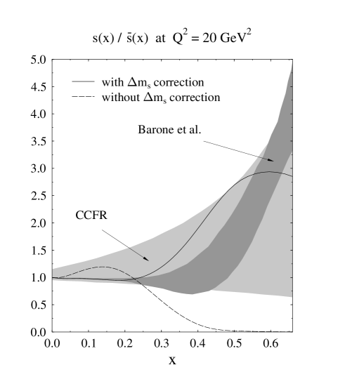
Figure 10: The theoretical predictions for the ratio of $s$- and $\bar{s}$-quark distributions at $Q^{2}=20\,\mbox{GeV}^{2}$ in comparison with the results of CCFR analysis CCFR96 and of Barone et al’s global fit BPZ00 . The meaning of the curves are the same as in Fig. 9

This tendency is more clearly seen in the ratio of $s(x)$ and $\bar{s}(x)$ at $Q^{2}=20\mbox{GeV}^{2}$. In Fig. 10, the solid and dashed curves are the predictions of the SU(3) CQSM with and without the $\Delta m_{s}$ corrections, while the thin and thick shaded areas represent the phenomenologically favorable regions for this ratio, respectively obtained by the CCFR group and by Barone et al. One clearly sees that the observed tendency of this ratio is reproduced (at least qualitatively) only after including the SU(3) symmetry breaking effects.

Now, turning to the spin-dependent distribution functions, the quality of the presently available semi-inclusive data is rather poor, so that the analyses are mainly limited to the inclusive DIS data alone. (There exist some combined analyses of inclusive and semi-inclusive polarized DIS data MY00 ,FS00 ,BB02 .) This forces them to introduce several simplifying assumptions in the fittings. For instance, many previous analyses have used the apparently groundless assumption of a flavor-symmetric polarized sea, i.e. $\Delta\bar{u}(x)=\Delta\bar{d}(x)=\Delta\bar{s}(x)$ GS96 . Another analysis assumed that $\Delta q_{3}(x)=c\,\Delta q_{8}(x)$ with $c$ being a constant. Probably, the most ambitious analyses free from these ad hoc assumptions on the sea-quark distributions are those of Leader, Sidorov and Stamenov (LSS) LSS00 . (See also Ref. GRDV01 .) We recall that they also investigated the sensitivity of their fit to the size of the SU(3) symmetry breaking effect. (Although they did not take account of the possibility that $\Delta s(x)\neq\Delta\bar{s}(x)$, this simplification is harmless, because only the combination $\Delta s(x)+\Delta\bar{s}(x)$ appears in their analyses of DIS data.)

To compare the theoretical distributions of the SU(3) CQSM with the LSS fits given at $Q^{2}=1\mbox{GeV}^{2}$, we must consider the fact that their analyses are carried out in the so-called JET scheme (or the chirally invariant factorization scheme). To take account of this, we start with the theoretical distribution functions $\Delta u(x),\Delta\bar{u}(x),\Delta d(x),\Delta\bar{d}(x),\Delta s(x)$ and $\Delta\bar{s}(x)$, which are taken as the initial scale distribution functions given at $Q^{2}_{ini}=0.30\mbox{GeV}^{2}$. Under the assumption that $\Delta g(x)=0$ at this initial energy scale, we solve the DGLAP equation in the standard $\overline{MS}$ scheme with the gauge-invariant factorization scheme to obtain the distributions at $Q^{2}=1\mbox{GeV}^{2}$. The corresponding distribution functions in the JET scheme are then obtained by the transformation

$$\Delta\Sigma(x.Q^{2})_{JET} = \Delta\Sigma(x.Q^{2})_{\overline{MS}}+\frac{\alpha_{s}(Q^{2})}{\pi}N_{f}(1-x)\otimes\Delta g(x.Q^{2})_{\overline{MS}},$$ (12)

$$\Delta g(x.Q^{2})_{JET} = \Delta g(x.Q^{2})_{\bar{MS}},$$ (13)

with $\Delta\Sigma(x.Q^{2})=\sum^{N_{f}}_{i=1}(\Delta q_{i}(x.Q^{2})+\Delta\bar{q}_{i}(x.Q^{2}))$ being the flavor-singlet quark polarization.

Now we show in Fig. 11 the theoretical distributions $x(\Delta u(x)+\Delta\bar{u}(x)),x(\Delta d(x)+\Delta\bar{d}(x))$, $x(\Delta s(x)+\Delta\bar{s}(x))$ and $\Delta g(x)$ at $Q^{2}=1\mbox{GeV}^{2}$ in comparison with the corresponding LSS fits. The solid and dashed curves in these four figures are respectively the predictions of the SU(3) CQSM obtained with and without the $\Delta m_{s}$ corrections. To estimate the sensitivity of the fit to the SU(3) symmetry breaking effects, Leader et al. performed their fit by varying the value of axial charge $a_{8}$ from its SU(3) symmetric value $0.58$ within the range $0.40\leq a_{8}\leq 0.86$. They found that the value of $\chi^{2}$-fit to the presently available DIS data are practically insensitive to the variation of $a_{8}$, which in turn means that $a_{8}$ cannot be determined from the existing DIS data. Consequently, the distributions $x[\Delta u(x)+\Delta\bar{u}(x)]$ and $x[\Delta d(x)+\Delta\bar{d}(x)]$ are insensitive to the SU(3) symmetry breaking effects and can be determined with little uncertainties. This is also confirmed by our theoretical analysis. In Fig. 11(a) and Fig. 11(b), the solid and dashed curves are the predictions of the SU(3) CQSM for the distributions $x[\Delta u(x)+\Delta\bar{u}(x)]$ and $x[\Delta d(x)+\Delta\bar{d}(x)]$ respectively obtained with and without the $\Delta m_{s}$ corrections. One confirms that they are nearly degenerate and that they reproduce well the results of LSS fit. On the other hand, the distributions of the strange quarks and the gluons are very sensitive to the variation of the axial charge $a_{8}$, so that it brings about large uncertainties for these distributions in the LSS fit as illustrated by the shaded regions in Fig. 11(c) and Fig. 11(d). The feature is again consistent with our theoretical analysis at least for the polarized strange-quark distributions. In fact, the SU(3) CQSM predicts that $x[\Delta s(x)+\Delta\bar{s}(x)]$ is large and negative but the $\Delta m_{s}$ correction reduces its magnitude by a factor of about $0.6$.

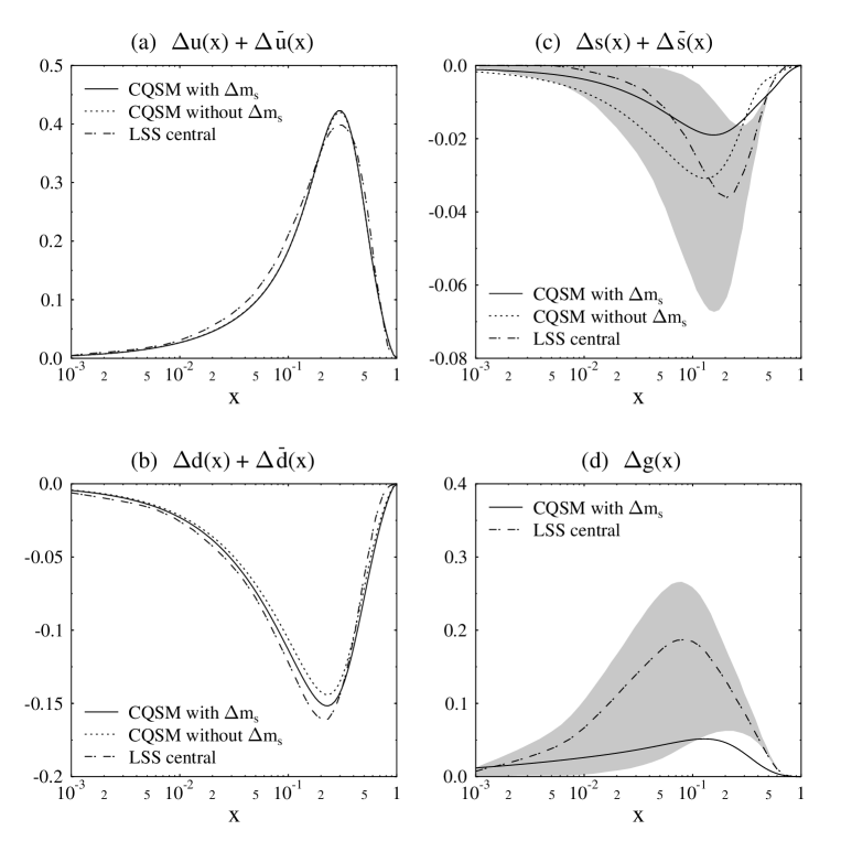
Figure 11: The theoretical distribution functions (a) $x(\Delta u(x)+\Delta\bar{u}(x))$, (b) $x(\Delta d(x)+\Delta\bar{d}(x))$, (b) $x(\Delta s(x)+\Delta\bar{s}(x))$, and (d) $xg(x)$ at $Q^{2}=1\,\mbox{GeV}^{2}$, in comparison with the corresponding LSS fits in the JET scheme LSS00 . Here, the solid and dotted curves are the predictions of the SU(3) CQSM with and without $\Delta m_{s}$ corrections, while the central fit by LSS analyses are represented by the dash-dotted curves. The large uncertainties for the strange-quark distribution as well as the gluon distribution in the LSS fits are illustrated by the shaded areas.

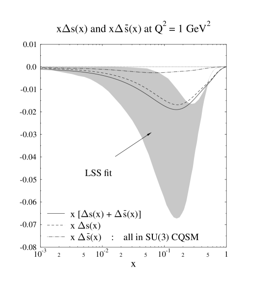
Figure 12: The theoretical prediction of the SU(3) CQSM for the separate contributions of $s$- and $\bar{s}$-quarks to the longitudinally polarized distribution functions $x[\Delta s(x)+\Delta\bar{s}(x)]$ in comparison with the LSS fit LSS00 .

A noteworthy feature of the theoretical predictions of the SU(3) CQSM is that the negative polarization of strange sea comes almost solely from $\Delta s(x)$, while $\Delta\bar{s}(x)$ is nearly zero. This is illustrated in Fig. 12. The predicted sizable particle-antiparticle asymmetry of the polarized strange sea can be verified only by the near future experiments beyond the totally inclusive DIS scatterings such as the semi-inclusive DIS processes, the neutrino reactions, etc.

Figure 13: The flavor nonsinglet and single combinations of the longitudinally polarized distribution functions and their ratio at $Q^{2}=1\,\mbox{GeV}^{2}$ in the JET scheme : (a) $\Delta q_{3}(x),\Delta q_{8}(x)$, and $\Delta q_{0}(x)$, and (b) $\Delta q_{3}(x)/\Delta q_{8}(x)$. In the right panel, the solid and dashed curves are the predictions of the SU(3) CQSM with and without $\Delta m_{s}$ corrections, whereas the dash-dotted curve stands for the corresponding LSS fit.

From the theoretical viewpoint, it is interesting to see the particular linear combinations of the distributions $\Delta u(x)+\Delta\bar{u}(x),\Delta d(x)+\Delta\bar{d}(x)$ and $\Delta s(x)+\Delta\bar{s}(x)$ given by

$$\Delta q_{0}(x) = \Delta u(x)+\Delta\bar{u}(x)+\Delta d(x)+\Delta\bar{d}(x)+\Delta s(x)+\Delta\bar{s}(x),$$ (14)

$$\Delta q_{3}(x) = \Delta u(x)+\Delta\bar{u}(x)-\Delta d(x)-\Delta\bar{d}(x),$$ (15)

$$\Delta q_{8}(x) = \Delta u(x)+\Delta\bar{u}(x)+\Delta d(x)+\Delta\bar{d}(x)-2\,[\Delta s(x)+\Delta\bar{s}(x)].$$ (16)

We show in Fig. 13(a) the predictions of the SU(3) CQSM for these densities at $Q^{2}=1\mbox{GeV}^{2}$ in the JET scheme. One clearly sees that $\Delta q_{0}(x)$ is negative in the smaller $x$ region. One can also convince that the polarized strange quark densities given by

$$\Delta s(x)+\Delta\bar{s}(x)=\frac{1}{3}\,[\Delta q_{0}(x)-\Delta q_{8}(x)],$$ (17)

is certainly negative for all range of $x$. Of special interest here is the difference or the ratio of $\Delta q_{3}(x)$ and $\Delta q_{8}(x)$, since, as already pointed out, some previous phenomenological analyses assume $\Delta q_{3}(x)/\Delta q_{8}(x)=$ constant with no justification. The solid and dashed curves in Fig. 13(b) are the predictions of the SU(3) CQSM for this ratio, respectively obtained with and without $\Delta m_{s}$ corrections, while dash-dotted curves is the corresponding result of LSS fit. After including the SU(3) symmetry breaking effects, one can say that the theory reproduces the qualitative behavior of the LSS fit for this ratio.

Through the analyses so far, we have shown that the flavor SU(3) CQSM can give unique and interesting predictions for both of the unpolarized and the longitudinally polarized strange quark distributions in the nucleon, all of which seems to be qualitatively consistent with the existing phenomenological information for strange quark distributions. A natural question here is whether or not it is realistic enough as the flavor SU(2) CQSM has been proved so. (We recall that the SU(2) CQSM reproduces almost all the qualitatively noticeable features of the presently available DIS data.) Which is more realistic model of the nucleon, the SU(2) CQSM or the SU(3) one? Naturally, at least concerning one particular aspect, i.e. the problem of hidden strange-quark excitations in the nucleon, the SU(3) model is superior to the SU(2) model, since the strange quark excitations in the nucleon can be treated only in the former model. The question is then reduced to which model gives more realistic descriptions for the $u,d$-flavor dominated observables, which have been the objects of studies of the SU(2) CQSM. To answer this question, we try to reanalyze several interesting observables, which we have investigated before in the SU(2) CQSM, here within the framework of the flavor SU(3) CQSM.

Figure 14: The theoretical predictions for the proton, neutron, and deuteron spin structure functions $g_{1}^{p}(x),g_{1}^{n}(x)$, and $g_{1}^{d}(x)$ at $Q^{2}=5\,\mbox{GeV}^{2}$ in comparison with the corresponding SLAC and SMC data. The solid and dashed curves in these figures respectively stand for the predictions of the SU(3) CQSM and those of the SU(2) CQSM. The black circles in (a) and (b) are the E143 E143 and the E154 data E154 , while the diamonds, the circles and the squares in (c) represent the E143 E143 , the E155 E155 and the SMC data SMC98 .

At this opportunity, the calculation in the SU(2) model were redone, because there is a little change in the theoretical treatment of the $O(\Omega^{1})$ contribution to the longitudinally polarized distribution functions as was explained in the previous section. First, in Fig. 14, we show the theoretical predictions of the SU(3) and SU(2) CQSM for the longitudinally polarized structure functions of the proton, the neutron and the deuteron in comparison with the corresponding EMC and SMC data at $Q^{2}=5\mbox{GeV}^{2}$. Here, the solid and dashed curves are the predictions of the SU(3) and SU(2) CQSM, respectively. The black circles in Fig. 14(a) are E143 data, whereas those in Fig. 14(b) are E154 data E154 . On the other hand, the black circles, white circles and white squares in Fig. 14(c) and Fig. 14(d) correspond to the E143 E143 , E155 E155 and SMC data SMC98 , respectively. Comparing the predictions of the two versions of the CQSM, one notices two features. First, the magnitudes of $g_{1}^{p}(x)$ and $g_{1}^{n}(x)$ are reduced a little when going from the SU(2) model to the SU(3) one. As we will discuss shortly, this feature can be understood as a reduction of the isovector axial charge in the SU(3) CQSM. Another feature is that the small $x$ behavior of the deuteron structure function (the flavor singlet one) becomes slightly worse in the SU(3) model. (This is due to the SU(3) symmetry breaking effects.) These differences between the predictions of the SU(3) CQSM and the SU(2) one are very small, however. Considering the qualitative nature of our model as an effective low energy theory of QCD, we may be allowed to say that both models reproduces the experimental data fairly well.

Table 1: The predictions of the SU(3) and SU(2) CQSM for the axial charges, the quark polarization $\Delta q\equiv\int_{0}^{1}\,[\Delta q(x)+\Delta\bar{q}(x)]\,dx$ of each flavor, and the basic coupling constant of SU(3), in comparison with phenomenological information. Here, the experimental values for $g_{A}^{(3)},g_{A}^{(8)},F,D$ and $F/D$ are from CR93 , while $\Delta u,\Delta d,\Delta s$ and $g_{A}^{(0)}$ corresponds to the values at $Q^{2}=10\,\mbox{GeV}^{2}$ given in EK95 .

	SU(2) CQSM	SU(3) CQSM	Experiment
$g_{A}^{(3)}$	1.41	1.20	1.257 $\pm$ 0.016
$g_{A}^{(8)}$	—	0.59	0.579 $\pm$ 0.031
$g_{A}^{(0)}$	0.35	0.36	0.31 $\pm$ 0.07
$\Delta u$	0.88	0.82	0.82 $\pm$ 0.03
$\Delta d$	-0.53	-0.38	-0.44 $\pm$ 0.03
$\Delta s$	0	-0.08	-0.11 $\pm$ 0.03
$F$	—	0.45	0.459 $\pm$ 0.008
$D$	—	0.76	0.798 $\pm$ 0.008
$F/D$	—	0.59	0.575 $\pm$ 0.016

As mentioned above, the reduction of the magnitudes of $g_{1}^{p}(x)$ and $g_{1}^{n}(x)$ in the SU(3) CQSM can be traced back to the change of the isovector charge, which is related to the first moment of $g_{1}^{p}(x)-g_{1}^{n}(x)$. We show in Table 1 the predictions of the SU(3) and SU(2) CQSM for the flavor nonsinglet as well as flavor singlet axial charges, the quark polarization of each flavor defined as $\Delta q=\int_{0}^{1}\,[\Delta q(x)+\Delta\bar{q}(x)]\,dx$, in comparison with some phenomenological information. One sees that, aside from the addition of the strange quark degrees of freedom, a main change when going from the SU(3) model to the SU(2) one is a decrease of isovector axial charge $g_{A}^{(3)}$, while the flavor singlet axial charge $g_{A}^{(0)}$ is almost unchanged. Corresponding to this reduction of $g_{A}^{(3)}$, the magnitudes of $\Delta u$ and $\Delta d$ are both reduced a little. Also shown in this table is the fundamental coupling constants $F$ and $G$ in the flavor SU(3) scheme as well as their ratio. They are all qualitatively consistent with the phenomenological information. Interestingly, the predicted ratio $F/D$ is very close to that of the naive SU(6) model, i.e. $3/5$, even though such dynamical symmetry is not far from being justified in our theoretical framework.

Next, we go back to the spin-independent observables. The solid and dashed curves in Fig. 15(a) stand for the predictions of the SU(3) and SU(2) CQSM for the difference $F^{p}_{2}(x)-F^{n}_{2}(x)$ of the proton and neutron structure function $F_{2}(x)$, in comparison with the corresponding NMC data at $Q^{2}=4\mbox{GeV}^{2}$. One the other hand, the solid and dashed curves in Fig. 15(b) are the predictions of the SU(3) and SU(2) CQSM for the ratio $F^{n}_{2}(x)/F^{p}_{2}(x)$ in comparison with the NMC data. One confirms that these difference and the ratio functions are rather insensitive to the flavor SU(3) generalization of the model and that the success of the SU(2) CQSM is basically taken over by the SU(3) model.

Figure 15: The theoretical predictions of the two versions of the CQSM for $F_{2}^{p}(x)-F_{2}^{n}(x)$ and $F_{2}^{n}(x)/F_{2}^{p}(x)$ at $Q^{2}=4\,\mbox{GeV}^{2}$ are compared with the NMC data given at the corresponding energy scale NMC91 .

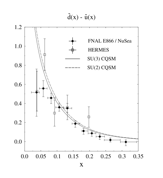
Figure 16: The theoretical predictions of the SU(3) and SU(2) CQSM for the unpolarized antiquark distribution $\bar{d}(x)-\bar{u}(x)$ at $Q^{2}=54\,\mbox{GeV}^{2}$ in comparison with the HERMES HERMES and E866 data E866 .

In Fig. 16, the theoretical predictions of both models for the sea-quark distribution $\bar{d}(x)-\bar{u}(x)$ is compared with the corresponding E866 data at $Q^{2}=54\mbox{GeV}^{2}$ E866 and with HERMES data at $Q^{2}=4\mbox{GeV}^{2}$ HERMES , for reference. The isospin asymmetry of the sea-quark distributions or the magnitude of $\bar{d}(x)-\bar{u}(x)$ turns out to become a little smaller in the SU(3) model than in the SU(2) model, although the change is fairly small.

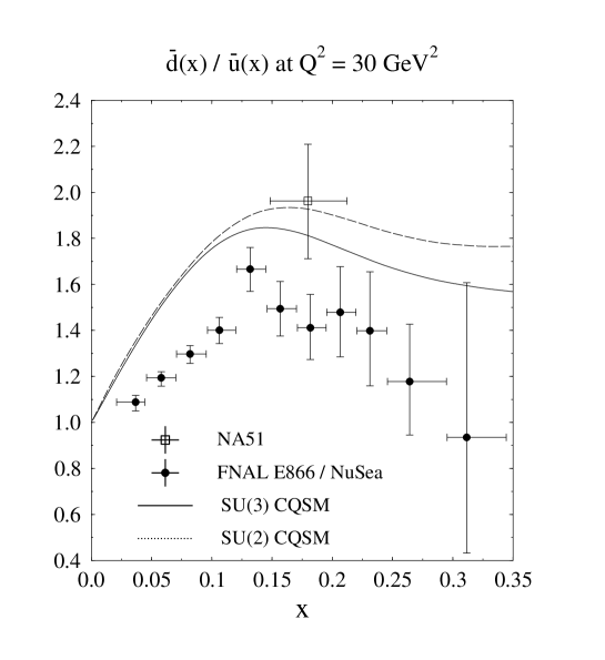
Figure 17: The theoretical predictions of the SU(3) and SU(2) CQSM for the ratio $\bar{d}(x)/\bar{u}(x)$ in the proton as a function of $x$ in comparison with the result of E866 analysis E866 . Also shown is the result from NA51 NA51 , plotted as an open box.

Figure 18: The isospin asymmetries of the light-flavor sea-quark distribution functions evaluated at $Q^{2}=0.88\,\mbox{GeV}^{2}$ in the standard $\overline{MS}$ factorization scheme with gauge invariant regularization. The left figure shows the unpolarized distribution $x[\bar{d}(x)-\bar{u}(x)]$, while the right figure represents the longitudinally polarized one $x[\Delta\bar{u}(x)-\Delta\bar{d}(x)]$. In both figures, the solid and dash-dotted curves are the predictions of the SU(3) CQSM with and without $\Delta m_{s}$ corrections, whereas the dotted curves are those of the SU(2) CQSM. Bhalerao’s semi-theoretical predictions are also shown for comparison B01 .

Next, in Fig. 17, the theoretical predictions for the ratio $\bar{d}(x)/\bar{u}(x)$ at $Q^{2}=30\,\mbox{GeV}^{2}$ are compared with the corresponding E866 data as well as the old NA51 data. This ratio turns out to be a little sensitive to the flavor SU(3) generalization of the model. It is found that the SU(3) version of the CQSM well reproduces the qualitative tendency of the E866 data for this ratio, although the magnitude itself is a little overestimated. To reveal the reason of this overestimation, it may be interesting to compare the magnitudes of quark and antiquark distributions themselves. Shown in Fig. 19 are the predictions of the SU(3) CQSM for the unpolarized quark and antiquark distribution functions with each flavor at $Q^{2}=20\,\mbox{GeV}^{2}$. Of special interest here are the magnitudes of $\bar{u}(x),\bar{d}(x)$ and $\bar{s}(x)$. The model predicts that

$$\bar{d}(x)\ >\ \bar{s}(x)\ >\ \bar{u}(x),$$ (18)

while the standard MRST MRST98 or CTEQ fit CTEQ00 says that

$$\bar{d}(x)\ >\ \bar{u}(x)\ >\ \bar{s}(x).$$ (19)

Undoubtedly, the magnitudes of $\bar{u}$-distribution as compared with the other two flavors seems to be underestimated a little too much by some reason.

Figure 19: The theoretical predictions of the SU(3) CQSM for the unpolarized quark and antiquark distribution functions with each flavor at the energy scale of $Q^{2}=20\,\mbox{GeV}^{2}$.

As repeatedly emphasized, a quite unique feature of the SU(2) CQSM is that it predicts sizably large isospin asymmetry not only for the unpolarized sea-quark distributions but also for the longitudinally polarized ones. A natural question is what the predictions of the flavor SU(3) CQSM is like. We have already shown that the predictions of these two models are not largely different for the isospin asymmetry of the unpolarized seas, for instance, for $\bar{d}(x)-\bar{u}(x)$. To confirm it again but here in comparison with the case of polarized distributions, we show in Fig. 18 the theoretical predictions for $\bar{d}(x)-\bar{u}(x)$ evaluated at $Q^{2}=0.88\mbox{GeV}^{2}$ in comparison with Bhalerao’s semi-theoretical prediction for reference B01 . The solid and dashed-dotted curves in Fig. 18(a) are the predictions of the SU(3) CQSM obtained with and without the $\Delta m_{s}$ corrections, while the dotted curve is the prediction of the SU(2) CQSM. We recall that Bhalerao’s prediction shown by the dotted curve is obtained based on what-he-call the statistical quark model, which is based on some statistical assumptions on the parton distributions while introducing several experimental information. As one can see, all the four curves are more or less degenerate and they are all qualitatively consistent with the magnitude of isospin asymmetry of $\bar{d}$-sea and $\bar{u}$-sea observed by the NMC measurement. On the other hand, Fig. 18(b) shows the similar analysis for the longitudinally polarized sea-quark distributions $\Delta\bar{u}(x)-\Delta\bar{d}(x)$. The meaning of the curves are all similar as in Fig. 18(a). One finds that the magnitude of $\Delta\bar{u}(x)-\Delta\bar{d}(x)$ is fairly sensitive to the flavor SU(3) generalization of the CQSM, or more precisely, to the difference between the dynamical assumptions of the two models. (This provides us with one of the few exceptions to our earlier statement that $u,d$-flavor dominated observables are generally insensitive to it.) The sign of $\Delta\bar{u}(x)-\Delta\bar{d}(x)$ remains definitely positive but its magnitude is reduced by nearly a factor of 2 when going from the SU(2) model to the SU(3) model the chiral limit ($\Delta m_{s}=0$). As was conjectured in W02 , the inclusion of the SU(3) symmetry breaking corrections partially cancels this reduction and works to pull back the prediction of the SU(3) model toward that of the SU(2) model. Still, the final prediction of the SU(3) CQSM is fairly small as compared with that of the SU(2) one although it is not extremely far from the prediction of Bhalerao’s statistical model B01 .

One may be also interested in the signs and the relative order of the absolute magnitudes of $\Delta\bar{u}(x),\Delta\bar{d}(x)$ and $\Delta\bar{s}(x)$ themselves. We show in Fig. 20 the theoretical predictions of the SU(3) CQSM for the longitudinally polarized quark and antiquark distributions with each flavor at the energy scale of $Q^{2}=0.88\,\mbox{GeV}^{2}$. In addition to that the model reproduces the well-established fact $\Delta u(x)>0$ and $\Delta d(x)<0$, it also predicts that $\Delta\bar{u}(x)>0,\Delta\bar{d}(x)<0$ and $\Delta\bar{s}(x)<0$ with

$$|\Delta\bar{d}(x)|\ >\ |\Delta\bar{u}(x)|\ >\ |\Delta\bar{s}(x)|.$$ (20)

We point out that these predictions of the SU(3) CQSM are qualitatively consistent with those of Bhalerao’s statistical quark model except for the fact that he assumes $\Delta s(x)=\Delta\bar{s}(x)$, while the SU(3) CQSM indicates that

$$|\Delta s(x)|\ \gg\ |\Delta\bar{s}(x)|.$$ (21)

Figure 20: The theoretical predictions of the SU(3) CQSM for the longitudinally polarized quark and antiquark distribution functions with each flavor at the scale of $Q^{2}=0.88\,\mbox{GeV}^{2}$.

Summarizing the predictions of the two versions of the CQSM for the light-flavor sea-quark asymmetry, both turn out to give equally good explanation for the shape and magnitude of spin-independent distribution $\bar{d}(x)-\bar{u}(x)$. The situation is a little different for the longitudinally polarized sea-quark distributions. Although the sign of $\Delta\bar{u}(x)-\Delta\bar{d}(x)$ is definitely positive in both models, the SU(2) CQSM predicts that

$$|\bar{u}(x)-\bar{d}(x)|\ <\ |\Delta\bar{u}(x)-\Delta\bar{d}(x)|,$$ (22)

while the SU(3) model gives

$$|\bar{u}(x)-\bar{d}(x)|\ \simeq\ |\Delta\bar{u}(x)-\Delta\bar{d}(x)|,$$ (23)

or $|\Delta\bar{u}(x)-\Delta\bar{d}(x)|$ is slightly small than $|\bar{u}(x)-\bar{d}(x)|$. Still, the sizably large isospin asymmetry of the spin-dependent sea-quark distributions is a common feature of the two versions of the CQSM. (It is interesting to remember that large flavor and spin asymmetry of the nucleon sea is also predicted by the instanton model DK93 ,DKZ93 .) We think that this fact is worthy of special mention. The reason becomes clear if one compares the predictions of the CQSM with those of the naive meson cloud convolution model. As is widely known, the NMC observation $\bar{d}(x)-\bar{u}(x)>0$ in the proton can be explained equally well by the CQSM and by the meson cloud model K98 ,GP01 ,Ram97 . A simple intuitive argument, however, indicates that the latter model would generally predict both of $\Delta\bar{u}(x)$ and $\Delta\bar{d}(x)$ is small. This is because the lightest meson, i.e. the pion has no spin and that the effect of heavier meson is expected to be less important. Actually, the situation seems a little more complicated. In a recent paper, Kumano and Miyama estimated the contribution of $\rho$-meson to the asymmetry $\Delta\bar{u}(x)-\Delta\bar{d}(x)$ and found that it is slightly negative KM02 . On the other hand, Fries et al. argued that a large positive $\Delta\bar{u}(x)-\Delta\bar{d}(x)$, as obtained in the CQSM, can be obtained from $\pi N$-$\sigma N$ interference-type contributions in the meson cloud picture FSW02 . Undoubtedly, for drawing a definite conclusion within the framework of the meson cloud model, more exhaustive studies of possibly important Feynman diagrams are necessary. This should be contrasted with the prediction of the CQSM. Since there is little arbitrariness in its theoretical framework, its prediction once given is one and only in nature and cannot be easily modified. Both of the CQSM and the meson cloud convolution model give equally nice explanation for the novel isospin asymmetry for the unpolarized sea-quark distributions, so that one might have naively thought that they are two similar models containing basically the same physics. In fact, a commonly important ingredients of the two models are the Nambu-Goldstone pions resulting from the spontaneous chiral symmetry breaking of QCD vacuum. However, a lesson learned from the above consideration of the isospin asymmetry for the spin-dependent sea-quark distributions is that it is not necessarily true. An interesting question is what makes a marked difference between these two models. In our opinion, it is a strong correlation between spin and isospin quantum numbers embedded in the basic dynamical assumption of the CQSM, i.e. the hedgehog ansatz. We recall that we have long known one example in which the difference of these two models makes more profound effect W89 ,W90 ,WY91 ,WW00B . It is just the problem of quark spin fraction of the nucleon. Is there any simple and convincing explanation of this nucleon spin puzzle within the framework of the meson cloud model? The answer is no, to our knowledge. On the other hand, assuming that the dynamical assumption of the CQSM is justified in nature, it gives quite a natural answer to the question why the quark spin fraction of the nucleon is so small. In fact, according to this model, a nucleon is a bound state of quarks and antiquarks moving in the rotating mean-field of hedgehog shape. Because of the collective rotational motion, it happens that a sizable amount ($\sim 65\%$) of the total nucleon spin is carried by the orbital angular momentum of quark and antiquark fields. We conjecture that the cause of the simultaneous large violation of the isospin asymmetry for both the spin-independent and spin-dependent sea-quark distributions can also be traced back to the strong spin-isospin correlation generated by the formation of the hedgehog mean field.

IV Summary and Conclusion

In summary, several theoretical predictions are given for the light-flavor quark and antiquark distribution functions in the nucleon on the basis of the flavor SU(3) CQSM. Its basic lagrangian is a straightforward generalization of the corresponding SU(2) model except for the presence of sizably large SU(3) symmetry breaking term, which comes from the appreciable mass difference $\Delta m_{s}$ between the $s$-quark and the $u,d$-quarks. As explained in the text, this SU(3) symmetry breaking effect is treated by using a perturbation theory in the mass parameter $\Delta m_{s}$. We have shown that the SU(3) CQSM can give several unique predictions for the strange and antistrange quark distributions in the nucleon while maintaining the success previously obtained in the flavor SU(2) version of the CQSM for $u,d$-flavor dominated observables. For instance, it predicts a sizable amount of particle-antiparticle asymmetry for the strange-quark distributions. Its predictions for the distributions $s(x)-\bar{s}(x)$ and $s(x)/\bar{s}(x)$ at $Q^{2}=20\,\mbox{GeV}^{2}$ are shown to be consistent with the corresponding phenomenological information given by Barone et al. and by CCFR group at least qualitatively. As expected, the magnitudes of $s(x)$ and $\bar{s}(x)$ turn out to be very sensitive to the SU(3) symmetry breaking effects. We showed that the theoretical predictions for $x\bar{s}(x)$ and $x\bar{s}(x)$ at $Q^{2}=4\,\mbox{GeV}^{2}$ and $Q^{2}=20\,\mbox{GeV}^{2}$ are qualitatively consistent with the CCFR data after taking account of the SU(3) symmetry breaking effects. The particle-antiparticle asymmetry of the strange quark distributions are even more profound for the spin-dependent distributions than for the unpolarized distributions. Our theoretical analysis strongly indicates that the negative (spin) polarization of the strange quarks, i.e. the fact that $\Delta s(x)+\Delta\bar{s}(x)<0$, as suggested by the LSS fit as well as many other phenomenological analyses, comes almost solely from the $s$-quark and the polarization of $\bar{s}$-quark is very small. The model gives interesting predictions also for the isospin asymmetry of the $\bar{u}$- and $\bar{d}$-quark distributions. We had already known that the flavor SU(2) CQSM gives a natural explanation of the NMC observation, i.e. the excess of $\bar{d}$-sea over the $\bar{u}$-sea in the proton. In the present investigation, we have confirmed that this favorable aspect of the SU(2) CQSM is just taken over by the SU(3) CQSM and that they in fact give nearly the same predictions for the magnitude of the asymmetry $\bar{d}(x)-\bar{u}(x)$. On the other hand, we find that the predictions of the two models for the isospin asymmetry of the longitudinally polarized sea-quark distributions are a little different. Both models predicts that $\Delta\bar{u}(x)-\Delta\bar{d}(x)>0$, but the magnitude of asymmetry is reduced by a factor of about 0.6 when going from the SU(2) model to the SU(3) one. Still, a sizably large isospin asymmetry of the spin-dependent sea-quark distributions is a common prediction of both versions of the CQSM, and it should be compared with the unsettled situation in the meson-cloud convolution models. In our opinion, the physical origin of the simultaneous violation of the isospin symmetry for the spin-independent and spin-dependent sea-quark distributions may be traced back to the strong correlation between spin and isospin embedded in the hedgehog symmetry of soliton solution expected to be realized in the large $N_{c}$ limit of QCD. What should be emphasized here is another consequence of the hedgehog symmetry embedded in the CQSM. It has long been recognized that, according to this model, only about $35\,\%$ of the total nucleon spin is due to the intrinsic quark spin and the remaining $65\,\%$ is borne by the orbital angular momentum of quark and antiquark fields. We emphasize that this is a natural consequence of the nucleon picture of this model, i.e. “rotating hedgehog”. Unfortunately, unresolved role of gluon fields, especially the role of $U_{A}(1)$ anomaly makes it difficult to draw a definite conclusion on this interesting but mysterious problem. In this respect, more thorough study of simpler problem, i.e. the possible isospin asymmetry of longitudinally polarized sea-quark distributions may be of some help to test the validity of the basic idea of the soliton picture of the nucleon. At any rate, an important lesson learned from our whole analyses is that the spin and flavor dependencies of antiquark distributions in the nucleon are very sensitive to the nonperturbative dynamics of QCD. To reveal this interesting aspect of baryon structures, it is absolutely necessary to carry out flavor and valence plus sea quark decompositions of the parton distribution functions. We hope that this expectation will soon be fulfilled by various types of semi-inclusive DIS scatterings as well as neutrino-induced reactions planned in the near future.

- [1] M. Glück, E. Reya, and A. Vogt. Z. Phys., C67:433, 1995.
- [2] M. Glück, E. Reya, M. Stratmann, and W. Vogelsang. Phys. Rev., D53:4775, 1996.
- [3] NMC Collaboration : P. Amaudruz et al. Phys. Rev. Lett., 66:2712, 1991.
- [4] D.I. Diakonov, V.Yu. Petrov, and P.V. Pobylitsa. Nucl. Phys., B306:809, 1988.
- [5] M. Wakamatsu and H. Yoshiki. Nucl. Phys., A524:561, 1991.
- [6] M. Wakamatsu. Prog. Theor. Phys. Suppl., 109:115, 1992.
- [7] Chr.V. Christov, A. Blotz, H.-C. Kim, P.V. Pobylitsa, T. Watabe, Th. Meissner, E. Ruiz Arriola, and K. Goeke. Prog. Part. Nucl. Phys., 37:91, 1996.
- [8] R. Alkofer, H. Reinhardt, and H. Weigel. Phys. Rep., 265:139, 1996.
- [9] D.I. Diakonov and V.Yu. Petrov. At the frontier of particle physics, Vol.1. National Academy Press, 2001.
- [10] D.I. Diakonov, V.Yu. Petrov, P.V. Pobylitsa, M.V. Polyakov, and C. Weiss. Nucl. Phys., B480:341, 1996.
- [11] D.I. Diakonov, V.Yu. Petrov, P.V. Pobylitsa, M.V. Polyakov, and C. Weiss. Phys. Rev., D56:4069, 1997.
- [12] M. Wakamatsu and T. Kubota. Phys. Rev., D56:4069, 1998.
- [13] M. Wakamatsu and T. Kubota. Phys. Rev., D60:034020, 1999.
- [14] M. Wakamatsu. Phys. Rev., D44:R2631, 1991.
- [15] M. Wakamatsu. Phys. Lett., B269:394, 1991.
- [16] M. Wakamatsu. Phys. Rev., D46:3762, 1992.
- [17] P.V. Pobylitsa, M.V. Polyakov, K. Goeke, T. Watabe, and C. Weiss. Phys. Rev., D59:034024, 1999.
- [18] M. Wakamatsu and T. Watabe. Phys. Rev., D62:017506, 2000.
- [19] M. Wakamatsu and T. Watabe. Phys. Rev., D62:054009, 2000.
- [20] B. Dressler, K. Goeke, M.V. Polyakov, and C. Weiss. Eur. Phys. J., C14:147, 2000.
- [21] M. Wakamatsu. Prog. Theor. Phys., 107:1037, 2002.
- [22] H. Weigel, R. Alkofer, and H. Reinhardt. Nucl. Phys., B387:638, 1992.
- [23] A. Blotz, D.I. Diakonov, K. Goeke, N.W. Park, V.Yu. Petrov, and P.V. Pobylitsa. Nucl. Phys., A555:765, 1993.
- [24] E. Guadanini. Nucl. Phys., B336:35, 1984.
- [25] P.O. Mazur, M.A. Nowak, and M. Praszałowicz. Phys. Lett., 147B:137, 1984.
- [26] M. Wakamatsu and T. Watabe. Phys. Lett., B312:184, 1993.
- [27] Chr.V. Christov, A. Blotz, K. Goeke, P. Pobylitsa, V.Yu. Petrov, M. Wakamatsu, and T. Watabe. Phys. Lett., B325:467, 1994.
- [28] J. Schechter and H. Weigel. Mod. Phys. Lett., A10:885, 1995.
- [29] J. Schechter andH¿ Weigel. Phys. Rev., D51:6296, 1995.
- [30] M. Wakamatsu. Phys. Lett., B349:204, 1995.
- [31] M. Wakamatsu. Prog. Theor. Phys., 95:143, 1996.
- [32] Chr. V. Christov, K. Goeke, and P.V. Pobylitsa. Phys. Rev., C52:425, 1995.
- [33] R. Alkofer and H. Weigel. Phys. Lett., B319:1, 1993.
- [34] M. Praszałowicz, T. Watabe, and K. Goeke. Nucl. Phys., A647:49, 1999.
- [35] H. Weigel, E. Ruiz Arriola, and L. Gamberg. Nucl. Phys., B560:383, 1999.
- [36] T. Kubota, M. Wakamatsu, and T. Watabe. Phys. Rev., D60:014016, 1999.
- [37] J. Gasser, H. Leutwyler, and M.E. Sainio. Phys. Lett., B253:252, 1991.
- [38] M. Miyama and S. Kumano. Comput. Phys. Commun., 94:185, 1996.
- [39] M. Hirai, S. Kumano, and M. Miyama. Comput. Phys. Commun., 108:38, 1998.
- [40] M. Hirai, S Kumano, and M. Miyama. Comput. Phys. Commun., 111:150, 1998.
- [41] M. Burkardt, X. Ji, and F. Yuan. Phys. Lett., B545:345, 2002.
- [42] O. Schröder, H. Reinhardt, and H. Weigel. Nucl. Phys., A651:174, 1999.
- [43] O. Schröder, H. Reinhardt, and H. Weigel. Phys. Lett., B439:398, 1998.
- [44] CCFR Collaboration : A. Bazarko et al. Z. Phys., C65:189, 1995.
- [45] S. Brodsky and B. Ma. Phys. Lett., B381:317, 1996.
- [46] A.I. Signal and A.W. Thomas. Phys. Lett., B191:205, 1987.
- [47] V. Barone, C. Pascaud, and F. Zomer. Eur. Phys. J., C12:243, 2000.
- [48] T. Morii and T. Yamanishi. Phys. Rev., D61:057501, 2000.
- [49] D.de Florian and R. Sassot. Phys. Rev., D62:094025, 2000.
- [50] J. Blümlein and H. Böttcher. Nucl. Phys., B636:225, 2002.
- [51] T. Gehrmann and W. Stirling. Phys. Rev., D53:6100, 1996.
- [52] E. Leader, A. Sidorov, and D. Stamenov. Phys. Lett., B488:283, 2000.
- [53] M. Glück, E. Reya, M. Stratmann, and W. Vogelsang. Phys. Rev., D63:094005, 2001.
- [54] E143 Collaboration : K. Abe et al. Phys. Rev., D58:112003, 1998.
- [55] E154 Collaboration : K. Abe et al. Phys. Rev. Lett., 79:26, 1997.
- [56] E155 Collaboration : P.L. Anthony et al. Phys. Lett., B463:339, 1999.
- [57] SMC Collaboration : B. Adeva et al. Phys. Rev., D58:112001, 1998.
- [58] F.E Close and R.G. Roberts. B316:165, 1993.
- [59] J. Ellis and M. Karliner. Phys. Lett., B341:397, 1995.
- [60] HERMES Collaboration : K. Ackerstaff et al. Phys. Rev. Lett., 81:5519, 1998.
- [61] E866 Collaboration : E. A. Hawker et al. Phys. Rev. Lett., 80:3715, 1998.
- [62] A. Baldit et al. Phys. Lett., B332:244, 1994.
- [63] R. Bhalerao. Phys. Rev., C63:025208, 2001.
- [64] A. D. Martin, R.G. Roberts, W.J. Stirling, and R.S. Thorne. Eur. Phys. J., C4:463, 1998.
- [65] CTEQ Collaboration : H. L. Lai et al. Eur. Phys. J., C12:375, 2000.
- [66] A.E. Dorokhov and N.I. Kochelev. Phys. Lett., B304:167, 1993.
- [67] A.E. Dorokhov, N.I. Kochelev, and Yu.A. Zubov. Int. J. Mod. Phys., A8:603, 1993.
- [68] S. Kumano. Phys. Rep., 303:183, 1998.
- [69] G.T. Garvey and J.-C. Peng. Progress in Particle and Nuclear Physics, 47:203, 2001.
- [70] G.P. Ramsey. Prog. Part. Nucl. Phys., 39:599, 1997.
- [71] S. Kumano and M. Miyama. Phys. Rev., D65:034012, 2002.
- [72] R.J. Fries, A. Schäfer, and C. Weiss. hep-ph / 0204060, 2002.
- [73] M. Wakamatsu. Phys. Lett., B232:251, 1989.
- [74] M. Wakamatsu. Phys. Rev., D42:2427, 1990.