NNLL corrections to the angular distribution and to the forward-backward asymmetries in $b\rightarrow X_{s}\ell^{+}\ell^{-}$

Abstract

We present next-to-next-to leading logarithmic (NNLL) results for the double differential decay width $d\Gamma(b\rightarrow X_{s}\ell^{+}\ell^{-})/(d\hat{s}\,d\cos(\theta))$, where $s=\hat{s}\,m_{b}^{2}$ is the invariant mass squared of the lepton pair and $\theta$ is the angle between the momenta of the $b$-quark and the $\ell^{+}$, measured in the rest-frame of the lepton pair. From these results we also derive NNLL results for the lepton forward-backward asymmetries, as these quantities are known to be very sensitive to new physics. While the principal steps in the calculation of the double differential decay width are the same as for $d\Gamma(b\rightarrow X_{s}\ell^{+}\ell^{-})/d\hat{s}$, which is already known to NNLL precision, genuinely new calculations for the combined virtual- and gluon bremsstrahlung corrections associated with the operators $O_{7}$, $O_{9}$ and $O_{10}$ are necessary. In this paper, we neglected certain other bremsstrahlung contributions, which are known to have only a small impact on $d\Gamma(b\rightarrow X_{s}\ell^{+}\ell^{-})/d\hat{s}$. We find that the NNLL corrections drastically reduce the renormalization scale ($\mu$) dependence of the forward-backward asymmetries. In particular, $\hat{s}_{0}$, the position at which the forward-backward asymmetries vanish, is essentially free of uncertainties due to the renormalization scale at NNLL precision. We find $\hat{s}_{0}^{\rm{NNLL}}=0.162\pm 0.005$, where the error is dominated by the uncertainty in $m_{c}/m_{b}$. This is to be compared with $\hat{s}_{0}^{\rm{NLL}}=0.144\pm 0.020$, where the error is dominated by uncertainties due to the choice of $\mu$.

I Introduction

Rare $B$-meson decays are known to be important sources for informations on the standard model (SM) of electroweak and strong interactions and its extensions. Being very sensitive to the actual physics at the scales of several hundred GeV, they can be used to distinguish between different models of fundamental physics and, in particular, to find significant deviations from the SM predictions. Even restricting the consideration to the SM case, these decays can be used to retrieve important information on the properties of the top quark, e.g. to determine the elements $V_{ts}$ and $V_{td}$ of the Cabibbo-Kobayashi-Maskawa (CKM) matrix.

The first measured rare $B$-meson decay was the exclusive channel $B\rightarrow K^{*}\gamma$, observed by the CLEO collaboration in 1992 [1]. It was followed by the observation of the corresponding inclusive mode $B\rightarrow X_{s}\gamma$ [2]. The measured decay rate [2, 3, 4, 5] and the photon energy spectrum [6] for the latter are in good agreement with the predictions of the SM [7, 8, 9, 10, 11, 12, 13]. Thus, these observables are well suited for constraining the SM extensions, such as two-Higgs doublet models [14, 9, 15], left-right symmetric models [16], supersymmetric models [17, 18, 19, 20, 21, 22], etc..

Among the other rare transitions, the inclusive decay $B\rightarrow X_{s}\ell^{+}\ell^{-}$ plays a remarkable role. The measurement of various kinematical distributions of the decay products will tighten the constraints on the extensions of the SM or perhaps even reveal some deviations, in particular when combined with improved data on $B\rightarrow X_{s}\gamma$ [23].

Recently, the BELLE collaboration has reported the observation of the exclusive transition $B\rightarrow K\mu^{+}\mu^{-}$ [24], with a rate consistent with the SM predictions. This measurement was confirmed by the BABAR collaboration [25]. Very recently, also a measurement of the branching ratio for the inclusive decay $B\rightarrow X_{s}\ell^{+}\ell^{-}$ was published by the BELLE collaboration [26].

The interest towards inclusive rare decays is motivated by the fact that they can be well approximated in suitably chosen kinematical ranges by the underlying $b$-quark decay. The corrections to this simple partonic picture, which can be systematically calculated in the framework of Heavy Quark Expansion (HQE), manifest themselves as power corrections in $1/m_{b}$ [27, 28, 29].

The main problem of the theoretical description of $B\rightarrow X_{s}\ell^{+}\ell^{-}$ is due to the long-distance contributions from $\bar{c}c$ resonant states. When the invariant mass $\sqrt{s}$ of the lepton pair is close to the mass of a resonance, only model-dependent predictions for such long distance contributions are available today. It is therefore unclear whether the theoretical uncertainty can be reduced to less than $\pm 20\%$ when integrating over these domains [30].

However, when restricting $\sqrt{s}$ to a region below the resonances, the long distance effects are under control. The left-over effects of the resonances can again be analyzed within the framework HQE and manifest themselves as $1/m_{c}$ power corrections. All available studies indicate that for the region $0.05<\hat{s}=s/m_{b}^{2}<0.25$ these non-perturbative effects are below 10$\%$ [28, 31, 32, 33, 34, 35]. Consequently, the differential decay rate for $B\rightarrow X_{s}\ell^{+}\ell^{-}$ can be precisely predicted in this region, using renormalization group improved perturbation theory. It was pointed out in the literature that the invariant mass distribution of the lepton pair and the forward-backward asymmetries are particularly sensitive to new physics in this kinematical window [31, 36, 37, 38, 15].

Although the consideration of inclusive decays allows to avoid the most difficult issues of hadronic physics, the perturbative QCD corrections play a very important role for all rare $B$-decays. Calculations of the next-to-leading logarithmic (NLL) QCD corrections to the invariant mass distribution of the lepton pair ($d\Gamma(b\rightarrow X_{s}\ell^{+}\ell^{-})/d\hat{s}$) were performed in refs. [39] and [40]. It turned out that the NLL result suffers from a relatively large ($\pm 16\%$) dependence on the matching scale $\mu_{W}$. To reduce it, next-to-next-to leading logarithmic (NNLL) corrections to the Wilson coefficients were calculated by Bobeth et al. [41]. This required a two-loop matching calculation of the full SM theory onto the effective theory, followed by a renormalization group evolution of the Wilson coefficients, using up to three-loop anomalous dimensions [41, 10]. Including these NNLL corrections to the Wilson coefficients, the matching scale dependence is indeed removed to a large extent.

As pointed out in ref. [41], this partial NNLL result suffers from a relatively large ($\sim\pm 13\%$) renormalization scale ($\mu_{b}$) dependence ($\mu_{b}\sim{\mathcal{O}}(m_{b})$). In order to further improve the theoretical prediction, we recently calculated the virtual two-loop corrections to the matrix elements $\langle s\,\ell^{+}\ell^{-}|O_{i}|b\rangle$ ($i=1,2$) as well as the virtual  $(\alpha_{s})$ one-loop corrections to $O_{7}$,…, $O_{10}$ and the corresponding bremsstrahlung corrections [42, 43, 44]. This improvement reduced the renormalization scale dependence of $d\Gamma(b\rightarrow X_{s}\ell^{+}\ell^{-})/d\hat{s}$ by a factor of 2.

In the present paper, we present a calculation of the double differential decay width $d\Gamma$/($d\hat{s}\,d\cos(\theta))$ and the forward-backward asymmetries for the decay $b\rightarrow X_{s}\ell^{+}\ell^{-}$ at NNLL precision. $\theta$ denotes the angle between the momenta of the positively charged lepton ($\ell^{+}$) and the $b$-quark, measured in the rest-frame of the lepton pair. It is well-known that the measurement of the forward-backward asymmetries along with detailed experimental information on the invariant mass distribution of the lepton pair can be used, in combination with the measurement of the radiative decay $B\rightarrow X_{s}\gamma$, to perform “a model-independent test” of the SM [45, 46, 23]. In particular, for some extensions of the SM the branching ratio for the process $B\rightarrow X_{s}\gamma$ is the same as in the SM, but the Wilson coefficient $C_{7}$ has opposite sign [23, 47, 48, 21]. As shown in refs. [45, 46, 23], the measurement of the shape of the forward-backward asymmetries as a function of $\hat{s}$ in the process $B\rightarrow X_{s}\ell^{+}\ell^{-}$ would allow to determine whether the SM sign or the opposite sign of $C_{7}$ is realized in nature. Needless to say, the measurement of the forward-backward asymmetries also yields additional (and complementary) information for determining the Wilson coefficients $C_{9}$ and $C_{10}$.

Being a crucial observable in the search for new physics in rare $B$ decays, the forward-backward asymmetries should be calculated in the SM as precisely as possible. As the available NLL results suffer from a large dependence on the renormalization scale, we perform a NNLL calculation of these asymmetries in the present paper. Note that the NNLL corrections to the forward-backward asymmetries cannot be straightforwardly derived from our previous results for $d\Gamma(b\rightarrow X_{s}\ell^{+}\ell^{-})/d\hat{s}$, i.e., a partial recalculation is required. In particular, this concerns the bremsstrahlung contributions associated with the operators $O_{7}$, $O_{9}$ and $O_{10}$, which are needed for the cancellation of the infrared- and collinear singularities in the virtual corrections.

The paper is organized as follows: In section II we recall the theoretical framework. Section III is devoted to the previous results on $d\Gamma(b\rightarrow X_{s}\ell^{+}\ell^{-})/d\hat{s}$ and explains why modifications are needed for the derivation of the double differential decay width. In section IV the analytical results for the double differential decay width and for the forward-backward asymmetries are presented. In sections V, VI and VII the technical issues needed for the derivation of the double differential decay width are explained. In section VIII a detailed phenomenological analysis for the forward-backward asymmetries is presented; the angular distributions are also shortly discussed. Finally, in section IX we briefly summarize our paper. In this section we also compare our results on the forward-backward asymmetries with those reported in ref. [49], which appeared when we were working out the double differential decay width.

II Theoretical framework

As mentioned above, the QCD corrections give significant (sometimes even dominant) contributions to the decay rates of rare processes. The most efficient tool for analyzing these corrections in a systematic way is the effective Hamiltonian technique. The effective Hamiltonian for a particular decay channel of a $b$-quark is obtained by integrating out the heavy degrees of freedom which are (in the context of the SM) the top quark, the $W^{\pm}$ and $Z^{0}$ bosons. The effective Hamiltonian for the decay $b\rightarrow X_{s}\ell^{+}\ell^{-}$ reads

$${\cal H}_{\text{eff}}=-\frac{4G_{F}}{\sqrt{2}}V_{ts}^{*}V_{tb}\sum_{i=1}^{10}C_{i}\,O_{i},$$ (1)

where we have omitted the contributions which are weighed by the small CKM factor $V_{us}^{*}V_{ub}$. The dimension six effective operators can be chosen as [41]

$$\begin{array}[]{rclrcl}O_{1}&=&(\bar{s}_{L}\gamma_{\mu}T^{a}c_{L})(\bar{c}_{L}\gamma^{\mu}T^{a}b_{L})\,,&O_{2}&=&(\bar{s}_{L}\gamma_{\mu}c_{L})(\bar{c}_{L}\gamma^{\mu}b_{L})\,,\\ \vspace{0.2cm}O_{3}&=&(\bar{s}_{L}\gamma_{\mu}b_{L})\sum\limits_{q}(\bar{q}\gamma^{\mu}q)\,,&O_{4}&=&(\bar{s}_{L}\gamma_{\mu}T^{a}b_{L})\sum\limits_{q}(\bar{q}\gamma^{\mu}T^{a}q)\,,\\ \vspace{0.2cm}O_{5}&=&\bar{s}_{L}\gamma_{\mu}\gamma_{\nu}\gamma_{\rho}b_{L}\sum\limits_{q}\bar{q}\gamma^{\mu}\gamma^{\nu}\gamma^{\rho}q\,,&O_{6}&=&\bar{s}_{L}\gamma_{\mu}\gamma_{\nu}\gamma_{\rho}T^{a}b_{L}\sum\limits_{q}\bar{q}\gamma^{\mu}\gamma^{\nu}\gamma^{\rho}T^{a}q\,,\vspace{0.2cm}\\ \vspace{0.2cm}O_{7}&=&\frac{e}{g_{s}^{2}}m_{b}(\bar{s}_{L}\sigma^{\mu\nu}b_{R})F_{\mu\nu}\,,&O_{8}&=&\frac{1}{g_{s}}m_{b}(\bar{s}_{L}\sigma^{\mu\nu}T^{a}b_{R})G_{\mu\nu}^{a}\,,\\ \vspace{0.2cm}O_{9}&=&\frac{e^{2}}{g_{s}^{2}}(\bar{s}_{L}\gamma_{\mu}b_{L})(\bar{\ell}\gamma^{\mu}\ell)\,,&O_{10}&=&\frac{e^{2}}{g_{s}^{2}}(\bar{s}_{L}\gamma_{\mu}b_{L})(\bar{\ell}\gamma^{\mu}\gamma_{5}\ell)\,.\end{array}$$ (2)

The subscripts $L$ and $R$ refer to left- and right-handed fermion fields. The factors $1/g_{s}^{2}$ in the definition of the operators $O_{7}$, $O_{9}$ and $O_{10}$, as well as the factor $1/g_{s}$ present in $O_{8}$ have been chosen by Misiak [39] in order to simplify the organization of the calculation: With these definitions, the one-loop anomalous dimensions (needed for a leading logarithmic (LL) calculation) of the operators $O_{i}$ are all proportional to $g_{s}^{2}$, while two-loop anomalous dimensions (needed for a next-to-leading logarithmic (NLL) calculation) are proportional to $g_{s}^{4}$, etc..

In this setup, the principal steps which lead to a (formally) LL, NLL, NNLL prediction for the decay amplitude for $b\rightarrow X_{s}\ell^{+}\ell^{-}$ are the following:

1. A matching calculation between the full SM theory and the effective theory has to be performed in order to determine the Wilson coefficients $C_{i}$ at the high scale $\mu_{W}\sim m_{W},m_{t}$. At this scale, the coefficients can be worked out in fixed order perturbation theory, i.e. they can be expanded in $g_{s}^{2}$:

   $$C_{i}(\mu_{W})=C_{i}^{(0)}(\mu_{W})+\frac{g_{s}^{2}}{16\pi^{2}}C_{i}^{(1)}(\mu_{W})+\frac{g_{s}^{4}}{(16\pi^{2})^{2}}C_{i}^{(2)}(\mu_{W})+O(g_{s}^{6})\,.$$ (3)

   At LL order, only $C_{i}^{(0)}$ is needed, at NLL order also $C_{i}^{(1)}$, etc.. While the coefficient $C_{7}^{(2)}$, which is needed for a NNLL analysis, is known for quite some time [8], $C_{9}^{(2)}$ and $C_{10}^{(2)}$ have been calculated only recently [41] (see also [50]).

2. The renormalization group equation (RGE) has to be solved in order to get the Wilson coefficients at the low scale $\mu_{b}\sim m_{b}$. For this RGE step the anomalous dimension matrix to the relevant order in $g_{s}$ is required, as described above. After these two steps one can decompose the Wilson coefficients $C_{i}(\mu_{b})$ into a LL, NLL and NNLL part according to

   $$C_{i}(\mu_{b})=C_{i}^{(0)}(\mu_{b})+\frac{g_{s}^{2}(\mu_{b})}{16\pi^{2}}C_{i}^{(1)}(\mu_{b})+\frac{g_{s}^{4}(\mu_{b})}{(16\pi^{2})^{2}}C_{i}^{(2)}(\mu_{b})+O(g_{s}^{6})\,.$$ (4)

3. In order to get the decay amplitude, the matrix elements $\langle s\ell^{+}\ell^{-}|O_{i}(\mu_{b})|b\rangle$ have to be calculated. At LL precision, only the operator $O_{9}$ contributes, as this operator is the only one which at the same time has a Wilson coefficient starting at lowest order and an explicit $1/g_{s}^{2}$ factor in the definition. Hence, in the NLL precision QCD corrections (virtual and bremsstrahlung) to the matrix element of $O_{9}$ are needed. They have been calculated a few years ago [39, 40]. At NLL precision, also the other operators start contributing, viz. $O_{7}(\mu_{b})$ and $O_{10}(\mu_{b})$ contribute at tree-level and the four-quark operators $O_{1},...,O_{6}$ at one-loop level. Accordingly, QCD corrections to the latter matrix elements are needed for a NNLL prediction of the decay amplitude.

As known for a long time [51], the formally leading term $\sim(1/g_{s}^{2})C_{9}^{(0)}(\mu_{b})$ to the amplitude for $b\rightarrow s\ell^{+}\ell^{-}$ is smaller than the NLL term $\sim(1/g_{s}^{2})[g_{s}^{2}/(16\pi^{2})]\,C_{9}^{(1)}(\mu_{b})$. As in our earlier papers on the NNLL prediction for $\mbox{BR}(b\rightarrow X_{s}\ell^{+}\ell^{-})$ [42, 43, 44], we adapt our systematics to the numerical situation and treat the sum of these two terms as a NLL contribution. This is, admittedly, some abuse of language, because the decay amplitude then starts with a term which is called NLL. Using this adapted counting, no QCD corrections to the matrix elements $\langle s\ell^{+}\ell^{-}|O_{i}(\mu_{b})|b\rangle$ ($i=1,...,10$) are needed when working at NLL precision, while one-gluon (virtual- and bremsstrahlung) corrections are necessary at NNLL precision.

When working out in the following the QCD corrections to the matrix elements, we often also use the related operators $\widetilde{O}_{7}$,…, $\widetilde{O}_{10}$, defined according to

$$\widetilde{O}_{j}=\frac{\alpha_{s}}{4\,\pi}\,O_{j}\,\,,\quad(j=7,...,10)\,,$$ (5)

with the corresponding Wilson coefficients

$$\widetilde{C}_{j}=\frac{4\,\pi}{\alpha_{s}}\,C_{j}\,\,,\quad(j=7,...,10)\,.$$ (6)

III Previous results for $\boldsymbol{\char 100\relax\Gamma/\char 100\relax\hat{s}}$ and modifications needed for $\boldsymbol{\char 100\relax\Gamma/(\char 100\relax\hat{s}\,\char 100\relax\cos\theta)}$

To obtain the NNLL approximation for $d\Gamma(b\rightarrow X_{s}\ell^{+}\ell^{-})/d\hat{s}$, using the modified counting discussed above, virtual- and gluon bremsstrahlung corrections were calculated in refs. [42, 43, 44] and combined with the Wilson coefficients evaluated to the corresponding precision. For completeness, we briefly repeat these results, and put them into a slightly different form than presented in refs. [42, 43, 44]. The distribution of the invariant mass squared of the lepton pair can be written as

$$\frac{d\Gamma(b\rightarrow X_{s}\,\ell^{+}\ell^{-})}{d\hat{s}}=\left(\frac{\alpha_{\text{em}}}{4\,\pi}\right)^{2}\frac{G_{F}^{2}\,m_{b,\text{pole}}^{5}\left|V_{ts}^{*}V_{tb}\right|^{2}}{48\,\pi^{3}}(1-\hat{s})^{2}\times$$ (7)

$$\hskip 28.45274pt\left\{\left(1+2\,\hat{s}\right)\left(\left|\widetilde{C}_{9}^{\text{eff}}\right|^{2}+\left|\widetilde{C}_{10}^{\text{eff}}\right|^{2}\right)\,[1+\frac{2\,\alpha_{s}}{\pi}\,\omega_{99}(\hat{s})]+4\left(1+\frac{2}{\hat{s}}\right)\left|\widetilde{C}_{7}^{\text{eff}}\right|^{2}[1+\frac{2\,\alpha_{s}}{\pi}\,\omega_{77}(\hat{s})]\right.$$ (8)

$$\hskip 28.45274pt\left.+12\,\mbox{Re}\left(\widetilde{C}_{7}^{\text{eff}}\widetilde{C}_{9}^{\text{eff}*}\right)[1+\frac{2\,\alpha_{s}}{\pi}\,\omega_{79}(\hat{s})]\right\}+\frac{d\Gamma^{\rm{Brems,A}}}{d\hat{s}}+\frac{d\Gamma^{\rm{Brems,B}}}{d\hat{s}}\,.$$ (9)

$\frac{d\Gamma^{\rm{Brems,A}}}{d\hat{s}}$ and $\frac{d\Gamma^{\rm{Brems,B}}}{d\hat{s}}$ are the finite bremsstrahlung corrections discussed in detail in ref. [44] (see eqs. (13) and (22) in this reference). The other bremsstrahlung corrections, associated with the operators $\widetilde{O}_{7}$, $\widetilde{O}_{9}$ and $\widetilde{O}_{10}$ suffer from infrared- and collinear singularities. They are contained, combined with the corresponding virtual corrections, in the quantities $\omega_{99}(\hat{s})$, $\omega_{77}(\hat{s})$ and $\omega_{79}(\hat{s})$. As they will be needed in the construction of the double differential decay width, we repeat their explicit form in appendix A. The virtual corrections to the matrix elements of $O_{1}$, $O_{2}$ and $O_{8}$, on the other hand, are infrared finite. They can be written as multiples of tree-level matrix elements of the operators $\widetilde{O}_{7}$, $\widetilde{O}_{9}$ and $\widetilde{O}_{10}$, and are usually absorbed (through the functions $F_{i}^{(j)}$ ($i=1,2,8;j=7,9$)) into the effective Wilson coefficients $\widetilde{C}_{7}^{\text{eff}}$, $\widetilde{C}_{9}^{\text{eff}}$ and $\widetilde{C}_{10}^{\text{eff}}$, which read

$$\widetilde{C}_{7}^{\text{eff}} = A_{7}-\frac{\alpha_{s}(\mu)}{4\,\pi}\left(C_{1}^{(0)}F_{1}^{(7)}(\hat{s})+C_{2}^{(0)}F_{2}^{(7)}(\hat{s})+A_{8}^{(0)}F_{8}^{(7)}(\hat{s})\right),$$ (10)

$$\widetilde{C}_{9}^{\text{eff}} = A_{9}+T_{9}\,h(\hat{m}_{c}^{2},\hat{s})+U_{9}\,h(1,\hat{s})+W_{9}\,h(0,\hat{s})$$ (12)

$$-\frac{\alpha_{s}(\mu)}{4\,\pi}\left(C_{1}^{(0)}F_{1}^{(9)}(\hat{s})+C_{2}^{(0)}F_{2}^{(9)}(\hat{s})+A_{8}^{(0)}F_{8}^{(9)}(\hat{s})\right),$$

$$\widetilde{C}_{10}^{\text{eff}} = A_{10}.$$ (13)

The quantities $C_{1}^{(0)}$, $C_{2}^{(0)}$, $A_{7}$, $A_{8}^{(0)}$, $A_{9}$, $A_{10}$, $T_{9}$, $U_{9}$ and $W_{9}$ are Wilson coefficients or linear combinations thereof. Their analytical expressions and numerical values are given in appendix B. The one-loop function $h(\hat{m}_{c}^{2},\hat{s})$ is also given there, while the two-loop functions $F_{1,2}^{(7),(9)}$, and the one-loop functions $F_{8}^{(7),(9)}$ are given in ref. [43]. We remind the reader that in the above results the QCD corrections to the matrix elements of the operators $O_{3}-O_{6}$ were not taken into account systematically, as they are weighted by small Wilson coefficients.

It may appear as a surprise that a NNLL calculation for $d\Gamma(b\rightarrow X_{s}\ell^{+}\ell^{-})/d\hat{s}$ is available, while the corresponding result for $d^{2}\Gamma(b\rightarrow X_{s}\ell^{+}\ell^{-})/(d\hat{s}\,d\cos(\theta))$ is still missing. The reason is a technical one. When aiming only at $d\Gamma(b\rightarrow X_{s}\ell^{+}\ell^{-})/d\hat{s}$, it is convenient to integrate in a first step over the lepton momenta after multiplying the well-known expression for the fully differential decay width by a factor $1$ in the form (note that $\hat{s}=q^{2}/m_{b}^{2}$)

$$1=\int\delta^{d}(q-l_{1}-l_{2})\,d^{d}q\,.$$ (14)

This is precisely what we did in our previous works [42, 43, 44]. It is evident that after this step the angular correlation between hadronic and leptonic variables is lost. For this reason, the phase space integrations have to be done in another way when aiming at a calculation of the double differential decay width. While these modifications connected to phase space are straightforward for the lowest order and the virtual corrections, where only three particles are in the final state, a genuinely new calculation is needed for the gluon bremsstrahlung process with four particles in the final state.

We decide to postpone the discussion of these technical issues to sections V–VII, as we prefer to first present the final results for the double differential decay width and for the forward-backward asymmetries.

IV NNLL results for the double differential decay width and the forward-backward asymmetries

We write the double differential decay width $d^{2}\Gamma(b\rightarrow X_{s}\ell^{+}\ell^{-})/(d\hat{s}\,dz)$ ($z=\cos(\theta)$) in a form which is analogous to the expression for $d\Gamma(b\rightarrow X_{s}\ell^{+}\ell^{-})/d\hat{s}$ in eq. (7). We obtain

$$\frac{d^{2}\Gamma(b\rightarrow X_{s}\,\ell^{+}\ell^{-})}{d\hat{s}\,dz}= \left(\frac{\alpha_{\text{em}}}{4\,\pi}\right)^{2}\frac{G_{F}^{2}\,m_{b,\text{pole}}^{5}\left|V_{ts}^{*}V_{tb}\right|^{2}}{48\,\pi^{3}}(1-\hat{s})^{2}$$ (20)

$$\times\left\{\frac{3}{4}[(1-z^{2})+\hat{s}(1+z^{2})]\,\left(\left|\widetilde{C}_{9}^{\text{eff}}\right|^{2}+\left|\widetilde{C}_{10}^{\text{eff}}\right|^{2}\right)\,\left(1+\frac{2\alpha_{s}}{\pi}\,f_{99}(\hat{s},z)\right)\right.$$

$$+\frac{3}{\hat{s}}[(1+z^{2})+\hat{s}(1-z^{2})]\,\left|\widetilde{C}_{7}^{\text{eff}}\right|^{2}\left(1+\frac{2\alpha_{s}}{\pi}\,f_{77}(\hat{s},z)\right)$$

$$-3\,\hat{s}\,z\,\mbox{Re}(\widetilde{C}_{9}^{\text{eff}}\widetilde{C}_{10}^{\text{eff}*})\,\left(1+\frac{2\alpha_{s}}{\pi}\,f_{910}(\hat{s})\right)$$

$$+6\,\mbox{Re}(\widetilde{C}_{7}^{\text{eff}}\widetilde{C}_{9}^{\text{eff}*})\,\left(1+\frac{2\alpha_{s}}{\pi}\,f_{79}(\hat{s},z)\right)$$

$$\left.-6\,z\,\mbox{Re}(\widetilde{C}_{7}^{\text{eff}}\widetilde{C}_{10}^{\text{eff}*})\,\left(1+\frac{2\alpha_{s}}{\pi}\,f_{710}(\hat{s})\right)\right\}\,.$$

The effective Wilson coefficients are the same as those used for $d\Gamma/d\hat{s}$; they are given in eqs. (10)-(13). In particular, they contain the virtual corrections to the matrix elements of the operators $O_{1}$, $O_{2}$ and $O_{8}$. The sum of virtual- and bremsstrahlung corrections to the matrix elements of $O_{7}$, $O_{9}$ and $O_{10}$ is incorporated in the functions $f_{99}(\hat{s},z)$, $f_{77}(\hat{s},z)$, $f_{910}(\hat{s})$, $f_{79}(\hat{s},z)$ and $f_{710}(\hat{s})$. These functions are the analogues of $\omega_{99}(\hat{s})$, $\omega_{77}(\hat{s})$ and $\omega_{79}(\hat{s})$ which enter eq. (7). As indicated in the notation, the functions $f_{710}$ and $f_{910}$ only depend on $\hat{s}$, while $f_{99}$, $f_{77}$ and $f_{79}$ depend also on $z$. In eq. (20) we do not include the purely finite bremsstrahlung corrections, which in the case for $d\Gamma/d\hat{s}$ were encoded in eq. (7) in the last two terms. This omission is motivated by the fact that these corrections have a negligible impact on $d\Gamma/d\hat{s}$.

We now turn to the forward-backward asymmetries. We will investigate both, the so-called normalized- and the unnormalized forward-backward asymmetry. The normalized version, $\overline{A}_{\text{FB}}(\hat{s})$, is defined as

$$\overline{A}_{\text{FB}}(\hat{s}) = \frac{\int_{-1}^{1}\frac{d^{2}\Gamma(b\rightarrow X_{s}\,\ell^{+}\ell^{-})}{d\hat{s}\,dz}\,\mbox{sgn}(z)\,dz}{\int_{-1}^{1}\frac{d^{2}\Gamma(b\rightarrow X_{s}\,\ell^{+}\ell^{-})}{d\hat{s}\,dz}\,dz}\,,$$ (21)

while the definition of the unnormalized forward-backward asymmetry $A_{\text{FB}}(\hat{s})$ reads

$$A_{\text{FB}}(\hat{s}) = \frac{\int_{-1}^{1}\frac{d^{2}\Gamma(b\rightarrow X_{s}\,\ell^{+}\ell^{-})}{d\hat{s}\,dz}\,\mbox{sgn}(z)\,dz}{\Gamma(B\rightarrow X_{c}e\bar{\nu}_{e})}\,\mbox{BR}_{\rm{sl}}\,.$$ (22)

The denominator in eq. (22) is the semileptonic decay width, which is usually put into the definition of the unnormalized forward-backward asymmetry in order to cancel the fifth power of $m_{b}$ present in the numerator. The expression for $\Gamma(b\rightarrow X_{c}e\bar{\nu}_{e})$ is well-known, including $O(\alpha_{s})$ QCD corrections [52], and can be taken e.g. form ref. [43]. The factor $\mbox{BR}_{\rm{sl}}$ in eq. (22) denotes the measured semileptonic branching ratio of the $B$-meson.

In the numerator, both asymmetries involve the same forward-backward integral over the double differential decay width. For this integral one obtains

$$\int_{-1}^{1}\frac{d^{2}\Gamma(b\rightarrow X_{s}\,\ell^{+}\ell^{-})}{d\hat{s}\,dz}\,\mbox{sgn}(z)\,dz=\left(\frac{\alpha_{\text{em}}}{4\,\pi}\right)^{2}\frac{G_{F}^{2}\,m_{b,\text{pole}}^{5}\left|V_{ts}^{*}V_{tb}\right|^{2}}{48\,\pi^{3}}(1-\hat{s})^{2}$$ (23)

$$\times\left[-3\,\hat{s}\,\mbox{Re}(\widetilde{C}_{9}^{\text{eff}}\widetilde{C}_{10}^{\text{eff}*})\,\left(1+\frac{2\alpha_{s}}{\pi}\,f_{910}(\hat{s})\right)-6\,\mbox{Re}(\widetilde{C}_{7}^{\text{eff}}\widetilde{C}_{10}^{\text{eff}*})\,\left(1+\frac{2\alpha_{s}}{\pi}\,f_{710}(\hat{s})\right)\right]\,.$$ (24)

This result shows that only the interference terms ($O_{9},O_{10}$) and ($O_{7},O_{10}$) contribute to the asymmetries. The two functions $f_{710}(\hat{s})$ and $f_{910}(\hat{s})$ in eq. (23), which incorporate the sum of virtual- and bremsstrahlung corrections to the matrix elements of $O_{7}$, $O_{9}$ and $O_{10}$, are plotted in fig. 1.

FIG. 1.: Functions $f_{710}(\hat{s})$ and $f_{910}(\hat{s})$ which in the forward-backward asymmetries incorporate virtual- and bremsstrahlung corrections to the ($O_{7},O_{10}$) and ($O_{9},O_{10}$) interference terms. $\mu/m_{b}$=1.

The main new result of this paper is encoded in the functions $f_{99}(\hat{s},z)$, $f_{77}(\hat{s},z)$, $f_{910}(\hat{s})$, $f_{79}(\hat{s},z)$, and $f_{710}(\hat{s})$, which we managed to calculate analytically. We obtain ($\mu$ denotes the renormalization scale)

$$f_{710} = -\frac{1}{18\hat{s}(1-\hat{s})^{2}}\left(6\hat{s}(3+9\hat{s}-2\hat{s}^{2})\text{Li}_{2}(\hat{s})-12\hat{s}(1+13\hat{s}-4\hat{s}^{2})\text{Li}_{2}(\sqrt{\hat{s}})\right.$$ (27)

$$+3(1-23\hat{s}+23\hat{s}^{2}-\hat{s}^{3})\ln(1-\hat{s})+6\hat{s}(13-16\hat{s}+3\hat{s}^{2})\ln(1-\sqrt{\hat{s}})$$

$$\left.+\hat{s}\big{(}5\pi^{2}(1+\hat{s})-3(5-20\sqrt{\hat{s}}+\hat{s})(1-\sqrt{\hat{s}})^{2}\big{)}+24\hat{s}(1-\hat{s})^{2}\ln\left(\mu/m_{b}\right)\right)\,,$$

$$f_{910} = -\frac{1}{9\hat{s}(1-\hat{s})^{2}}\left(6\hat{s}(1+3\hat{s}-\hat{s}^{2})\text{Li}_{2}(\hat{s})-12\hat{s}^{2}(5-2\hat{s})\text{Li}_{2}(\sqrt{\hat{s}})\right.$$ (30)

$$+3(1-10\hat{s}+11\hat{s}^{2}-2\hat{s}^{3})\ln(1-\hat{s})+6\hat{s}(5-7\hat{s}+2\hat{s}^{2})\ln(1-\sqrt{\hat{s}})$$

$$+\left.\hat{s}\big{(}3(4\sqrt{\hat{s}}-3)(1-\sqrt{\hat{s}})^{2}+\pi^{2}(2+\hat{s})\big{)}\right)\,,$$

$$f_{79} = -\frac{1}{36\hat{s}(1-\hat{s})^{2}}\bigg{(}3\hat{s}(1+\sqrt{\hat{s}})^{2}\left(3(5+z^{2})-3\sqrt{\hat{s}}(11-z^{2})+16\hat{s}\right)\text{Li}_{2}(\hat{s})$$ (36)

$$+12\hat{s}\sqrt{\hat{s}}(3+\hat{s})(1-3z^{2})\text{Li}_{2}(\sqrt{\hat{s}})+3(1-\hat{s})^{2}\left(3-z^{2}+\hat{s}(9+z^{2})\right)\ln(1-\hat{s})$$

$$+3\hat{s}^{2}\left(13-15z^{2}-\hat{s}(5+z^{2})\right)\ln(\hat{s})+3\hat{s}\left(7+3z^{2}+8\hat{s}-\sqrt{\hat{s}}(17-3z^{2})\right)$$

$$\times(1+\sqrt{\hat{s}})^{2}\ln(1-\hat{s})\ln(\hat{s})+6\hat{s}\sqrt{\hat{s}}(3+\hat{s})(1-3z^{2})\ln(1-\sqrt{\hat{s}})\ln(\hat{s})$$

$$-6\hat{s}(1-\hat{s})\left(5z^{2}-\hat{s}(4-3z^{2})\right)+\hat{s}\pi^{2}\left(7+3z^{2}+8\hat{s}^{2}-\hat{s}(19-9z^{2})\right)$$

$$+48\hat{s}(1-\hat{s})^{2}\ln\left(\mu/m_{b}\right)\bigg{)}\,,$$

$$f_{77} = -\frac{1}{18(1-\hat{s})^{2}\left(1+z^{2}+\hat{s}(1-z^{2})\right)}\bigg{(}12\sqrt{\hat{s}}(3+6\hat{s}-\hat{s}^{2})(1-3z^{2})\text{Li}_{2}(\sqrt{\hat{s}})$$ (44)

$$+3(1+\sqrt{\hat{s}})^{2}\left(8(1+z^{2})-\sqrt{\hat{s}}\left(19-14\sqrt{\hat{s}}+15\hat{s}-8\hat{s}\sqrt{\hat{s}}\right.\right.$$

$$\left.\left.+\left(7-\sqrt{\hat{s}}(2-\sqrt{\hat{s}})(3+8\sqrt{\hat{s}})\right)z^{2}\right)\right)\text{Li}_{2}(\hat{s})+6(1-\hat{s})^{2}\left(5+z^{2}+\hat{s}(1-z^{2})\right)$$

$$\times\ln(1-\hat{s})+6\hat{s}\left(5-7z^{2}+\hat{s}(1-11z^{2})-2\hat{s}^{2}(1-z^{2})\right)\ln(\hat{s})+3(1+\sqrt{\hat{s}})^{2}$$

$$\times\left(4(1+z^{2})-\sqrt{\hat{s}}\left(11-z^{2}-\sqrt{\hat{s}}\left(6-7\sqrt{\hat{s}}+4\hat{s}+(2-\sqrt{\hat{s}})(3+4\sqrt{\hat{s}})z^{2}\right)\right)\right)$$

$$\times\ln(1-\hat{s})\ln(\hat{s})+6\sqrt{\hat{s}}(3+6\hat{s}-\hat{s}^{2})(1-3z^{2})\ln(1-\sqrt{\hat{s}})\ln(\hat{s})$$

$$+2\left(2\pi^{2}\left(1+z^{2}-3\hat{s}(1-z^{2})-\hat{s}^{2}(1-3z^{2})+\hat{s}^{3}(1-z^{2})\right)+(1-\hat{s})\left(\hat{s}(19-68z^{2})\right.\right.$$

$$\left.\left.+4(1+z^{2})-\hat{s}^{2}(11-16z^{2})\right)\right)+48(1-\hat{s})^{2}\left(1+z^{2}+\hat{s}(1-z^{2})\right)\ln\left(\mu/m_{b}\right)\bigg{)}\,,$$

$$f_{99} = \frac{1}{18(1-\hat{s})^{2}\left(1+\hat{s}-z^{2}(1-\hat{s})\right)}\bigg{(}12\sqrt{\hat{s}}(5+12\hat{s}-\hat{s}^{2})(1-3z^{2})\text{Li}_{2}(\sqrt{\hat{s}})-3(1+\sqrt{\hat{s}})^{2}$$ (51)

$$\times\left(8-11\sqrt{\hat{s}}+20\hat{s}-17\hat{s}\sqrt{\hat{s}}+8\hat{s}^{2}-(1+\sqrt{\hat{s}})\left(8-\sqrt{\hat{s}}\left(9-\sqrt{\hat{s}}(21-8\sqrt{\hat{s}})\right)\right)z^{2}\right)$$

$$\times\text{Li}_{2}(\hat{s})+6\hat{s}\left(3-13z^{2}+\hat{s}(9-23z^{2})+2\hat{s}^{2}(1+z^{2})\right)\ln(\hat{s})-12(1-\hat{s})^{2}$$

$$\times\left(2-z^{2}+\hat{s}(1+z^{2})\right)\ln(1-\hat{s})-3(1+\sqrt{\hat{s}})^{2}\left(4-4z^{2}-\sqrt{\hat{s}}(3+7z^{2})+12\hat{s}(1-z^{2})\right.$$

$$\left.-\hat{s}\sqrt{\hat{s}}(9+5z^{2})+4\hat{s}^{2}(1+z^{2})\right)\ln(1-\hat{s})\ln(\hat{s})+6\sqrt{\hat{s}}(5+12\hat{s}-\hat{s}^{2})(1-3z^{2})\ln(\hat{s})$$

$$\times\ln(1-\sqrt{\hat{s}})+3(1-\hat{s})\left(5-5z^{2}+\hat{s}(28-66z^{2})-\hat{s}^{2}(5-3z^{2})\right)$$

$$-2\pi^{2}\left(2-2z^{2}+5\hat{s}(1-3z^{2})-\hat{s}^{2}(1+9z^{2})+2\hat{s}^{3}(1+z^{2})\right)\bigg{)}\,.$$

In the following three sections, we discuss the technical issues needed to derive the functions $f_{99}(\hat{s},z)$, $f_{77}(\hat{s},z)$, $f_{910}(\hat{s})$, $f_{79}(\hat{s},z)$ and $f_{710}(\hat{s})$. In section V we discuss the regularization of infrared- and collinear singularities at the level of the matrix elements (or matrix elements squared). In section VI we first derive a formula for the fully differential decay width in the rest frame of the lepton pair, which for us was crucial in order to derive analytical results for the functions $f$. Using this formula, we derive the phase space expressions for the double differential decay width. Finally, in section VII we present some tricks, which allow us to drastically simplify the calculation of the gluon bremsstrahlung process. These tricks are based on the universal structure of infrared- and collinear singularities.

V Regularization of infrared- and collinear singularities

As mentioned above, the virtual corrections to the matrix elements of the operators $O_{7}$, $O_{9}$ and $O_{10}$, shown in figs. 2b) and 3b), suffer from infrared- and collinear singularities. According to the KNL theorem, these singularities cancel when taking into account the corresponding bremsstrahlung corrections shown in figs. 2c) and 3c). As these cancellations only happen at the level of the decay rate, both virtual- and bremsstrahlung corrections have to be regularized.

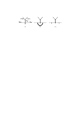
FIG. 2.: Feynman diagrams associated with the operator $O_{7}$. (a) shows the lowest order diagram, (b) and (c) show virtual- and bremsstrahlung corrections, respectively. The cross denotes the possible emission of the gluon.

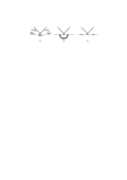
FIG. 3.: Feynman diagrams associated with the operators $O_{9}$ and $O_{10}$. (a) shows the lowest order diagrams, (b) and (c) show virtual- and bremsstrahlung corrections, respectively.

As in our previous works on $d\Gamma/d\hat{s}$, we use for the derivation of the double differential decay width a non-vanishing strange quark mass as a regulator of the collinear singularities and dimensional regularization ($d=4-2\epsilon$) for the infrared singularities. In the usual derivation of the decay width $d\Gamma/d\hat{s}$ one integrates out the lepton variables in the first step, after inserting a factor 1 in the form of eq. (14). It turns out that in the Dirac trace of the lepton tensor $L_{\mu\nu}$ the terms with an odd number of $\gamma_{5}$ matrices become zero after this integration. Furthermore, as the integrated lepton tensor is symmetric in $\mu$ and $\nu$, it follows that also in the hadron tensor (which is contracted with the lepton tensor over the indices $\mu$ and $\nu$) only traces with an even number of $\gamma_{5}$ matrices survive. Therefore, the $\gamma_{5}$ problems which usually appear in $d$-dimensions, can be avoided when calculating $d\Gamma/d\hat{s}$. These statements are no longer true if one aims to calculate the double differential decay width, which means that traces with an odd number of $\gamma_{5}$ matrices are unavoidable.

In our derivation of the virtual corrections to the double differential decays width, we calculated the loop corrections to the matrix elements as in our previous papers [42, 43], viz. using anticommuting $\gamma_{5}$ and letting propagate all $d$ polarizations of the virtual gluon in the loop. Using $(d-1)$-dimensional rotation invariance, the momenta of the external particles can be assumed to lie in four dimensions. Therefore, to proceed from the regulated matrix elements to the double differential decay width, we do the remaining Dirac algebra in $d=4$ dimensions. The subsequent phase space integrals are, however, treated in $d$ dimensions.

We now turn to the bremsstrahlung corrections. When calculating the squares of the matrix elements associated with $O_{7}$, $O_{9}$, $O_{10}$ (and interference terms) some care has to be taken in order to do the infrared regularization consistently. As in the virtual corrections all $d$ gluon polarizations were allowed to propagate, we have to emit all $d-2$ transverse polarizations in the bremsstrahlung process. As shown in refs. [53, 54], this can be implemented by doing the Dirac algebra in $d=4$ by summing the contributions from the emission of a gluon with the 2 possible transverse directions in four dimensions (characterized by normal 4-dimensional polarization vectors), and from the emission of the $(d-4)$ transverse polarizations showing in the $d-4$ extra dimensions. Each of the latter couples to the quarks (which remain in four dimensions) with a $\gamma_{5}$. The subsequent phase space integrations are again worked out in $d$-dimensions.

VI Phase space

A Fully differential phase space formula for lepton pair at rest

Starting from the well-known expression for the differential decay width for the process $b\rightarrow s\ell^{+}\ell^{-}$ and inserting a unit factor according to eq. (14), one obtains

$$d\Gamma^{\text{b-rest}}(b\rightarrow s\ell^{+}\ell^{-})=\frac{\overline{|M|^{2}}}{2\,m_{b}}\,D\Phi^{\text{b-rest}}\,,$$ (52)

where $\overline{|M|^{2}}$ is the squared matrix element, summed and averaged over spins and colors of the particles in the final- and initial state, respectively. Note that in our application $\overline{|M|^{2}}$ depends only on scalar products of four-vectors. $D\Phi^{\text{b-rest}}$ is the phase space factor which can be written as

$$D\Phi^{\text{b-rest}}=D\Phi^{\text{b-rest}}_{1}\,D\Phi^{\text{b-rest}}_{2}\,ds\,,$$ (53)

$$D\Phi^{\text{b rest}}_{1}=(2\pi)^{d}\,\frac{d^{d-1}q}{2q^{0}}\,\frac{d^{d-1}p_{s}}{(2\pi)^{d-1}2p_{s}^{0}}\,\delta^{d}(p_{b}-p_{s}-q)\,,$$ (54)

$$D\Phi^{\text{b-rest}}_{2}=\frac{d^{d-1}l_{1}}{(2\pi)^{d-1}2l_{1}^{0}}\,\frac{d^{d-1}l_{2}}{(2\pi)^{d-1}2l_{2}^{0}}\,\delta^{d}(q-l_{1}-l_{2})\,.$$ (55)

$p_{b}$, $p_{s}$, $l_{1}$, $l_{2}$ denote the four-momenta of the $b$-quark, the $s$-quark, the negatively and positively charged leptons, respectively, while $q=(l_{1}+l_{2})$, $q^{0}=\sqrt{\vec{q}^{2}+s}$ and $s=q^{2}$. Note that eqs. (52) and (53) generate the correct distributions of the decay products for a $b$-quark decay at rest or with fixed velocity.

Our main goal is to calculate the double differential decay width $\frac{d^{2}\Gamma(b\rightarrow X_{s}l^{+}l^{-})}{d\hat{s}dz}$, where $\hat{s}=s/m_{b}^{2}$ and $z=\cos\theta$ with $\theta$ being the angle between the momenta of the $b$-quark and the $\ell^{+}$, measured in the rest frame of the $(\ell^{+}\ell^{-})$-pair. For this purpose it is convenient to first derive a fully differential phase space formula in the rest frame of the lepton pair. In the following, unprimed momenta refer to the rest frame of the $b$-quark and primed ones to the corresponding momenta in the rest frame of the lepton pair. While in the rest frame of the $b$-quark the value of the vector $\vec{q}=\vec{l}_{1}+\vec{l}_{2}$ varies from event to event, it is $\vec{p^{\prime}_{b}}$ which varies from event to event in the rest frame of the lepton pair. The relation between $\vec{q}$ and $\vec{p^{\prime}}_{b}$ can be found from the equation

$$p^{\prime}_{b}=\Lambda_{q}\,p_{b}\,;\quad p_{b}=(m_{b},\vec{0})\,,$$ (56)

where $\Lambda_{q}$ is the Lorentz boost, which transforms the vector $\vec{q}$ to rest. We obtain

$$\vec{p^{\prime}_{b}}=-\frac{m_{b}}{\sqrt{s}}\vec{q}\quad(\mbox{and}\,\,\,p_{b}^{{}^{\prime}0}=\frac{m_{b}}{\sqrt{s}}\,q^{0})\,.$$ (57)

In the expression for the decay width this relation is most easily implemented by multiplying eq. (52) with a factor 1 in the form

$$1=\int\,d^{d-1}p^{\prime}_{b}\,\delta^{d-1}(\vec{p^{\prime}}_{b}+\frac{m_{b}}{\sqrt{s}}\,\vec{q})\,.$$ (58)

We anticipate that the integration over the variable $\vec{q}$ will finally perform the variable transformation $\vec{q}\leftrightarrow\vec{p^{\prime}}_{b}$. However, before doing this step we express all the unprimed momenta in the matrix element squared and in the delta functions with their primed counterparts, e.g. $l_{2}=\Lambda_{q}^{-1}l_{2}^{\prime}$, etc.. Note that due to Lorentz invariance of $\overline{|M|^{2}}$, this quantity is independent of $\Lambda_{q}^{-1}$, and therefore independent of $\vec{q}$. The same is also true for the measure factors of the final state particles and for the $d$-dimensional $\delta$-functions in eq. (53). The only remaining $\vec{q}$ dependence is contained in the term

$\displaystyle\frac{d^{d-1}q}{2\,q^{0}}\,\delta^{d-1}(\vec{p^{\prime}_{b}}+\frac{m_{b}}{\sqrt{s}}\,\vec{q})\,.$Integrating this eq. over $\vec{q}$, one obtains

$\displaystyle\int\frac{d^{d-1}q}{2\,q^{0}}\,\delta^{d-1}(\vec{p^{\prime}_{b}}+\frac{m_{b}}{\sqrt{s}}\,\vec{q})=\left(\frac{\sqrt{s}}{m_{b}}\right)^{d-2}\,\frac{1}{2\,p_{b}^{{}^{\prime}0}}\,.$To summarize: The expression for the fully differential decay width $d\Gamma(b\rightarrow s\ell^{+}\ell^{-})$ in the rest frame of the lepton pair can be written as

$$d\Gamma(b\rightarrow s\ell^{+}\ell^{-})=\frac{\overline{|M|^{2}}}{2\,m_{b}}\,D\Phi\,,$$ (59)

with

$$D\Phi=D\Phi_{1}\,D\Phi_{2}\,ds\,,$$ (60)

$$D\Phi_{1}=(2\pi)^{d}\,\left(\frac{\sqrt{s}}{m_{b}}\right)^{d-2}\,\frac{d^{d-1}p_{b}}{2p_{b}^{0}}\,\frac{d^{d-1}p_{s}}{(2\pi)^{d-1}2p_{s}^{0}}\,\delta^{d}(p_{b}-p_{s}-q)\,,$$ (61)

$$D\Phi_{2}=\frac{d^{d-1}l_{1}}{(2\pi)^{d-1}2l_{1}^{0}}\,\frac{d^{d-1}l_{2}}{(2\pi)^{d-1}2l_{2}^{0}}\,\delta^{d}(q-l_{1}-l_{2})\,.$$ (62)

As all momenta refer to the rest frame of the lepton pair, we omitted the primes in eqs. (59) and (60).

For the case of real gluon emission, $b\rightarrow sg\ell^{+}\ell^{-}$, the expression for the fully differential decay width in the rest frame of the $(\ell^{+}\ell^{-})$-pair can be derived in an analogous way. We obtain

$$d\Gamma(b\rightarrow sg\ell^{+}\ell^{-})=\frac{\overline{|M|^{2}}}{2\,m_{b}}\,D\Phi^{\text{brems}}\,,$$ (63)

$$D\Phi^{\text{brems}}=D\Phi^{\text{brems}}_{1}\,D\Phi_{2}\,ds\,,$$ (64)

$$D\Phi^{\text{brems}}_{1}=(2\pi)^{d}\,\left(\frac{\sqrt{s}}{m_{b}}\right)^{d-2}\,\frac{d^{d-1}p_{b}}{2p_{b}^{0}}\,\frac{d^{d-1}p_{s}}{(2\pi)^{d-1}2p_{s}^{0}}\,\frac{d^{d-1}r}{(2\pi)^{d-1}2r^{0}}\,\delta^{d}(p_{b}-r-p_{s}-q)\,.$$ (65)

$D\Phi_{2}$ is the same as in eq. (60) and $r$ is the four-momentum of the gluon.

B Phase space integrations

In this subsection we present the results for the phase space formulas for the double differential decay width where we integrate over the variables constrained by the $\delta$-functions and over the variables on which $\overline{|M|^{2}}$ does not depend.

To get the desired expression for the bremsstrahlung process, we start from eq. (63) and integrate over $\vec{l}_{1}$ and $\vec{p}_{s}$ by making use of the spacial parts of the two $d$-dimensional $\delta$-functions. Using then rotation invariance in ($d-1$) dimensions, we can assume that in $\overline{|M|^{2}}$ the “three-momenta” of the remaining particles have the form

$$\vec{p}_{b} = (|\vec{p}_{b}|,0,0;....)\,,$$ (66)

$$\vec{l}_{2} = (E_{2}\cos\theta,E_{2}\sin\theta,0;....)\,,$$ (67)

$$\vec{r} = (E_{r}\cos\theta_{1},E_{r}\sin\theta_{1}\cos\theta_{2},E_{r}\sin\theta_{1}\sin\theta_{2};....)\,,$$ (68)

where the dots symbolize the components of extra space dimensions, which are all zero. $E_{2}$ and $E_{r}$ are the energies of the massless positively charged lepton and the gluon, respectively. Making use of the remaining two one-dimensional $\delta$-functions, we can express $E_{2}$ and $\theta_{1}$ in terms of the other variables as

$$E_{2}=\frac{\sqrt{s}}{2}\quad;\quad\cos\theta_{1}=\frac{2E_{b}\sqrt{s}-2E_{r}\sqrt{s}+2E_{r}E_{b}-s-m_{b}^{2}+m_{s}^{2}}{2E_{r}|\vec{p}_{b}|}\,.$$ (69)

$E_{b}$ is the energy of the $b$-quark and $\sqrt{s}$ is the invariant mass of the lepton pair. After integration over the additional polar angles of $\vec{p}_{b}$, $\vec{l}_{2}$ and $\vec{r}$, on which $\overline{|M|^{2}}$ does not depend, we obtain (using $z=\cos\theta$, $z_{2}=\cos\theta_{2}$, $\hat{s}=s/m_{b}^{2}=q^{2}/m_{b}^{2}$, $d=4-2\epsilon$)

$$\frac{d^{2}\Gamma(b\rightarrow sg\ell^{+}\ell^{-})}{d\hat{s}\,dz} = \left(\frac{\mu^{2}\,\mbox{e}^{\gamma}}{4\pi}\right)^{3\epsilon}\,\frac{m_{b}^{1-2\epsilon}\,\hat{s}^{1-2\epsilon}}{(2\pi)^{3d-4}\,2^{7-4\epsilon}}\,\Omega_{d-1}\,\Omega_{d-2}\,\Omega_{d-3}\,\times$$ (71)

$$\int\,\overline{|M|^{2}}\,W^{-\epsilon}\,(1-z^{2})^{-\epsilon}\,(1-z_{2}^{2})^{-1/2-\epsilon}\,dz_{2}\,dE_{r}\,dE_{b}\,,$$

where $W$ reads

$\displaystyle W=4\,(E_{r}-E_{r}^{\rm{min}})\,(E_{r}^{\rm{max}}-E_{r})\,(m_{b}^{2}-2\sqrt{s}\,E_{b}+s)\,.$The three factors $\Omega$ stem from the integration over the polar angles on which $\overline{|M|^{2}}$ does not depend (explicitly, $\Omega_{d}=2\pi^{d/2}/\Gamma(d/2)$). The boundaries of the integration variables are

$$E_{r}^{\rm{min}}=\frac{m_{b}^{2}+s-2E_{b}\sqrt{s}-m_{s}^{2}}{2(E_{b}+|\vec{p}_{b}|-\sqrt{s})}\leq E_{r} \leq\frac{m_{b}^{2}+s-2E_{b}\sqrt{s}-m_{s}^{2}}{2(E_{b}-|\vec{p}_{b}|-\sqrt{s})}=E_{r}^{\rm{max}}\,,$$ (72)

$$m_{b}\leq E_{b} \leq\frac{m_{b}^{2}+s-m_{s}^{2}}{2\sqrt{s}}\,,$$ (73)

$$-1\leq z_{2} \leq 1\,.$$ (74)

To get the corresponding expression for the double differential decay width for the process $b\rightarrow s\ell^{+}\ell^{-}$, we start from eq. (59) and integrate over $\vec{l}_{1}$ and $\vec{p}_{s}$ by making use of the spacial parts of the two $d$-dimensional $\delta$-functions. Using rotation invariance, the three momenta of the remaining particles ($b$-quark and $\ell^{+}$) can be assumed to have the form as in eq. (66). The remaining two one-dimensional $\delta$-functions can be used to express the energy $E_{b}$ of the $b$-quark and the energy $E_{2}$ of $\ell^{+}$ in terms of $s$. Explicitly, we obtain

$\displaystyle E_{b}=\frac{m_{b}^{2}+s-m_{s}^{2}}{2\sqrt{s}}\quad;\quad E_{2}=\frac{\sqrt{s}}{2}\,.$After integration over the angles of $\vec{p}_{b}$ and $\vec{l}_{2}$, on which $\overline{|M|^{2}}$ does not depend, we obtain

$$\frac{d^{2}\Gamma(b\rightarrow s\ell^{+}\ell^{-})}{d\hat{s}\,dz} = \left(\frac{\mu^{2}\,\mbox{e}^{\gamma}}{4\pi}\right)^{2\epsilon}\,\frac{m_{b}^{-2\epsilon}\,\hat{s}^{1/2-2\epsilon}}{(2\pi)^{2d-3}\,2^{6-2\epsilon}}\,\Omega_{d-1}\,\Omega_{d-2}\,\overline{|M|^{2}}\,(1-z^{2})^{-\epsilon}\,|\vec{p}_{b}|^{d-3}\,.$$ (75)

VII Calculation of the sum of virtual- and bremsstrahlung corrections associated with $\boldsymbol{O_{7}}$, $\boldsymbol{O_{9}}$ and $\boldsymbol{O_{10}}$

In this section, we explain in some detail the tricks which allow to construct the functions $f_{99}$ and $f_{910}$ in eq. (20) in a simplified manner. The other functions $f_{77}$, $f_{79}$ and $f_{710}$ can be obtained in an analogous way. We use the notations

$\displaystyle\Gamma_{ij}(\hat{s},z)=\frac{d^{2}\Gamma_{ij}}{d\hat{s}\,dz}\quad\mbox{and}\quad\Gamma_{ij}(\hat{s})=\frac{d\Gamma_{ij}}{d\hat{s}}\quad(i\leq j)$for the contributions of the pair $(\widetilde{O}_{i},\widetilde{O}_{j})$ to the double differential decay width and to the invariant mass distribution, respectively. To make explicit the lowest order piece (⁰), the virtual- (^v) and bremsstrahlung (^b) corrections, we write

$$\Gamma_{ij}(\hat{s},z) = \Gamma_{ij}^{0}(\hat{s},z)+\Gamma_{ij}^{v}(\hat{s},z)+\Gamma_{ij}^{b}(\hat{s},z)\,,$$ (76)

$$\Gamma_{ij}(\hat{s}) = \Gamma_{ij}^{0}(\hat{s})+\Gamma_{ij}^{v}(\hat{s})+\Gamma_{ij}^{b}(\hat{s})\,.$$ (77)

As mentioned in section III, the virtual corrections to the matrix element were written in our earlier papers as multiples of tree-level matrix elements, explicitly

$$\langle s\ell^{+}\ell^{-}|\widetilde{O}_{7}|b\rangle_{\rm{virt}} = -\frac{\alpha_{s}}{4\pi}\,F_{7}^{(7)}\,\langle\widetilde{O}_{7}\rangle_{\rm{tree}}-\frac{\alpha_{s}}{4\pi}\,F_{7}^{(9)}\,\langle\widetilde{O}_{9}\rangle_{\rm{tree}}\,,$$ (78)

$$\langle s\ell^{+}\ell^{-}|\widetilde{O}_{9}|b\rangle_{\rm{virt}} = -\frac{\alpha_{s}}{4\pi}\,F_{9}^{(7)}\,\langle\widetilde{O}_{7}\rangle_{\rm{tree}}-\frac{\alpha_{s}}{4\pi}\,F_{9}^{(9)}\,\langle\widetilde{O}_{9}\rangle_{\rm{tree}}\,,$$ (79)

$$\langle s\ell^{+}\ell^{-}|\widetilde{O}_{10}|b\rangle_{\rm{virt}} = -\frac{\alpha_{s}}{4\pi}\,F_{9}^{(7)}\,\langle\widetilde{O}_{7,5}\rangle_{\rm{tree}}-\frac{\alpha_{s}}{4\pi}\,F_{9}^{(9)}\,\langle\widetilde{O}_{10}\rangle_{\rm{tree}}\,.$$ (80)

Note that $\langle\widetilde{O}_{7,5}\rangle_{\rm{tree}}$ is obtained from $\langle\widetilde{O}_{7}\rangle_{\rm{tree}}$ by replacing the lepton vector current by the corresponding axial vector current. As the explicit form of the (infrared singular) functions $F_{9}^{(9)}$ and $F_{7}^{(7)}$ is not needed in the following construction, we only list $F_{9}^{(7)}$ and $F_{7}^{(9)}$:

$$F_{9}^{(7)}(\hat{s})=\frac{2}{3}\ln(1-\hat{s})\,;\quad F_{7}^{(9)}(\hat{s})=\frac{16}{3\,\hat{s}}\ln(1-\hat{s})\,.$$ (81)

A Construction of $\boldsymbol{f_{99}(\hat{s},z)}$

The virtual corrections to the double- or single differential decay width are now readily obtained. For $\Gamma_{99}^{v}(\hat{s},z)$ and $\Gamma_{99}^{v}(\hat{s})$ we get

$$\Gamma_{99}^{v}(\hat{s},z) = -\frac{2\alpha_{s}}{4\pi}F_{9}^{(9)}(\hat{s})\,\Gamma^{0}_{99}(\hat{s},z)-\frac{\alpha_{s}}{4\pi}F_{9}^{(7)}(\hat{s})\,\Gamma^{0}_{79}(\hat{s},z)\,,$$ (82)

$$\Gamma_{99}^{v}(\hat{s}) = -\frac{2\alpha_{s}}{4\pi}F_{9}^{(9)}(\hat{s})\,\Gamma^{0}_{99}(\hat{s})-\frac{\alpha_{s}}{4\pi}F_{9}^{(7)}(\hat{s})\,\Gamma^{0}_{79}(\hat{s})\,.$$ (83)

We note that $\Gamma^{0}_{99}(\hat{s},z)$ and $\Gamma^{0}_{99}(\hat{s})$ are understood to be evaluated in $d$-dimensions as described in sections V and VI, because the function $F_{9}^{(9)}$ is infrared singular.

We now turn to the crucial point of our construction, which drastically simplifies the calculation of the bremsstrahlung corrections. We form the combination

$$\hat{\Gamma}^{v}_{99}(\hat{s},z)=\Gamma^{v}_{99}(\hat{s},z)-\frac{\Gamma^{0}_{99}(\hat{s},z)}{\Gamma^{0}_{99}(\hat{s})}\,\Gamma^{v}_{99}(\hat{s})\,,$$ (84)

in which the contributions proportional to the singular function $F_{9}^{(9)}$ drop out completely. $\hat{\Gamma}^{v}_{99}(\hat{s},z)$ is therefore finite. Explicitly, we get

$$\hat{\Gamma}^{v}_{99}(\hat{s},z)=\frac{\alpha_{s}}{4\pi}\,F_{9}^{(7)}(\hat{s})\,\frac{m_{b}^{5}\,\alpha_{\text{em}}^{2}\,G_{F}^{2}\,|V_{tb}V_{ts}^{*}|^{2}\,\widetilde{C}_{9}^{2}\,(1-\hat{s})^{3}\,(1-3z^{2})}{256\pi^{5}\,(1+2\hat{s})}.$$ (85)

We now form the analogous combination for the bremsstrahlung corrections, viz.

$$\hat{\Gamma}^{b}_{99}(\hat{s},z)=\Gamma^{b}_{99}(\hat{s},z)-\frac{\Gamma^{0}_{99}(\hat{s},z)}{\Gamma^{0}_{99}(\hat{s})}\,\Gamma^{b}_{99}(\hat{s})\,.$$ (86)

It follows from the Kinoshita-Lee-Neuenberg (KLN) theorem that $\hat{\Gamma}^{b}_{99}(\hat{s},z)$ must also be finite. Using eqs. (84) and (86), one can write the sum of the virtual- and bremsstrahlung corrections to the double differential decay width in the form

$$\Gamma^{v}_{99}(\hat{s},z)+\Gamma^{b}_{99}(\hat{s},z)=\hat{\Gamma}^{v}_{99}(\hat{s},z)+\hat{\Gamma}^{b}_{99}(\hat{s},z)+\frac{\Gamma^{0}_{99}(\hat{s},z)}{\Gamma^{0}_{99}(\hat{s})}\,\left(\Gamma^{v}_{99}(\hat{s})+\Gamma^{b}_{99}(\hat{s})\right)\,.$$ (87)

$\hat{\Gamma}^{v}_{99}(\hat{s},z)$ on the r.h.s of eq. (87) is given in eq. (85). $\left(\Gamma^{v}_{99}(\hat{s})+\Gamma^{b}_{99}(\hat{s})\right)$ is also known, viz.

$$\Gamma^{v}_{99}(\hat{s})+\Gamma^{b}_{99}(\hat{s})=\Gamma^{0}_{99}(\hat{s})\left(1+\frac{2\,\alpha_{s}}{\pi}\,\omega_{99}(\hat{s})\right)\,,$$ (88)

where $\omega_{99}(\hat{s})$ is given in refs. [42, 43] (see also eq. (A4)). $\Gamma^{0}_{99}(\hat{s},z)$ which in eq. (87) is only needed in $d=4$ dimensions, reads

$$\Gamma^{0}_{99}(\hat{s},z)=\frac{m_{b}^{5}\,\alpha_{\text{em}}^{2}\,G_{F}^{2}\,|V_{tb}V_{ts}^{*}|^{2}\,\widetilde{C}_{9}^{2}}{1024\pi^{5}}\,(1-\hat{s})^{2}\left[(1-z^{2})+\hat{s}(1+z^{2})\right]\,.$$ (89)

This implies that the sum of virtual- and bremsstrahlung corrections to the double differential decay width, and hence the function $f_{99}(\hat{s},z)$ in eq. (7), is easily obtained once the finite combination $\hat{\Gamma}^{b}_{99}(\hat{s},z)$ in eq. (86) is known.

B Construction of $\boldsymbol{f_{910}(\hat{s})}$

As $\Gamma_{910}^{0}(\hat{s})$ turns out to be zero, one cannot take the combination analogous to eq. (84). Instead, we use the combination

$$\hat{\Gamma}^{v}_{910}(\hat{s},z)=\Gamma^{v}_{910}(\hat{s},z)-\frac{\Gamma^{0}_{910}(\hat{s},z)}{\Gamma^{0}_{99}(\hat{s})}\,\Gamma^{v}_{99}(\hat{s})\,.$$ (90)

Again, the part proportional to the singular function $F_{9}^{(9)}$ drops out and $\hat{\Gamma}^{v}_{910}(\hat{s},z)$ is finite. Explicitly, we find

$$\hat{\Gamma}^{v}_{910}(\hat{s},z)=\frac{2\alpha_{s}}{4\pi}\,F_{9}^{(7)}(\hat{s})\,\frac{m_{b}^{5}\,\alpha_{\text{em}}^{2}\,G_{F}^{2}\,|V_{tb}V_{ts}^{*}|^{2}\,\widetilde{C}_{9}\,\widetilde{C}_{10}\,(1-\hat{s})^{3}\,z}{128\pi^{5}\,(1+2\hat{s})}.$$ (91)

The analogous combination for the bremsstrahlung corrections, viz.

$$\hat{\Gamma}^{b}_{910}(\hat{s},z)=\Gamma^{b}_{910}(\hat{s},z)-\frac{\Gamma^{0}_{910}(\hat{s},z)}{\Gamma^{0}_{99}(\hat{s})}\,\Gamma^{b}_{99}(\hat{s})\,$$ (92)

is also finite. From eqs. (90) and (92) one gets

$$\Gamma^{v}_{910}(\hat{s},z)+\Gamma^{b}_{910}(\hat{s},z)=\hat{\Gamma}^{v}_{910}(\hat{s},z)+\hat{\Gamma}^{b}_{910}(\hat{s},z)+\frac{\Gamma^{0}_{910}(\hat{s},z)}{\Gamma^{0}_{99}(\hat{s})}\,\left(\Gamma^{v}_{99}(\hat{s})+\Gamma^{b}_{99}(\hat{s})\right)\,.$$ (93)

$\hat{\Gamma}^{v}_{910}(\hat{s},z)$ and $\left(\Gamma^{v}_{99}(\hat{s})+\Gamma^{b}_{99}(\hat{s})\right)$ are given in eqs. (91) and (88), respectively. $\Gamma^{0}_{910}(\hat{s},z)$ which is only needed in $d=4$ dimensions in eq. (93), reads

$$\Gamma^{0}_{910}(\hat{s},z)=-\frac{m_{b}^{5}\,\alpha_{\text{em}}^{2}\,G_{F}^{2}\,|V_{tb}V_{ts}^{*}|^{2}\,\widetilde{C}_{9}\,\widetilde{C}_{10}}{256\pi^{5}}\,(1-\hat{s})^{2}\,\hat{s}\,z\,.$$ (94)

This implies that the function $f_{910}(\hat{s})$ is easily obtained, once the finite combination $\hat{\Gamma}^{b}_{910}(\hat{s},z)$ defined in eq. (92) is known.

To obtain the functions $f_{77}(\hat{s},z)$, $f_{79}(\hat{s},z)$ and $f_{710}(\hat{s})$, one can proceed in a similar way. Forming suitable combinations, the hardest part of the calculation of these functions boils down to the evaluation of a finite combination of bremsstrahlung terms.

A remark concerning to the evaluation of the finite bremsstrahlung combinations is in order: We carefully investigated all five combinations (needed to construct the five $f$-functions) in $d=4-2\epsilon$ dimensions, as in principle terms of order $\epsilon^{1}$ from the phase space factors could multiply divergent integrals and in this way generate finite terms. We found, however, that this case does not occur in our actual calculations: Expanding all combinations up to order $\epsilon$ (or even $\epsilon^{2}$) before doing the phase space integrations over the variables $E_{r}$ and $E_{b}$ (see section VI), we found that all the occurring integrals are finite. This means, that it is correct to evaluate the finite combinations in $d=4$ dimensions.

VIII Phenomenological analysis

FIG. 4.: Left frame: Unnormalized forward-backward asymmetry $A_{\text{FB}}(\hat{s})$. The three solid lines show the NNLL prediction for $\mu=2.5,5.0,10.0$ GeV, respectively. The corresponding curves in NLL approximation are shown by dashed lines. Right frame: Normalized forward-backward asymmetry $\overline{A}_{\text{FB}}(\hat{s})$. The lines have the same meaning as in the left frame. $m_{c}/m_{b}=0.29$.

In this section, we mainly investigate the impact of the NNLL QCD corrections on the forward-backward asymmetries defined in eqs. (21) and (22) in the standard model. We restrict ourselves to the range of $\hat{s}=s/m_{b}^{2}$ below 0.25, i.e., to the region below the $J/\psi$ threshold. As our main emphasis is to investigate the improvements in the perturbative part, in particular the reduction of the renormalization scale dependence, we do not include non-perturbative corrections, although in this $\hat{s}$-region they are known to a large extent [28, 31, 32, 33, 34, 35]. In our analysis, we use the following fixed values for the input parameters: $m_{b}^{\rm{pole}}=4.8$ GeV, $\alpha_{\text{em}}=1/133$, $\mbox{BR}_{\text{sl}}=0.104$, $m_{t}^{\rm{pole}}=174$ GeV, $\alpha_{s}(m_{Z})=0.119$ and $|V_{tb}\,V_{ts}|/|V_{cb}|=0.976$. The values of $m_{c}/m_{b}$ and of the renormalization scale $\mu$ are specified in the captions of the individual figures.

In figs. 4 we illustrate the reduction of the renormalization scale dependence of the forward-backward asymmetries when taking into account NNLL QCD corrections. As usual, the renormalization scale is varied between 2.5 GeV and 10.0 GeV. For definiteness, we should mention that in the unnormalized forward-backward asymmetry $A_{\text{FB}}(\hat{s})$, we evaluated the denominator $\Gamma(B\rightarrow X_{c}e\bar{\nu}_{e})$ in eq. (22) always at $\mu=5$ GeV. The results are remarkable: While the NLL asymmetries (shown by dashed lines for $\mu$=2.5, 5.0 and 10 GeV) suffered from a relatively large renormalization scale dependence, the theoretical uncertainty related to the choice of the renormalization scale is significantly reduced at the NNLL level. For example, at $\hat{s}=0$ we find

$$A_{\text{FB}}^{\text{NLL}}(0)=-(2.51\pm 0.28)\times 10^{-6}\,;\quad A_{\text{FB}}^{\text{NNLL}}(0)=-(2.30\pm 0.10)\times 10^{-6}\,.$$ (95)

This corresponds to a reduction of the $\mu$-dependence from $\pm 11\%$ to $\pm 4.5\%$, which is similar to the situation found for the differential branching ratio in ref. [43]. When looking at the position $\hat{s}_{0}$, where the forward-backward asymmetries are zero, the reduction of the $\mu$-dependence at NNLL is even stronger. We find (when only taking into account the error due to the $\mu$-dependence)

$$\hat{s}_{0}^{\rm{NLL}}=0.144\pm 0.020\,;\quad\hat{s}_{0}^{\rm{NNLL}}=0.162\pm 0.002\,.$$ (96)

FIG. 5.: Left frame: Unnormalized forward-backward asymmetry $A_{\text{FB}}(\hat{s})$. The three solid lines show the NNLL prediction for $\mu=2.5,5.0,10.0$ GeV, respectively. The dashed lines show the corresponding results when switching off the functions $f_{710}(\hat{s})$ and $f_{910}(\hat{s})$. Right frame: Normalized forward-backward asymmetry $\overline{A}_{\text{FB}}(\hat{s})$. The three solid lines show the NNLL prediction for $\mu=2.5,5.0,10.0$ GeV, respectively. The dashed lines show the corresponding results when switching off the functions $f_{710}(\hat{s})$, $f_{910}(\hat{s})$, $\omega_{77}(\hat{s})$, $\omega_{99}(\hat{s})$, and $\omega_{79}(\hat{s})$. $m_{c}/m_{b}=0.29$.

The parts of the NNLL corrections to the forward-backward asymmetries which are contained in the effective Wilson coefficients $\widetilde{C}_{7}^{\text{eff}}$, $\widetilde{C}_{9}^{\text{eff}}$ and $\widetilde{C}_{10}^{\text{eff}}$ (see eqs. (12)-(13)), i.e., the virtual corrections to the matrix elements of the operators $O_{1}$, $O_{2}$ and $O_{8}$ and the NNLL contributions to the Wilson coefficients, are known for quite some time. In figs. 5 we illustrate the importance of the new contributions related to virtual- and bremsstrahlung corrections to $O_{7}$, $O_{9}$ and $O_{10}$, which are encoded through the functions $f_{710}(\hat{s})$ and $f_{910}(\hat{s})$. The solid lines show the full NNLL results, while the dashed ones are obtained by switching off the functions $f_{710}(\hat{s})$ and $f_{910}(\hat{s})$ (in the case of the normalized forward-backward asymmetry also the functions $\omega_{99}(\hat{s})$, $\omega_{77}(\hat{s})$ and $\omega_{79}(\hat{s})$ are switched off). We find that the new contributions are crucial, in particular for the reduction of the renormalization scale dependence.

FIG. 6.: Left frame: Unnormalized forward-backward asymmetry $A_{\text{FB}}(\hat{s})$. The three lines show the NNLL prediction for $m_{c}^{\text{pole}}/m_{b}^{\text{pole}}=0.25,0.29,0.33$, respectively. The renormalization scale is $\mu=5$ GeV. Right frame: The same for the normalized forward-backward asymmetry $\overline{A}_{\text{FB}}(\hat{s})$.

As found in refs. [43, 44], the error on the decay width $d\Gamma(b\rightarrow X_{s}\ell^{+}\ell^{-})/d\hat{s}$ due to uncertainties in the input parameters is by far dominated by the uncertainty of the charm quark mass $m_{c}$. In principle, there are two sources for this uncertainty. First, it is unclear whether $m_{c}$ in the virtual- and bremsstrahlung corrections should be interpreted as the pole mass or the $\overline{\mbox{MS}}$ mass (at an appropriate scale). Second, the question arises what the numerical value of $m_{c}$ is, once a choice concerning the definition of $m_{c}$ has been made. These issues were investigated in detail in ref. [44] and led to the conclusion that the error due to uncertainties in the parameter $m_{c}/m_{b}$ is conservatively estimated when using for this quantity $m_{c}^{\rm{pole}}/m_{b}^{\rm{pole}}=0.29\pm 0.04$. For a discussion of the corresponding questions for the process $B\rightarrow X_{s}\gamma$, we refer to [13]. Motivated by these studies, we illustrate in figs. 6 the dependence of the forward-backward asymmetries on $m_{c}^{\rm{pole}}/m_{b}^{\rm{pole}}$. The three lines show the asymmetries for the values $m_{c}^{\rm{pole}}/m_{b}^{\rm{pole}}$=0.25, 0.29 and 0.33. We find that for most values of $\hat{s}$ the charm quark mass dependence of the normalized forward-backward asymmetry $\overline{A}_{\text{FB}}(\hat{s})$ is smaller than the one of the unnormalized counterpart $A_{\text{FB}}(\hat{s})$. This is related to the fact that a relatively large charm quark mass dependence enters the observable $A_{\text{FB}}(\hat{s})$ through the semileptonic decay width present in the defining eq. (22); this is not the case for the normalized version (see eq. (21)). For $\hat{s}_{0}$, the position where the forward-backward asymmetries vanish, we find (when taking into account only the error due to $m_{c}/m_{b}$)

$$\hat{s}_{0}^{\rm{NNLL}}=0.162\pm 0.005\,.$$ (97)

FIG. 7.: Left frame: NNLL branching ratio differential in $z=\cos\theta$ for four bins in $\hat{s}$. Bin 1: $0.05\leq\hat{s}\leq 0.10$ (solid); bin 2: $0.10\leq\hat{s}\leq 0.15$ (dotted); bin 3: $0.15\leq\hat{s}\leq 0.20$ (short-dashed); bin 4: $0.20\leq\hat{s}\leq 0.25$ (long-dashed). $m_{c}^{\text{pole}}/m_{b}^{\text{pole}}=0.29$ and $\mu=5$ GeV.
Right frame: NNLL branching ratio differential in $z=\cos\theta$. $\hat{s}$ is integrated in the interval $0.05\leq\hat{s}\leq 0.25$. The curves correspond to $\mu=2.5$ GeV (lowest), $\mu=5.0$ GeV (middle) and $\mu=10.0$ GeV (uppermost). $m_{c}^{\text{pole}}/m_{b}^{\text{pole}}=0.29$.

We expect that in the future also the angular distribution in $\theta$ will become measurable. In the left frame in fig. 7 we show the branching ratio differential in the variable $z=\cos\theta$ for four bins in $\hat{s}$, using $\mu=5$ GeV for the renormalization scale and putting $m_{c}^{\rm{pole}}/m_{b}^{\rm{pole}}=0.29$. In the right frame we show this branching ratio after integrating $\hat{s}$ over the interval $0.05\leq\hat{s}\leq 0.25$ for three values of the renormalization scale and putting $m_{c}^{\rm{pole}}/m_{b}^{\rm{pole}}=0.29$.

IX Summary

In this paper we presented NNLL results for the double differential decay width $d\Gamma(b\rightarrow X_{s}\ell^{+}\ell^{-})/(d\hat{s}\,dz)$. The variable $z$ denotes $\cos(\theta)$, where $\theta$ is the angle between the momenta of the $b$-quark and the $\ell^{+}$, measured in the rest-frame of the lepton pair. To obtain these results, genuinely new calculations were necessary for the combined virtual- and gluon bremsstrahlung corrections associated with the operators $O_{7}$, $O_{9}$ and $O_{10}$. These corrections are encoded in the functions $f_{99}(\hat{s},z)$, $f_{77}(\hat{s},z)$, $f_{79}(\hat{s},z)$, $f_{910}(\hat{s})$ and $f_{710}(\hat{s})$ in the general expression (20) for the double differential decay width. To obtain a NNLL prediction for this quantity, we combined these new ingredients with existing results on the NNLL Wilson coefficients and on the virtual corrections to the matrix elements of the operators $O_{1}$, $O_{2}$ and $O_{8}$. As the virtual QCD corrections to the matrix elements of $O_{1}$ and $O_{2}$ are only known for values of $\hat{s}\leq 0.25$, this implies that NNLL corrections to the double differential decay width are available only for values of $\sqrt{s}$ below the $J/\psi$ resonance. In this paper, we neglected certain bremsstrahlung contributions, which in principle contribute at NNLL precision. This omission is well motivated by the fact that the corresponding corrections have a very small impact on $d\Gamma(b\rightarrow X_{s}\ell^{+}\ell^{-})/d\hat{s}$.

From our results on the double differential decay width we derived NNLL results for the lepton forward-backward asymmetries, as these quantities are known to be very sensitive to new physics. We found that the NNLL corrections drastically reduce the renormalization scale ($\mu$) dependence of the forward-backward asymmetries. In particular, $\hat{s}_{0}$, the position at which the forward-backward asymmetries vanish, is essentially free of uncertainties due to the renormalization scale at NNLL precision. At NNLL precision, we found $\hat{s}_{0}^{\rm{NNLL}}=0.162\pm 0.005$, where the error is dominated the uncertainty in $m_{c}/m_{b}$. This is to be compared with the NLL result, $\hat{s}_{0}^{\rm{NLL}}=0.144\pm 0.020$, where the error is dominated by uncertainties due to the choice of $\mu$.

When we were working out the double differential decay width, a paper on the NNLL predictions for the forward-backward asymmetries was submitted to the hep-archive [49]. As these authors used a different regularization scheme for infrared- and collinear singularities and another procedure for the evaluation of the phase space integrals, the two papers provide independent calculations of the forward-backward asymmetries. Our results are in full agreement with those presented in their final version [49].

Acknowlegments: We thank Haik Asatrian and Manuel Walker for useful discussions.

A $\boldsymbol{\omega_{77}(\hat{s})$,$\omega_{99}(\hat{s})$and$\omega_{79}(\hat{s})}$

In this appendix we repeat the explicit expressions for the functions $\omega_{77}(\hat{s})$, $\omega_{99}(\hat{s})$ and $\omega_{79}(\hat{s})$ which contain the virtual- and bremsstrahlung corrections to the matrix elements associated with the operators $\widetilde{O}_{7}$, $\widetilde{O}_{9}$ and $\widetilde{O}_{10}$. For their derivation, we refer to [42, 43]. The functions read ($\text{Li}_{2}(x)=-\int_{0}^{x}\,dt/t\,\ln(1-t)$)

$$\omega_{77}(\hat{s}) = -\frac{8}{3}\,\ln\left(\frac{\mu}{m_{b}}\right)-\frac{4}{3}\,\text{Li}_{2}(\hat{s})-\frac{2}{9}\,{\pi}^{2}-\frac{2}{3}\,\ln(\hat{s})\ln(1-\hat{s})$$ (A2)

$$-\frac{1}{3}\,\frac{8+\hat{s}}{2+\hat{s}}\ln(1-\hat{s})-\frac{2}{3}\,\frac{\hat{s}\left(2-2\,\hat{s}-\hat{s}^{2}\right)}{\left(1-\hat{s}\right)^{2}\left(2+\hat{s}\right)}\ln(\hat{s})-\frac{1}{18}\,\frac{16-11\,\hat{s}-17\,\hat{s}^{2}}{\left(2+\hat{s}\right)\left(1-\hat{s}\right)}\,,$$

$$\omega_{99}(\hat{s}) = -\frac{4}{3}\,\text{Li}_{2}(\hat{s})-\frac{2}{3}\ln(1-\hat{s})\ln(\hat{s})-\frac{2}{9}\pi^{2}-\frac{5+4\,\hat{s}}{3(1+2\,\hat{s})}\ln(1-\hat{s})$$ (A4)

$$-\frac{2\,\hat{s}\,(1+\hat{s})(1-2\,\hat{s})}{3\,(1-\hat{s})^{2}(1+2\,\hat{s})}\ln(\hat{s})+\frac{5+9\,\hat{s}-6\,\hat{s}^{2}}{6\,(1-\hat{s})(1+2\,\hat{s})}\,,$$

$$\omega_{79}(\hat{s}) = -\frac{4}{3}\,\ln\left(\frac{\mu}{m_{b}}\right)-\frac{4}{3}\,\text{Li}_{2}(\hat{s})-\frac{2}{9}\,{\pi}^{2}-\frac{2}{3}\,\ln(\hat{s})\ln(1-\hat{s})$$ (A6)

$$-\frac{1}{9}\,\frac{2+7\,\hat{s}}{\hat{s}}\ln(1-\hat{s})-\frac{2}{9}\,\frac{\hat{s}\left(3-2\,\hat{s}\right)}{\left(1-\hat{s}\right)^{2}}\ln(\hat{s})+\frac{1}{18}\,\frac{5-9\,\hat{s}}{1-\hat{s}}\,.$$

B Auxiliary quantities $\boldsymbol{A_{i}}$, $\boldsymbol{T_{9}}$, $\boldsymbol{U_{9}}$ and $\boldsymbol{W_{9}}$

The auxiliary quantities $A_{i}$, $T_{9}$, $U_{9}$ and $W_{9}$ appearing in the effective Wilson coefficients in eqs. (10)–(13) are the following linear combinations of the Wilson coefficients $C_{i}(\mu)$ [41, 23]:

$$A_{7}= \,\frac{4\,\pi}{\alpha_{s}(\mu)}\,C_{7}(\mu)-\frac{1}{3}\,C_{3}(\mu)-\frac{4}{9}\,C_{4}(\mu)-\frac{20}{3}\,C_{5}(\mu)-\frac{80}{9}\,C_{6}(\mu)\,,$$ (B1)

$$A_{8}= \,\frac{4\,\pi}{\alpha_{s}(\mu)}\,C_{8}(\mu)+C_{3}(\mu)-\frac{1}{6}\,C_{4}(\mu)+20\,C_{5}(\mu)-\frac{10}{3}\,C_{6}(\mu)\,,$$ (B2)

$$A_{9}= \,\frac{4\pi}{\alpha_{s}(\mu)}\,C_{9}(\mu)+\sum_{i=1}^{6}\,C_{i}(\mu)\,\gamma_{i9}^{(0)}\,\ln\!\left(\frac{m_{b}}{\mu}\right)+\frac{4}{3}\,C_{3}(\mu)+\frac{64}{9}\,C_{5}(\mu)+\frac{64}{27}\,C_{6}(\mu)\,,$$ (B3)

$$A_{10}= \,\frac{4\pi}{\alpha_{s}(\mu)}\,C_{10}(\mu)\,,$$ (B4)

$$T_{9}= \,\frac{4}{3}\,C_{1}(\mu)+C_{2}(\mu)+6\,C_{3}(\mu)+60\,C_{5}(\mu)\,,$$ (B5)

$$U_{9}= -\frac{7}{2}\,C_{3}(\mu)-\frac{2}{3}\,C_{4}(\mu)-38\,C_{5}(\mu)-\frac{32}{3}\,C_{6}(\mu)\,,$$ (B6)

$$W_{9}= -\frac{1}{2}\,C_{3}(\mu)-\frac{2}{3}\,C_{4}(\mu)-8\,C_{5}(\mu)-\frac{32}{3}\,C_{6}(\mu)\,.$$ (B7)

The entries $\gamma_{i9}^{(0)}$ of the anomalous dimension matrix read for $i=1,...,6$: $(-32/27,-8/9,-16/9,32/27,-112/9,512/27)$. In the contributions which explicitly involve virtual or bremsstrahlung correction only the leading order coefficients $A_{i}^{(0)}$, $T_{9}^{(0)}$, $U_{9}^{(0)}$ and $W_{9}^{(0)}$ enter. They are given by

$$A_{7}^{(0)}= \,\,C_{7}^{(1)}-\frac{1}{3}\,C_{3}^{(0)}-\frac{4}{9}\,C_{4}^{(0)}-\frac{20}{3}\,C_{5}^{(0)}-\frac{80}{9}\,C_{6}^{(0)}\,,$$ (B8)

$$A_{8}^{(0)}= \,\,C_{8}^{(1)}+C_{3}^{(0)}-\frac{1}{6}\,C_{4}^{(0)}+20\,C_{5}^{(0)}-\frac{10}{3}\,C_{6}^{(0)}\,,$$ (B9)

$$A_{9}^{(0)}= \,\frac{4\,\pi}{\alpha_{s}}\left(C_{9}^{(0)}+\frac{\alpha_{s}}{4\,\pi}\,C_{9}^{(1)}\right)+\sum_{i=1}^{6}\,C_{i}^{(0)}\,\gamma_{i9}^{(0)}\,\ln\!\left(\frac{m_{b}}{\mu}\right)+\frac{4}{3}\,C_{3}^{(0)}+\frac{64}{9}\,C_{5}^{(0)}+\frac{64}{27}\,C_{6}^{(0)}\,,$$ (B10)

$$A_{10}^{(0)}= \,C_{10}^{(1)}\,,\vspace*{0.3cm}$$ (B11)

$$\vspace*{0.3cm}T_{9}^{(0)}= \,\frac{4}{3}\,C_{1}^{(0)}+C_{2}^{(0)}+6\,C_{3}^{(0)}+60\,C_{5}^{(0)}\,,$$ (B12)

$$U_{9}^{(0)}= -\frac{7}{2}\,C_{3}^{(0)}-\frac{2}{3}\,C_{4}^{(0)}-38\,C_{5}^{(0)}-\frac{32}{3}\,C_{6}^{(0)}\,,$$ (B13)

$$W_{9}^{(0)}= -\frac{1}{2}\,C_{3}^{(0)}-\frac{2}{3}\,C_{4}^{(0)}-8\,C_{5}^{(0)}-\frac{32}{3}\,C_{6}^{(0)}\,.$$ (B14)

We list the leading and next-to-leading order contributions to the quantities $A_{i}$, $T_{9}$, $U_{9}$ and $W_{9}$ in Tab. I.

$\mu$	$2.5$ GeV	$5$ GeV	$10$ GeV
$\alpha_{s}$	$0.267$	$0.215$	$0.180$
$C_{1}^{(0)}$	$-0.697$	$-0.487$	$-0.326$
$C_{2}^{(0)}$	$1.046$	$1.024$	$1.011$
$\raisebox{1.42262pt}{\big{(}}A_{7}^{(0)},~{}A_{7}^{(1)}\raisebox{1.42262pt}{\big{)}}$	$(-0.360,~{}0.031)$	$(-0.321,~{}0.019)$	$(-0.287,~{}0.008)$
$A_{8}^{(0)}$	$-0.164$	$-0.148$	$-0.134$
$\raisebox{1.42262pt}{\big{(}}A_{9}^{(0)},~{}A_{9}^{(1)}\raisebox{1.42262pt}{\big{)}}$	$(4.241,~{}-0.170)$	$(4.129,~{}0.013)$	$(4.131,~{}0.155)$
$\raisebox{1.42262pt}{\big{(}}T_{9}^{(0)},~{}T_{9}^{(1)}\raisebox{1.42262pt}{\big{)}}$	$(0.115,~{}0.278)$	$(0.374,~{}0.251)$	$(0.576,~{}0.231)$
$\raisebox{1.42262pt}{\big{(}}U_{9}^{(0)},~{}U_{9}^{(1)}\raisebox{1.42262pt}{\big{)}}$	$(0.045,~{}0.023)$	$(0.032,~{}0.016)$	$(0.022,~{}0.011)$
$\raisebox{1.42262pt}{\big{(}}W_{9}^{(0)},~{}W_{9}^{(1)}\raisebox{1.42262pt}{\big{)}}$	$(0.044,~{}0.016)$	$(0.032,~{}0.012)$	$(0.022,~{}0.009)$
$\raisebox{1.42262pt}{\big{(}}A_{10}^{(0)},~{}A_{10}^{(1)}\raisebox{1.42262pt}{\big{)}}$	$(-4.372,~{}0.135)$	$(-4.372,~{}0.135)$	$(-4.372,~{}0.135)$

TABLE I.: Coefficients appearing in eqs. (10)–(13) for $\mu=2.5$ GeV, $\mu=5$ GeV and $\mu=10$ GeV. For $\alpha_{s}(\mu)$ (in the $\overline{\mbox{MS}}$ scheme) we used the two-loop expression with five flavors and $\alpha_{s}(m_{Z})=0.119$. The entries correspond to the pole top quark mass $m_{t}=174$ GeV. The superscript (0) refers to lowest order quantities while the superscript (1) denotes the correction terms of order $\alpha_{s}$, i.e. $X=X^{(0)}+X^{(1)}$ with $X=C,A,T,U,W$.

Finally, we give the function $h(z,\hat{s})$ which appears in the effective Wilson coefficients in eqs. (10)–(13):

$$h(z,\hat{s}) = -\frac{4}{9}\ln(z)+\frac{8}{27}+\frac{16}{9}\frac{z}{\hat{s}}$$ (B16)

$$-\frac{2}{9}\left(2+\frac{4\,z}{\hat{s}}\right)\sqrt{\left|\frac{4\,z-\hat{s}}{\hat{s}}\right|}\cdot\begin{cases}2\arctan\sqrt{\frac{\hat{s}}{4\,z-\hat{s}}}\,\,,&\hat{s}<4\,z\\ \\ \ln\left(\frac{\sqrt{\hat{s}}+\sqrt{\hat{s}-4\,z}}{\sqrt{\hat{s}}-\sqrt{\hat{s}-4\,z}}\right)-i\,\pi,&\hat{s}>4\,z\end{cases}\,\,.$$

REFERENCES

• [1] R. Ammar et al. [CLEO Collaboration], Phys. Rev. Lett. 71, 674 (1993).
• [2] M. S. Alam et al. [CLEO Collaboration], Phys. Rev. Lett. 74, 2885 (1995).
• [3] R. Barate et al. [ALEPH Collaboration], Phys. Lett. B 429, 169 (1998).
• [4] K. Abe et al. [BELLE Collaboration], Phys. Lett. B 511, 151 (2001) [hep-ex/0103042].
• [5] B. Aubert et al. [BABAR Collaboration], hep-ex/0207074, hep-ex/0207076.
• [6] S. Chen et al. [CLEO Collaboration], Phys. Rev. Lett. 87, 251807 (2001) [hep-ex/0108032].
• [7] A. Ali and C. Greub, Zeit. f. Phys. C 49, 431 (1991); Phys. Lett. B 259, 182 (1991); Phys. Lett. B 361, 146 (1995).
A.L. Kagan and M. Neubert, Eur. Phys. J. C 7, 5 (1999).
• [8] K. Adel and Y. P. Yao, Phys. Rev. D 49, 4945 (1994);
C. Greub and T. Hurth Phys. Rev. D 56, 2934 (1997);
A. J. Buras, A. Kwiatkowski and N. Pott, Nucl. Phys. B 517, 353 (1998).
• [9] M. Ciuchini, G. Degrassi, P. Gambino and G. F. Giudice, Nucl. Phys. B 527, 21 (1998).
• [10] K. Chetyrkin, M. Misiak and M. Münz, Phys. Lett. B 400, 206 (1997); Nucl. Phys. B 518, 473 (1998); Nucl. Phys. B 520, 279 (1998).
• [11] C. Greub, T. Hurth and D. Wyler, Phys. Rev. D 54, 3350 (1996).
• [12] A. J. Buras, A. Czarnecki, M. Misiak, J. Urban, Nucl. Phys. B 611, 488 (2001) [hep-ph/0105160].
• [13] P. Gambino and M. Misiak, Nucl. Phys. B 611, 338 (2001) [hep-ph/0104034].
• [14] F. Borzumati and C. Greub, Phys. Rev. D 58, 074004 (1998); Phys. Rev. D 59, 057501 (1999).
• [15] H.H. Asatryan, H.M. Asatrian, G.K. Yeghiyan and G.K. Savvidy, Int. J. of Mod. Phys. A 16 3805 (2001).
• [16] G.M. Asatryan and A.N. Ioannisyan, Sov. J. Nucl. Phys. 51, 858 (1990); Mod. Phys. Lett. A 5, 1089 (1990).
• [17] S. Bertolini, F. Borzumati, A. Masiero and G. Ridolfi, Nucl. Phys. B 353, 591 (1991).
• [18] M. Ciuchini, G. Degrassi, P. Gambino and G.F. Giudice, Nucl. Phys. B 534, 3 (1998).
• [19] C. Bobeth, M. Misiak and J. Urban, Nucl. Phys. B 567, 153 (2000).
• [20] F. Borzumati, C. Greub, T. Hurth and D. Wyler, Phys. Rev. D 62, 075005 (2000).
• [21] H. H. Asatrian and H. M. Asatrian, Phys. Lett. B 460 (1999) 148.
• [22] T. Besmer, C. Greub and T. Hurth, Nucl. Phys. B 609, 359 (2001).
• [23] A. Ali, E. Lunghi, C. Greub, G. Hiller, Phys. Rev. D 66, 034002 (2002) [hep-ph/0112300].
• [24] K. Abe et al. [BELLE Collaboration], Phys. Rev. Lett. 88, 021801 (2002) [hep-ex/0109026].
• [25] B. Aubert et al. [BABAR Collaboration], hep-ex/0207082.
• [26] J. Kaneko, [BELLE Collaboration], hep-ex/0208029.
• [27] I. Bigi et al., Phys. Rev. Lett. 71, 496 (1993);
A. Manohar and M.B. Wise, Phys. Rev. D 49, 1310 (1994);
B. Blok et al., Phys. Rev. D 49, 3356 (1994);
T. Mannel, Nucl. Phys. B 413, 396 (1994).
• [28] A. F. Falk, M. Luke and M. J. Savage, Phys. Rev. D 49, 3367 (1994).
• [29] I. Bigi et al., Phys. Lett. B 293, 430 (1992); B 297(E), 477 (1993).
• [30] Z. Ligeti and M. B. Wise, Phys. Rev. D 53, 4937 (1996).
• [31] A. Ali, G. Hiller, L. T. Handoko and T. Morozumi, Phys. Rev. D 55, 4105 (1997).
• [32] J-W. Chen, G. Rupak and M. J. Savage, Phys. Lett. B 410, 285 (1997).
• [33] G. Buchalla, G. Isidori and S. J. Rey, Nucl. Phys. B 511, 594 (1998).
• [34] G. Buchalla and G. Isidori, Nucl. Phys. B 525, 333 (1998).
• [35] F. Krüger and L.M. Sehgal, Phys. Lett. B 380, 199 (1996).
• [36] A. Ali, P. Ball, L.T. Handoko, G. Hiller, Phys. Rev. D 61, 074024 (2000).
• [37] E. Lunghi and I. Scimemi, Nucl. Phys. B 574, 43 (2000).
• [38] E. Lunghi, A.  Masiero, I. Scimemi and L. Silvestrini, Nucl. Phys. B 568, 120 (2000).
• [39] M. Misiak, Nucl. Phys. B 393, 23 (1993); Nucl. Phys. B 439, 461 (1995) (E).
• [40] A. J. Buras and M. Münz, Phys. Rev. D 52, 186 (1995).
• [41] C. Bobeth, M. Misiak and J. Urban, Nucl. Phys. B 574, 291 (2000).
• [42] H. H. Asatrian, H. M. Asatrian, C. Greub and M. Walker, Phys. Lett. B 507 (2001) 162.
• [43] H. H. Asatrian, H. M. Asatrian, C. Greub and M. Walker, Phys. Rev. D 65, 074004 (2002).
• [44] H. H. Asatrian, H. M. Asatrian, C. Greub and M. Walker, Phys. Rev. D 66, 034004 (2002).
• [45] T. Goto et al., Phys. Rev. D 55, 4273 (1997); T. Goto et al., Phys. Rev. D 58, 094006 (1998).
• [46] A. Ali, G. Giudice and T. Mannel, Z. Phys. C 67, 417 (1995).
• [47] H. M. Asatrian and A. N. Ioannissian, Phys. Rev. D 54, 5242 (1996).
• [48] H. M. Asatrian, G. K. Yeghiyan and A. N. Ioannissian, Phys. Lett. B 399, 303 (1997).
• [49] A. Ghinculov, T. Hurth, G. Isidori and Y.-P. Yao, hep-ph/0208088.
• [50] G. Buchalla and A. J. Buras, Nucl. Phys. B 548, 309 (1999).
• [51] B. Grinstein, M. J. Savage and M. B. Wise, Nucl. Phys. B 319, 271 (1989).
• [52] Y. Nir, Phys. Lett. B 221, 184 (1989).
• [53] C. Greub, Helv. Phys. Acta 64, 61 (1991).
• [54] C. Greub, J. M. Bettems and P. Minkowski, Helv. Phys. Acta 64, 1277 (1991).