Isospin violation in $e^{+}e^{-}\to B\bar{B}$

Abstract

The ratio of the $B^{+}B^{-}$ and $B^{0}\bar{B}^{0}$ production rates in $e^{+}e^{-}$ annihilation is computed as a function of the $B$ meson velocity and $BB^{*}\pi$ coupling constant, using a non-relativistic effective field theory.

The dominant production mechanism for $B$ mesons at CLEO, BaBar and Belle is via the $P$-wave decay of the $\Upsilon(4S)$ state, $e^{+}e^{-}\to\Upsilon(4S)\to B\bar{B}$. The final state can contain either charged ($B^{+}B^{-}$) or neutral ($B^{0}\bar{B}^{0}$) mesons, and the ratio of charged to neutral $B$ mesons produced enters many $B$ decay analyses, including studies of CP violation. We will define the ratio

$$R^{+/0}=1+\delta R^{+/0}={\Gamma\left(\Upsilon(4S)\to B^{+}B^{-}\right)\over\Gamma\left(\Upsilon(4S)\to B^{0}\bar{B}^{0}\right)},$$ (1)

which is unity in the absence of isospin violation. The experimental value measured by the BaBar Collaboration is $R^{+/0}=1.10\pm 0.06\pm 0.05$ babar , and by the CLEO collaboration is $1.04\pm 0.07\pm 0.04$ CLEO1 and $1.058\pm 0.084\pm 0.136$ CLEO2 .

Isospin violation is due to electromagnetic interactions, and due to the mass difference of the $u$ and $d$ quarks. In most cases, isospin violation is at the level of a few percent. However, it is possible that there can be significant isospin violation in $\Upsilon$ decay atwood ; lepage ; byers . The $\Upsilon(4S)$ is barely above $B\bar{B}$ threshold; the $B$ mesons are produced with a momentum $p_{B}\sim 338$ MeV and velocity $v/c=0.064$ [using $M_{\Upsilon(4S)}=10.58$ GeV, $M_{B}=5.2792$ GeV], so that the final state is non-relativistic. The electromagnetic contribution to $R^{+/0}$ is a function of $v$ and the fine-structure constant $\alpha$. In the non-relativistic limit, there are $1/v$ enhancements, and the leading contribution is a function of $\alpha/v$,

$$R^{+/0}={\pi\alpha/v\over 1-e^{-\pi\alpha/v}}\left(1+{\alpha^{2}\over 4v^{2}}\right)=1+{\pi\alpha\over 2v}+\mathcal{O}\left({\alpha^{2}\over v^{2}}\right),$$ (2)

and can be obtained by solving the Schrödinger equation in a Coulomb potential for a $P$-wave final state schiff . Corrections to this result are suppressed by powers of $\alpha$ without any $1/v$ enhancements. For $\Upsilon(4S)$ decay, this gives $R^{+/0}=1.19$, a significant enhancement of the charged/neutral ratio atwood ; lepage ; byers .

Lepage lepage computed corrections to Eq. (2) by assuming a form-factor at the meson-photon vertex, and found that $\delta R^{+/0}$ could be significantly reduced from $0.19$, or even change sign. Recent advances in the study of heavy quark systems and non-relativistic bound states allow us to improve on this estimate of $\delta R^{+/0}$. Since the final state $B$ mesons are non-relativistic, and have low momentum, the final state interactions of the $B$ meson can be treated using non-relativistic field theory combined with chiral perturbation theory luke . At momentum transfers smaller than the scale of chiral symmetry breaking $\Lambda_{\chi}\sim 1$ GeV amhg , the photon vertex can be treated as pointlike. The $B$ and $B^{*}$ states have a mass splitting of $45.78\pm 0.35$ MeV, which is small compared with the momentum $p_{B}$ of the $B$ meson, so the $B$ and $B^{*}$ must both be included in the effective theory. Since $p_{B}$ is much smaller than the mass of the $b$-quark, heavy quark spin symmetry holds falk ; Bc , and one can treat the $B$ and $B^{*}$ as one multiplet described by the $H^{(b)}$ field of HQET book . Similarly, the $\bar{B}$ and $\bar{B}^{*}$ can be combined into a $H^{(\bar{b})}$ field, whose properties are related to those of $H^{(b)}$ by charge conjugation gjmsw . At low velocities, the dominant isospin violation is that enhanced by factors of $1/v$, which is obtained by solving the Schrödinger equation with the $H^{(b)}-H^{(\bar{b})}$ interaction potential. The NRQCD counting rules bbl show that $B\bar{B}$ annnihilation is suppressed, and can be neglected. At low momentum transfer, the $H^{(b)}-H^{(\bar{b})}$ potential is dominated by single-pion exchange. Isospin violation in the potential arises from Coulomb photon exchange, and from isospin violation in the pion sector due to the $\pi^{+}-\pi^{0}$ mass difference and $\eta-\pi^{0}$ mixing.

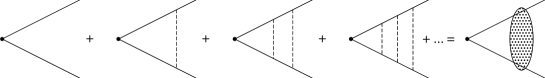
In perturbation theory, the first contribution to $\delta R^{+/0}$ is from the graphs in Fig. 1.

Figure 1: One-loop correction to $\Upsilon(4S)\to B\bar{B}$ due to (a) photon and (b) pion exchange.

The one-loop photon graph gives the $\pi\alpha/2v$ term in Eq. (2). It is enhanced by $\pi^{2}/v$ compared with a typical relativistic radiative correction, which is of order $\alpha/\pi$, because of the non-relativistic nature of the integral. The one-loop pion graph is similarly enhanced by $\pi^{2}/v\sim 150$ compared with a typical chiral loop correction. As a result, the correction from Fig. 1(b) is not small, and cannot be treated in perturbation theory. However, it is possible to sum the multiple pion exchanges by solving the Schrödinger equation using the one-pion plus one-photon exchange potential. This sums the series of graphs shown in Fig. 2.

Figure 2: Series of graphs summed by solving the Schrödinger equation. The dashed line represents pions and photons.

Additional corrections, such as vertex corrections, are not included in the Schrödinger equation. However, these corrections are not enhanced by $\pi^{2}/v$, and so are subleading compared with the terms we have retained.

The $H^{(b)}-H^{(\bar{b})}$ interaction potential is the same as the $H^{(b)}-H^{(b)}$ potential (by charge conjugation symmetry), and was computed in Ref. exotic which studied $bbqq$ exotic states. The potential depends on the $B^{*}B\pi$ coupling constant $g$ which is not known. Heavy quark symmetry implies that $g$ is the same as the $D^{*}D\pi$ coupling. The $D^{*}$ can decay into $D\pi$ (via the coupling $g$) or $D\gamma$ (via electromagnetic interactions), and the decay rates can be used to obtain $g$ amundson ; cho . A fit to the experimental data gives two possible solutions, $g=0.27\,^{+0.04}_{-0.02}\,{}^{+0.05}_{-0.02}$ or $g=0.76\,^{+0.03}_{-0.03}\,{}^{+0.2}_{-0.1}$ is , with the smaller value being preferred. A recent measurement of the $D^{*+}$ width by the CLEO collaboration gives $g=0.59\pm 0.01\pm 0.07$ gCLEO . We will give our results as a function of $g$.

The $\Upsilon(4S)$ is a $1^{--}$ state, and can decay into five possible channels, (i) $B\bar{B}$ with $S=0$, $\ell=1$, (ii) $B^{*}\bar{B}^{*}$ with $S=0$, $\ell=1$, (iii) $B^{*}\bar{B}^{*}$ with $S=2$, $\ell=1$, (iv) $B^{*}\bar{B}^{*}$ with $S=2$, $\ell=3$ and (v) $B\bar{B}^{*}+B^{*}\bar{B}$ with $S=1$, $\ell=1$, where $\ell$ is the orbital angular momentum and $S$ is the total spin. Since the $\Upsilon(4S)$ is below $BB^{*}$ and $B^{*}B^{*}$ threshold, only the first state is allowed as a final state, but all five states need to be included as intermediate states in the calculation. [The actual number of states is double this, since one has both charged and neutral channels.] Let $\eta,\beta=1-5$ denote one of the five possible $\ell S$ states and $a,b=1,2$ denote the charged and neutral sectors, respectively, so that a given channel is labeled by the index pairs $\eta a$ or $\beta b$. The radial Schrödinger equation has the potential

$$V^{\pi}_{\eta a,\beta b}(r)+V^{\gamma}_{\eta a,\beta b}(r)+V^{\ell}_{\eta a,\beta b}(r)+M_{\eta}\delta_{\eta\beta}\delta_{a,b}$$ (3)

where $V^{\pi}$ is the pion potential, $V^{\gamma}$ is the Coulomb potential, $V^{\ell}$ is the angular momentum potential, and $M_{\eta}$ is the contribution due to the $B^{*}-B$ mass difference, $\Delta m$,

$$M_{1}=0,\qquad M_{5}=\Delta m,$$

$$M_{2}=M_{3}=M_{4}=2\Delta m.$$ (4)

The $B^{0}-B^{+}$ mass difference is $0.33\pm 0.28$ MeV pdg , and will be neglected in our analysis. Note that a $B^{0}-B^{+}$ mass difference of $0.33$ MeV contributes about $0.05$ to $\delta R^{+/0}$ from the $p^{3}$ dependence of the phase space of the $P$-wave decay.

The angular momentum potential is

$$V^{\ell}_{\eta a,\beta b}(r) = {\ell_{\eta}(\ell_{\eta}+1)\over m_{B}r^{2}}\delta_{a,b}\delta_{\eta\beta}$$ (5)

where $\ell_{\eta}=(1,1,1,3,1)$ are the angular momenta of the various channels. The denominator is $m_{B}$ since $m_{B}/2$ is the reduced mass of the $B\bar{B}$. The Coulomb potential is

$$V^{\gamma}_{\eta a,\beta b}(r) = -{\alpha\over r}\delta_{\eta\beta}\delta_{a1}\delta_{b1},$$ (6)

where $\alpha$ is the fine-structure constant. It only contributes to the charged sector $a=b=1$, and does not mix different $\ell S$ states.

The pion potential can be computed using the techniques given in Ref. exotic ; largen ; ej :

$$V^{\pi}_{\eta a,\beta b}(r) = \left[\begin{array}[]{cc}h_{+}^{2}U_{\eta\beta}\left(m_{\pi^{0}},r\right)&2U_{\eta\beta}\left(m_{\pi^{+}},r\right)\\ 2U_{\eta\beta}\left(m_{\pi^{+}},r\right)&h_{0}^{2}U_{\eta\beta}\left(m_{\pi^{0}},r\right)\end{array}\right]_{ab}$$ (9)

where $h_{+}^{2}=1.01$, $h_{0}^{2}=0.99$ ej . The structure of the potential is easy to understand. The off-diagonal elements are transition amplitudes between the charged and neutral sectors due to $\pi^{+}$ exchange, and depend on the charged pion mass $m_{\pi^{+}}$ and coupling constant $g$, which is included in the definition of $U$. The diagonal matrix elements are due to $\pi^{0}$ exchange, and depend on $m_{\pi^{0}}$. In the absence of $\eta-\pi^{0}$ mixing, the $\pi^{+}$ coupling constant is $\sqrt{2}$ time the $\pi^{0}$ coupling which gives the $2:1$ ratio of the off-diagonal to diagonal elements. The values of $h_{+}$ and $h_{0}$ differ from unity due to $\eta-\pi^{0}$ mixing ej .

The computation of the matrix $U_{\eta\beta}(m_{\pi},r)$ is non-trivial. The answer is that

$$U(m,r)=T\,\widetilde{U}(m,r)\,T^{t}$$ (10)

where

$$\tilde{U}(m,r) = {g^{2}m^{2}e^{-mr}\over 8\pi f^{2}r}\left[\begin{array}[]{ccccc}1&0&0&0&0\\ 0&u_{1}&0&0&0\\ 0&0&u_{2}&0&0\\ 0&0&0&u_{2}&0\\ 0&0&0&0&u_{1}\end{array}\right],$$ (16)

$$u_{1}(m,r) = \left(1+{2\over mr}\right)^{2},$$

$$u_{2}(m,r) = -\left(1+{2\over mr}+{2\over m^{2}r^{2}}\right),$$ (17)

$f\sim 132$ MeV is the pion decay constant and

$$T=\left(\begin{array}[]{ccccc}{1\over 2}&-{1\over 2}&0&{1\over\sqrt{2}}&0\\ {\sqrt{3}\over 2}&{1\over 2\sqrt{3}}&0&-{1\over\sqrt{6}}&0\\ 0&-{2\over\sqrt{15}}&-\sqrt{3\over 10}&-\sqrt{2\over 15}&-\sqrt{3\over 10}\\ 0&\sqrt{2\over 5}&-{1\over\sqrt{5}}&{1\over\sqrt{5}}&-{1\over\sqrt{5}}\\ 0&0&-{1\over\sqrt{2}}&0&{1\over\sqrt{2}}\end{array}\right),$$ (23)

and $T^{t}$ is the transpose of $T$.

Equation (9) is the leading contribution to the long distance part of the potential. As argued in Ref. exotic , Eq. (9) will dominate the potential until $r\sim 1/(2m_{\pi})$ at which point two-pion exchange begins to contribute. We introduce a cutoff $r_{\text{min}}=1/(2m_{\pi})$, and use Eq. (9) for $r\geq r_{\text{min}}$, and set $V^{\pi}=0$ for $r<r_{\text{min}}$. The short distance part of the potential can be included into a renormalization of the production vertex. The Coulomb potential will be allowed to act until $r=0$.

The $\Upsilon(4S)$ is produced by the space component of the electromagnetic current $\bar{b}\gamma^{i}b$. Heavy quark spin symmetry holds in the $\Upsilon$ system falk ; Bc , so the $\Upsilon(4S)$ decays into $H^{(b)}-H^{(\bar{b})}$ such that the spins of the heavy quarks in the final mesons are combined to form the spin of the $\Upsilon(4S)$, i.e. the polarization of the virtual photon. The orbital angular momentum and spin of the light degrees of freedom are combined to form total angular momentum zero. A little Clebsch-Gordan algebra shows that the amplitude for the $\Upsilon(4S)$ to decay into the five channels is falk

$$A_{\eta a}=c_{a}\left({1\over 2\sqrt{3}},-{1\over 6},{\sqrt{5}\over 3},0,-{1\over\sqrt{3}}\right)_{\eta}\ .$$ (24)

The amplitude for decay to the $\ell=3$ channel is zero to this order in the velocity expansion. The coefficients $c_{a},\ a=1,2$ are unknown, but the absolute values of $c_{a}$ are irrelevant for the computation of $R^{+/0}$; all that is needed is the ratio $c_{1}/c_{2}$ of the charged to neutral production amplitudes. The dominant production of the $B$ mesons is via the isosinglet $\Upsilon(4S)$ state, in which case $c_{1}=c_{2}$. Isospin violating effects, including direct production of $B$’s not via the $\Upsilon(4S)$ lead to a deviation of $c_{1}/c_{2}$ from unity. As discussed above, cutoff effects in the potential can be absorbed into the production amplitudes $c_{a}$. One expects short-distance corrections to introduce isospin violation in the ratio $c_{1}/c_{2}$ of a few percent, the typical size of other isospin violating effects in hadron physics. We will define $\delta c$ by $c_{1}/c_{2}=1+\delta c$. The value of $\delta c$ is related to the value of $r_{\text{min}}$, since changes in the cutoff induce changes in the Lagrangian coefficients. Since $\delta c$ is unknown, our computation of $R^{+/0}$ is uncertain at the 5% level; however the uncertainity is much smaller than the expectation that $\delta R^{+/0}$ is 19% from Coulomb interactions alone. Cutting off the Coulomb potential at short distances reduces the value of $\delta R^{+/0}$. Since the Coulomb potential is the dominant source of isospin violation, one expects that $\delta c$ will be negative.

The method of computation is as follows. One solves the Schrödinger equation with potential Eq. (9). The boundary condition on the wavefunction as $r\to\infty$ is that one has a plane wave plus an outgoing scattered wave. [One can see this directly from the sum of graphs in Fig. 2.] Only the $B^{+}B^{-}$ and $B^{0}\bar{B}^{0}$ states exist as propagating modes as $r\to\infty$; the other channels have exponentially decaying wavefunctions. The plane wave state is chosen to be in the $B^{+}B^{-}$ or $B^{0}\bar{B}^{0}$ channels to compute the charged or neutral meson production rates, respectively. The overlap of the computed wavefunction as $r\to 0$ with the production amplitude Eq. (24) gives the final production amplitude, the absolute square of which gives the production rate. [Note that the wavefunction near $r=0$ can have all five channels.] The answer for $R^{+/0}$ depends on $\delta c$, $g$ and the velocity $v$ of the outgoing $B$ meson. Provided the dominant production mechanism is via the photon coupling to the heavy quark, the result for $R^{+/0}$ holds even away from the $\Upsilon(4S)$ resonance since it depends only on the quarks being non-relativistic. The value of $c_{a}$ will depend strongly on the beam energy, and peak at the resonance, but $\delta c$, the isospin violation in the production amplitude should be a smooth function of energy.

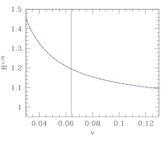
In Fig. 3 we have plotted $R^{+/0}$ as a function of $g$ for $\delta c$ and $v=0.064$, the value in $\Upsilon(4S)$ decay.

Figure 3: $R^{+/0}$ as a function of $g$ for $v=0.064$ and $\delta c=0.02$ (dotted), $0.0$ (solid), $-0.02$ (dashed) and $-0.04$ (dot-dashed).

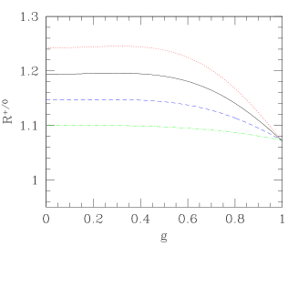
$R^{+/0}$ is approximately constant and equal to its value from only Coulomb corrections, Eq. (9), until $g>0.6$, at which point $R^{+/0}$ starts to decrease. $R^{+/0}$ is approximately constant for small $g$ even though the shifts in the production amplitudes are large. The one-loop pion graph in Fig. 1 is about three times the tree-level graph. Summing the pion graphs in Fig. 2 gives about a 20% (for $g\sim 0.6$) shift in the charged and neutral production rates. The rates into the charged and neutral channels vary by about a factor of two for the range of Yukawa couplings in Fig. 3, but their ratio $R^{+/0}$ varies by about 10%. For larger values of $g$ than those shown, $R^{+/0}$ has rapid $v$ dependence due to the formation of meson bound states, because the pion-exchange potential is sufficiently attractive. For our choice of parameters, this occurs for $g\sim 1.3$, well outside the allowed range is ; gCLEO .

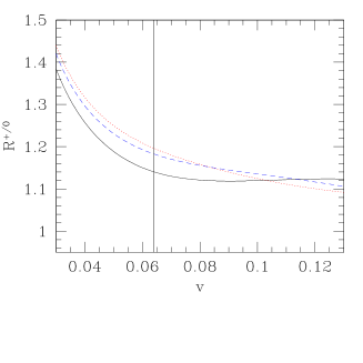
In Fig. 4 and 5, we have plotted $R^{+/0}$ as a function of velocity for different values of $\delta c$ for two illustrative choices $g=0.3$ and $g=0.8$ consistent with the two solutions for $g$ found in Ref. is . The vertical line is the velocity at the $\Upsilon(4S)$.

Figure 4: $R^{+/0}$ as a function of $v$ for $g=0.3$ and $\delta c=0.02$ (dotted), $0.0$ (solid), $-0.02$ (dashed) and $-0.04$ (dot-dashed).

Figure 5: $R^{+/0}$ as a function of $v$ for $g=0.8$ and $\delta c=0.02$ (dotted), $0.0$ (solid), $-0.02$ (dashed) and $-0.04$ (dot-dashed).

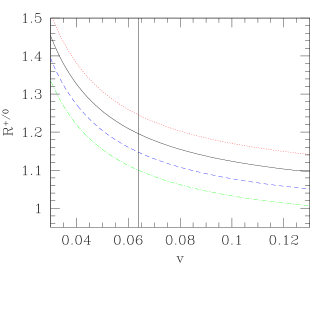
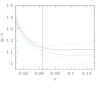
At the $\Upsilon(4S)$ peak, for $g=0.8$, $R^{+/0}$ varies from $1.17$ to about $1.09$, whereas for $g=0.3$, $R^{+/0}$ varies between about $1.25$ and $1.1$.

In Figs. 6 and 7, we have plotted $R^{+/0}$ as a function of $v$ for $g=0.3$ and $g=0.8$, respectively, for different values of the cutoff from $r_{\text{min}}=1/(2m_{\pi})$ to $1/m_{\pi}$. For small values of $g$, the variation of the cutoff does not change $R^{+/0}$. For larger values of $g$, the cutoff variation is consistent with expectations from naive dimensional analysis amhg . A factor of two variation in the cutoff introduces a $4\%$ variation in $R^{+/0}$.

Figure 6: $R^{+/0}$ as a function of $v$ for $g=0.3$, $\delta c=0$, and cutoffs $r_{\text{min}}=1/(2m_{\pi})$ (solid), $1/\sqrt{2}m_{\pi}$ (dashed), $1/m_{\pi}$ (dotted).

Figure 7: $R^{+/0}$ as a function of $v$ for $g=0.8$, $\delta c=0$, and cutoffs $r_{\text{min}}=1/(2m_{\pi})$ (solid), $1/\sqrt{2}m_{\pi}$ (dashed), $1/m_{\pi}$ (dotted).

The absolute value of $R^{+/0}$ depends on the value of $\delta c$, and the cutoff $r_{\text{min}}$. If $g$ is small ($\sim 0.3$, the preferred value in Ref. is ), then for values of $\delta c$ consistent with expectations from dimensional analysis, one expects $\delta R^{+/0}\gtrsim 0.1$. The Yukawa corrections do not significantly change $R^{+/0}$ from the Coulomb value. We note, however, that this is due to a cancellation in $R^{+/0}$ after summing the graphs in Fig. 2; the one loop pion correction from Fig. 1 is about three, and is not small. If $g$ is close to the larger value $g=0.8$, then $\delta R^{+/0}$ at the $\Upsilon(4S)$ is smaller, but still around $0.1$. In this case, there is some cutoff dependence, so $R^{+/0}$ is more uncertain.

The dependence of $R^{+/0}$ on $v$ (or equivalently, $\sqrt{s}$) is calculable. One can see that the curves in Fig. 4 have a different shape from those in Fig. 5, so measuring $R^{+/0}$ as a function of $v$ can provide information on the $B^{*}B\pi$ and $D^{*}D\pi$ coupling $g$, which is needed for many calculations, such as the ratio of the $B_{s}-\bar{B}_{s}$ to $B-\bar{B}$ mixing amplitudes gjmsw .