Abstract

We propose to measure the $CP$ phase $\delta_{\rm CP}$, the magnitude of the neutrino mixing matrix element $|U_{e3}|$ and the sign of the atmopheric scale mass–squared difference $\Delta{\rm m}^{2}_{31}$ with a superbeam by the joint analysis of two different long baseline neutrino oscillation experiments. One is a long baseline experiment (LBL) at 300 km and the other is a very long baseline (VLBL) experiment at 2100 km. We take the neutrino source to be the approved high intensity proton synchrotron, HIPA. The neutrino beam for the LBL is the 2-degree off-axis superbeam and for the VLBL, a narrow band superbeam. Taking into account all possible errors, we evaluate the event rates required and the sensitivities that can be attained for the determination of $\delta_{\rm CP}$ and the sign of $\Delta m^{2}_{31}$. We arrive at a representative scenario for a reasonably precise probe of this part of the neutrino physics.

I Introduction

The Super-Kamiokande experiments [1] in the past several years, joined by SNO [2] more recently, have given strong indications of neutrino oscillation that are corroborated and constrained by a variety of other experiments. These experiments started a new era in the study of neutrino physics and offered the best indication to date of physics beyond the standard model. To further probe neutrino physics, there are a number of ongoing and planned neutrino oscillation experiments. These experiments promise to give a full description of the phenomenology of neutrino mixing. The most attractive experiments among the new generation of neutrino oscillation experiments are the long baseline (LBL) experiments. They are performed in the controlled environment of traditional experimental high energy physics and expected to allow precision measurements of the oscillation parameters, including the leptonic $CP$ phase. Notably, the recently approved superbeam facility, the High Intensity Proton Accelerator (HIPA) [3], which can provide intensive high energy neutrino beams from its 50 GeV proton synchrotron, offers the possibility of even more desirable LBL experiments. So far, the possibility of two LBL experiments using the HIPA superbeam have been discussed. One is HIPA to Kamiokande at a baseline length of about 300 km  [4] known as J2K, and the other is HIPA to a detector located 2100 km away near Beijing [5, 6] called H2B. It is well-known that there are parameter ambiguities that are generally associated with oscillation measurements at a single baseline[7, 8]. Measurements at more than one baseline can be beneficial [6, 9, 10]; our previous studies [11, 12] showed that the joint analysis of the J2K and H2B experiments can offer extra leverages to resolve some of these ambiguities. Our results, however, also showed that $CP$ violation effects cannot be determined at 3$\sigma$ level even with the joint analysis considered in the study, in which no antineutrino beams were used.

Since the leptonic $CP$ phase and mass–squared difference sign are pertinent information in the physics of neutrino mixings, which seems to be very different from that of the quark sector, it is necessary to find out how to pin down these neutrino mixing parameters accurately in new experiments. It has been widely recognized that the neutrino factory [13] is an ideal facility for the study of neutrino mixings. However, because of the technical and budgetary challenges faced with building a workable neutrino factory in the near future, and because of the availability of a conventional superbeam from HIPA in about five years, it is obviously advisable that we explore the full potential of the HIPA superbeams. In this work, we examine in further detail the measurement of the $CP$ phase and the mass–squared difference sign from the joint analysis at the two long baselines with specific HIPA superbeams and more suitable detectors. The neutrino beams are the 2-degree off-axis superbeams for the LBL at 300 km and a narrow band superbeam for VLBL at 2100 km. We evaluate the event rates and investigate their sensitivities to the $CP$ phase and the sign of $\Delta m^{2}_{31}$. Taking into account all possible experimental errors, we find that a fairly precise measurement of the $CP$ phase, the sign of the mass–squared difference and the mixing angle $\theta_{13}$ is possible but requires: (1) the joint analysis at the two baselines; (2) that both a $\nu_{\mu}$ beam and a $\bar{\nu}_{\mu}$ beam are needed at 300 km; (3) that a $\bar{\nu}_{\mu}$ beam is needed at 2100 km if $\Delta m^{2}_{31}$ is negative; and (4) a significant increase in the statistics at both 300 km and 2100 km. We find that $\sin^{2}(2\theta_{13})$ can be probed to very small values, depending on the value of the $CP$ phase.

In Sec. II we describe how the simulations are performed. In Sec. III our results are presented. A brief discussion and conclusion can be found in Sec. IV.

II Description of simulations

A Parametrization and inputs

Our oscillation analyses will be restricted to 3 flavors of active neutrinos. The parameters of the system consists of 2 mass–squared differences (MSD), 3 mixing angles and 1 measurable $CP$ phase. The unitary mixing matrix in the vacuum is parameterized as usual

$$U = \left(\begin{array}[]{ccc}c_{12}c_{13}&c_{13}s_{12}&\hat{s}^{*}_{13}\\ -c_{23}s_{12}-c_{12}\hat{s}_{13}s_{23}&c_{12}c_{23}-s_{12}\hat{s}_{13}s_{23}&c_{13}s_{23}\\ s_{12}s_{23}-c_{12}c_{23}\hat{s}_{13}&-c_{12}s_{23}-c_{23}s_{12}\hat{s}_{13}&c_{13}c_{23}\end{array}\right),$$ (4)

where $s_{jk}=\sin(\theta_{jk})$, $c_{jk}=\cos(\theta_{jk})$, and $\hat{s}_{jk}=\sin(\theta_{jk})e^{i\delta_{\rm CP}}$, $\theta_{jk}$ defined for $j<k$ are the mixing angles of mass eigenstates $\nu_{j}$ and $\nu_{k}$, and $\delta_{\rm CP}$ is the $CP$ phase angle. The three mass eigenvalues are denoted as $m_{1}$, $m_{2}$, and $m_{3}$. The two independent MSD are $\Delta{\rm m}^{2}_{21}\equiv{\rm m}^{2}_{2}-{\rm m}^{2}_{1}$ and $\Delta{\rm m}^{2}_{31}\equiv{\rm m}^{2}_{3}-{\rm m}^{2}_{1}$.

The inputs of the mixing angles and MSD’s are obtained from solar, atmospheric and reactor experiments:

$$\sin^{2}(2\theta_{12})=0.8, ~{}~{}~{}\Delta{\rm m}^{2}_{21}=5\times 10^{-5}{\rm eV}^{2},$$ (5)

$$\sin^{2}(2\theta_{23})=1.0, ~{}~{}~{}|\Delta{\rm m}^{2}_{31}|=3\times 10^{-3}{\rm eV}^{2},$$ (6)

$$\sin^{2}(2\theta_{13})\leq 0.1.$$ (7)

Note that the sign of $\Delta m^{2}_{31}$ is unknown. The currently favored Large Mixing Angle solar solution requires $\delta m^{2}_{21}>0$.

In LBL experiments the neutrino beam interacts with electrons contained in Earth matter [14]. In the present study we use the Preliminary Reference Earth Model [15], generally known as PREM, for Earth density profiles [16] and numerically integrate the Schrödinger equation that descibes the propagation of the neutrino in matter for the treatment of distance dependent matter density. However, we note that there exist more sophisticated approaches to Earth matter effect, including both an updated average density profile known as the AK135 [17] and treatments of uncertainties of the density profile [8, 18, 19] which can affected the determination of the $CP$ phase angle.

B Beams and detectors

The HIPA 50 GeV proton synchrotron beam calls for a power of 0.77 MW in phase I, to be upgraded to 4 MW in phase II. The superbeam provided by HIPA can be a wide band beam (WBB), a pulsed narrow band beam (NBB), or an off-axis beam (OAB). The WBB contains neutrinos with widely distributed energy. In a NBB the neutrino flux is concentrated in a narrow range of energies, with maximum energy $E_{\rm peak}$ where the intensity is peaked, and the intensity decreases rapidly below $E_{\rm peak}$. An OAB also peaks at a certain energy, but has a longer high-energy tail than that of a NBB. More details of the various beam profiles can be found in Ref. [20]. For the 2100 km baseline we use a NBB [21] with peak energy of 4 GeV. We have also investigated the beams of peak energies of 5, 6 and 8 GeV, but found that the 4 GeV beam gives the best results. For 300 km we use the 2-degree OAB (2^∘–OAB) which has a peak energy at 0.8 GeV [22].

The detector at 2100 km is assumed to be a water Cerenkov calorimeter with resistive plate chambers [23, 5] located in Beijing, tentatively called the Beijing Astrophysics and Neutrino Detector (BAND). The size of the detector will be 100 kt at the beginning and can be upgraded to a much larger one depending on the physics requirements. The detector at 300 km is initially the Kamiokande detector of the present size of 22.5 kt and upgraded later to 450 kt.

C Experimental errors

For the experimental errors we use 3$\sigma$ throughout this work. All independent errors, statistical and systematic, are added in quadrature. For the statistical error we used $3\sigma$ Poisson errors as described in the appendix of Ref. [24], including a background at the 1% level of the rate of the survival channel. For the systematic error we assumed that the background is known at the 2% level as given in  [25]. To estimate the error due to the uncertainty in the measurement of the mixing angle $\theta_{23}$, we assumed that $\sin^{2}(2\theta_{23})$ is measured via the survival channel at $L=300$ km, with the event rate given by $N(\nu_{\mu}\to\nu_{\mu})\simeq N_{0}(1-\sin^{2}(2\theta_{23})\sin^{2}(\Delta))$, where $\Delta\simeq\pi/2$ and $N_{0}$ is the number of events in the absence of oscillations. Then the statistical uncertainty on $\sin^{2}(2\theta_{23})$ is

$$\delta(\sin^{2}(2\theta_{23}))=\sqrt{N}/N_{0}\approx{1\over\sqrt{N_{0}}}\sqrt{(1-\sin^{2}(2\theta_{23})\sin^{2}(\Delta))}\,.$$ (8)

We then find the variation in the rate in question for a 3$\sigma$ deviation in $\theta_{23}$, and added this in quadrature to the other 3$\sigma$ errors described above to obtain the total 3$\sigma$ error.

D Scenarios

We consider three scenarios in the present investigation. The scenarios are summarized in Table 1. For Scenario I the first stage involves a 5-year experiment with a water Cerenkov detector of 22.5 kt at 300 km with the 2^∘–OAB $\nu_{\mu}$ beam [22] from HIPA at 0.77 MW. This stage is contained in the plan of J2K [4]. The second stage of this scenario has HIPA upgraded to 4 MW, as discussed in Ref. [5], to deliver a NBB $\nu_{\mu}$ beam to the water Cerenkov detector of 100 kt at L=2100 km to run for 5 years.

Scenario II has an upgraded 4 MW HIPA and calls for both $\nu_{\mu}$ and $\bar{\nu}_{\mu}$ beams. The experiment at 2100 km is the same as in Scenario I. For 300 km, however, we assume a much larger water Cerenkov detector of 450 kt. It will run for 2 years with 2^∘–OAB $\nu_{\mu}$ beam, and then 6 years with the 2^∘–OAB $\bar{\nu}_{\mu}$ beam.

Scenario III is similar to Scenario II, but calls for a much larger water Cerenkov detector at 2100 km, to run either the $\nu_{\mu}$ or $\bar{\nu}_{\mu}$ beam, for example, for 5000 kt-yr. Whether a $\nu$ or $\bar{\nu}_{\mu}$ beam is delivered to the 2100 km site depends on the sign of $\Delta{\rm m}^{2}_{31}$, as will be explained below.

III Results of the simulation

A Strategy

Let us first describe briefly the strategy of our calculation. There are 6 measurable oscillation parameters in the 3-flavor neutrino scheme. There are two mass scales; one is the atmospheric scale and the other the solar scale. Existing oscillation experiments have determined that the two mass scales are widely separated and therefore sensitive to different $L/E_{\nu}$ regions. The LBL and VLBL we are considering are affected by the solar scale only at next–to–leading order, but can be strongly affected by the unknown parameters $\delta_{CP}$ and $\theta_{13}$. Hence we will take $\Delta{\rm m}^{2}_{21}$ and $\theta_{12}$ to be the values determined in solar experiments, as given in Eq. (5). This leaves 4 parameters to be determined, but $|\Delta{\rm m}^{2}_{31}|$ and $\theta_{23}$ are known already to a fair degree of accuracy from atmospheric neutrino experiments. Therefore obtaining $\theta_{13}$, $\delta_{\rm CP}$, and the sign of $\Delta{\rm m}^{2}_{31}$ is the main goal of our calculation.

The current and soon to be online LBL experiments will determine $|\Delta{\rm m}^{2}_{31}|$ and $\sin^{2}(2\theta_{23})$ to a better accuracy; $\delta m^{2}_{21}$ and $\sin^{2}(2\theta_{12})$ will be measured more precisely by KamLAND [26, 27]. The first task of the scenarios we propose is to determine $|\Delta{\rm m}^{2}_{31}|$ and $\sin^{2}(2\theta_{23})$ more accurately, using the $\nu_{\mu}$ survival probability. This will allow us to have as small an uncertainty as possible in the determination of the parameters $\theta_{13}$ and $\delta_{CP}$. Let us define $N_{\alpha}(L)$ as the number of charge–current events involving the $\alpha$ charged lepton at the baseline $L$. We assume that $N_{\mu}(300)$, which depends on the $\nu_{\mu}$ survival probability, is used to determine $|\Delta m^{2}_{31}|$ and $\theta_{23}$ with as small an error as possible. Then in the various scenarios $N_{\mu}(300)$ cannot be used to determine $\theta_{13}$ and $\delta_{CP}$. 

B Scenario I ($\nu_{\mu}$ beam only)

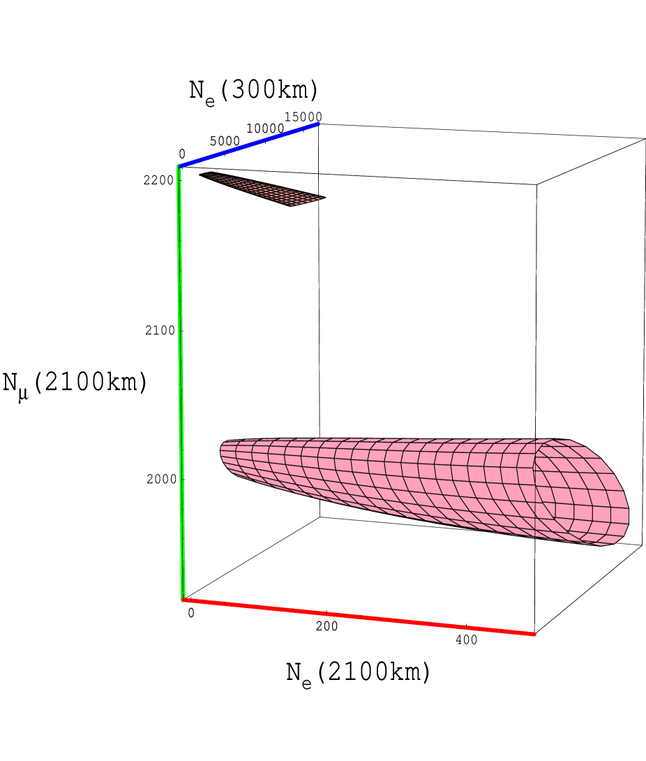
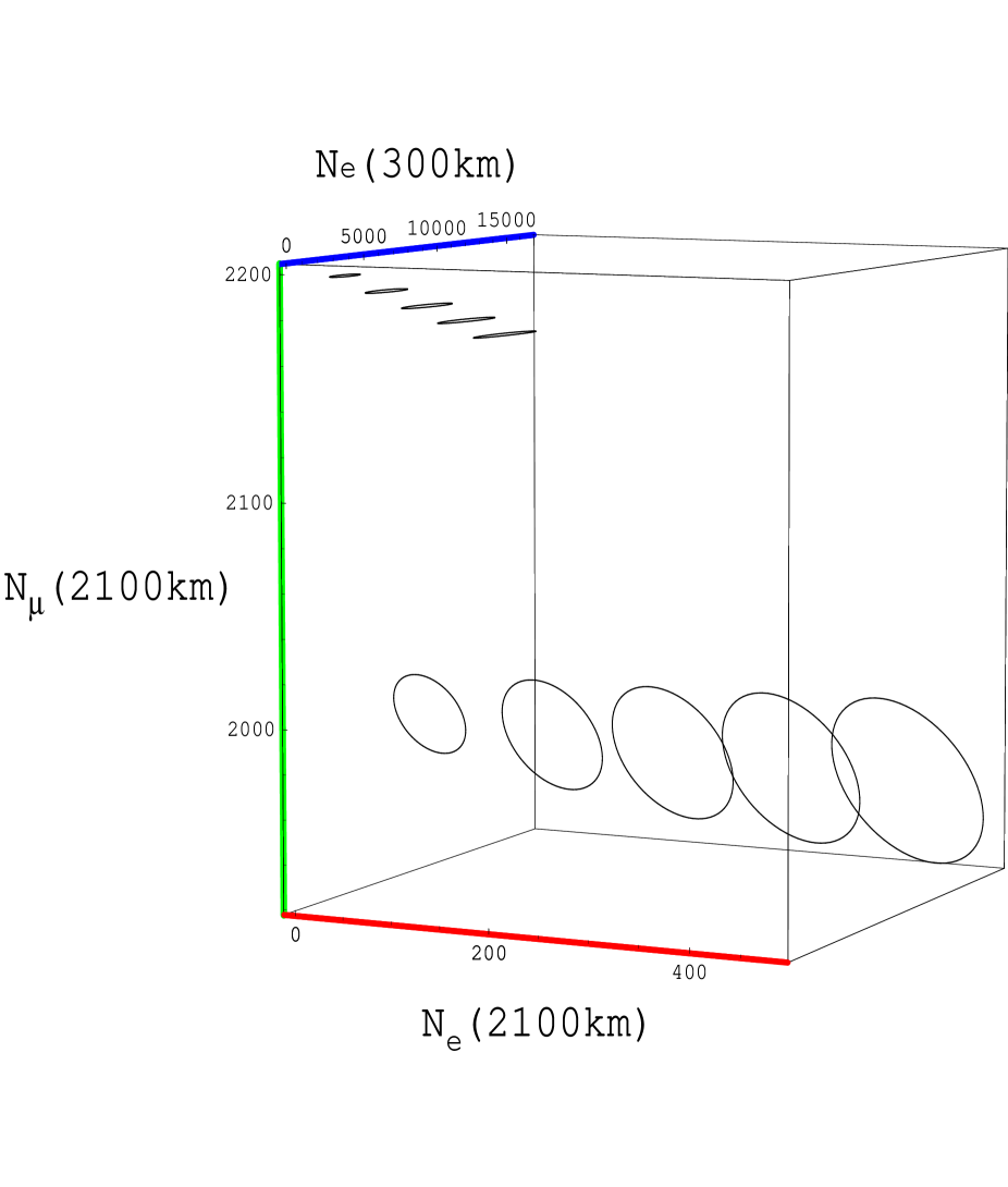
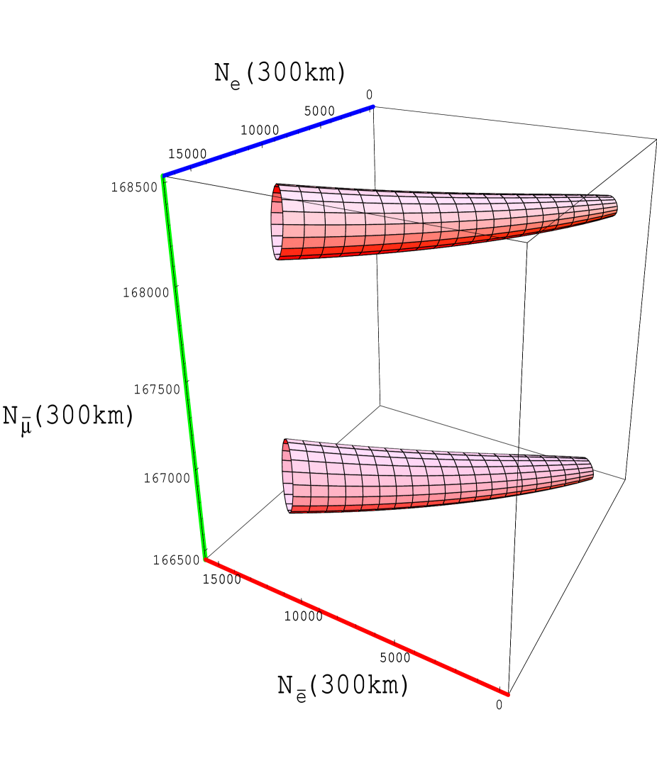
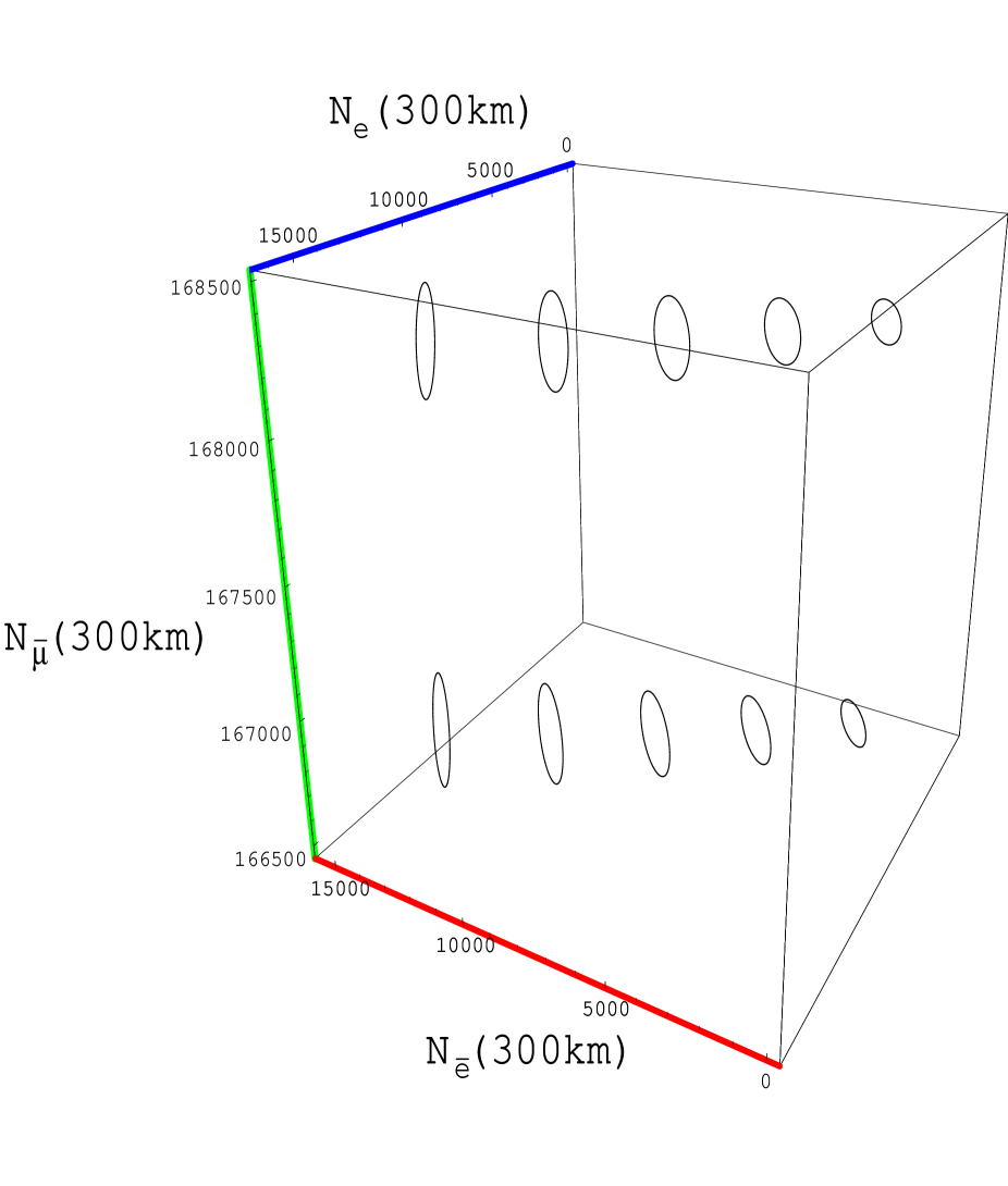
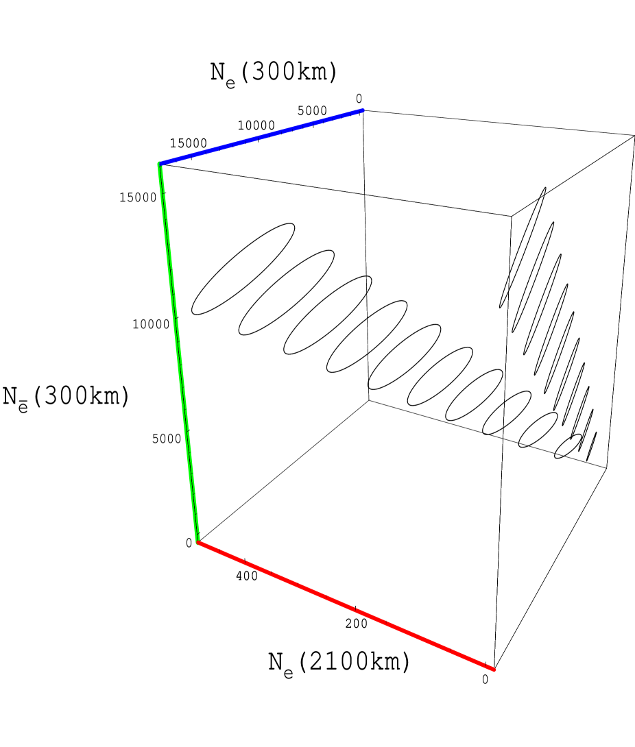
In this scenario we assume that only the $\nu_{\mu}$ beam is employed to run at $L$=300 km and 2100 km. Since $N_{\mu}(300)$ has already been used to determine $|\Delta m^{2}_{31}|$ and $\sin^{2}(2\theta_{23})$, we are left with three types of independent measurements for the determination of $\theta_{13}$, $\delta_{\rm CP}$ and the sign of $\Delta m^{2}_{31}$: $N_{e}(300)$, $N_{e}(2100)$ and $N_{\mu}(2100)$. The measurements of these three types of events form a surface in a three-dimensional space when $\theta_{13}$ and $\delta_{CP}$ are varied in their allowed ranges. The angle $\theta_{13}$ is constrained by the CHOOZ reactor experiment [28] and the $CP$ phase is completely unconstrained. Therefore, we take their ranges to be: $\sin^{2}(2\theta_{13})=(0,0.1)$ and $\delta_{\rm CP}=(0,2\pi$). Such three–dimensional surfaces, which are tube–like, are displayed in Fig. 1. The upper and lower surfaces are for negative and positive $\Delta{\rm m}^{2}_{31}$, respectively. The closed curves around the axes of the tubes are traced out by varying $\delta_{\rm CP}$ from $0$ to $2\pi$, while the lines running parallel to the axes of the tubes are determined by varying $\sin^{2}(2\theta_{13})$ from $0.01$ to $0.1$. For fixed $\sin^{2}(2\theta_{13})$ values, we then obtain the ellipses in Fig. 2.

When $N_{e}(300)$, the number of the $\nu_{e}$ appearance events at 300 km, is measured, it determines a closed curve which is obtained from the three-dimensional surface by a cut at a given value on the $N_{e}(300)$ axis. The value of $N_{e}(300)$ does not determine $\theta_{13}$ directly since $\delta$ is unknown; for each of the closed curves we obtain a definite relation between $\delta$ and $\sin^{2}(2\theta_{13})$ when the sign of $\Delta m^{2}_{31}$ is given. We show in Fig. 3 two sets of such relations for each $\Delta{\rm m}^{2}_{31}$ sign. As shown, we choose two extreme values of $N_{e}(300)$, each of which leads to a range of values for $\sin^{2}(2\theta_{13})$, depending on the sign of $\Delta{\rm m}^{2}_{31}$. For positive $\Delta{\rm m}^{2}_{31}$, the larger $N_{e}(300)$ curve limits $\sin^{2}(2\theta_{13})$ to the range ($0.06,0.1$), while the smaller one corresponds to $\sin^{2}(2\theta_{13})$ lying in the range ($0.006,0.01$). Similarly, the ranges of the values of $\sin^{2}(2\theta_{13})$ for negative $\Delta{\rm m}^{2}_{31}$ can be read off from Fig. 3.

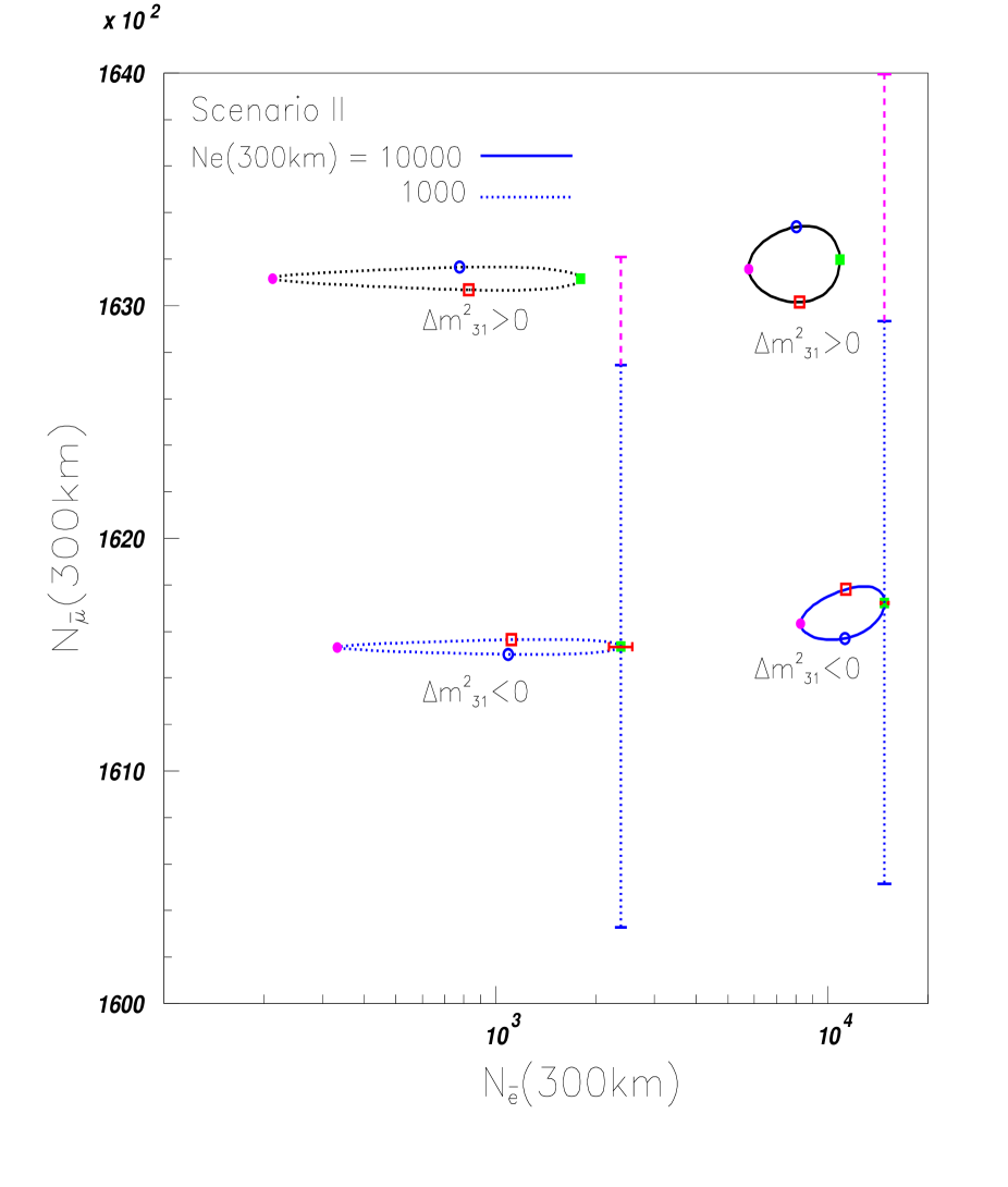
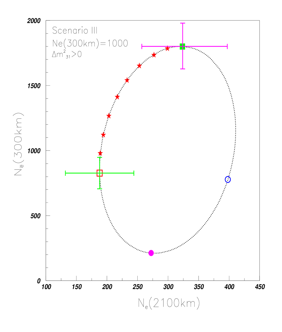
We plot in Fig. 4 the two-dimensional curves with fixed $N_{e}(300)$. Note that the scale of the horizontal axis is logarithmic. If the scale was linear, the curves would be ellipses. An open square indicates the point on a curve with $\delta_{\rm CP}$=0^∘, solid square 90^∘, open circle 180^∘, and solid circle 270^∘. We also show a representative 3$\sigma$ error bar for each curve. The assignment of statistical and systematic errors has been discussed in the preceding section. The total error is dominated mostly by the statistical error. One sees that although the sign of $\Delta m^{2}_{31}$ can be determined at the 3$\sigma$ level, there is no sensitivity to the value of the $CP$ phase. In particular, the error in the $N_{\mu}(2100)$ channel is very large in comparison with the range of variation in the number of events when $\delta_{\rm CP}$ varies; we will encounter similar situation in the next scenario.

C Scenario II ($\nu$ and $\bar{\nu}$ beams)

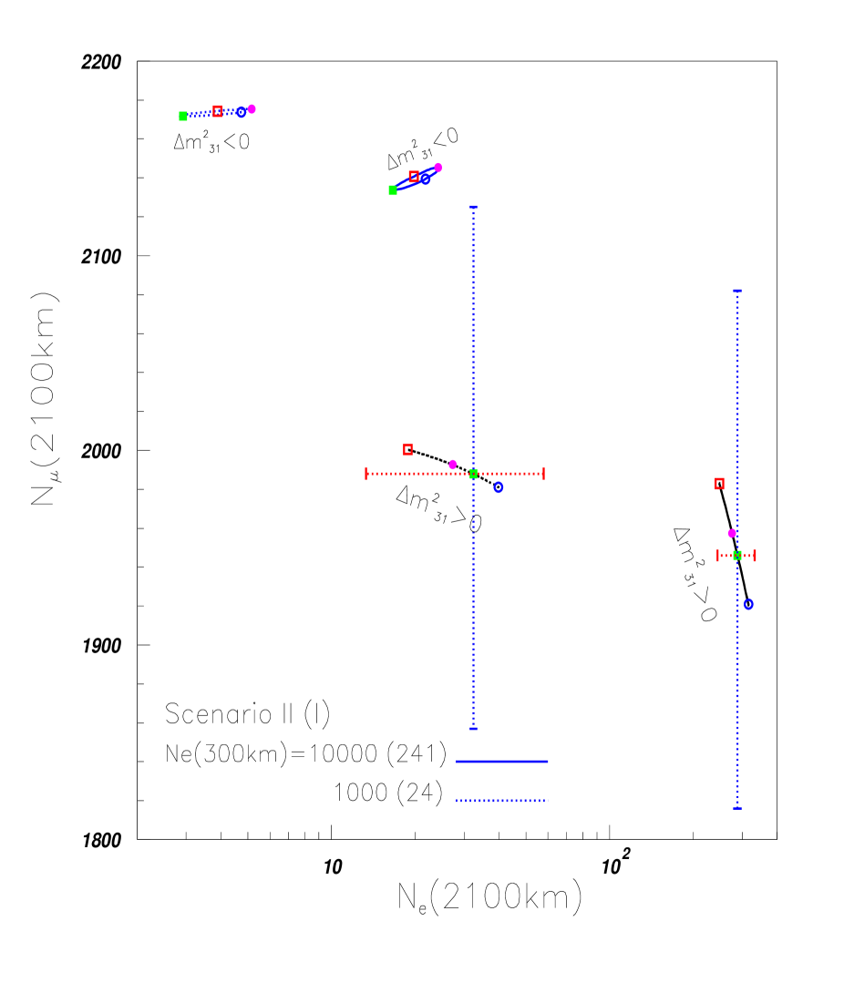
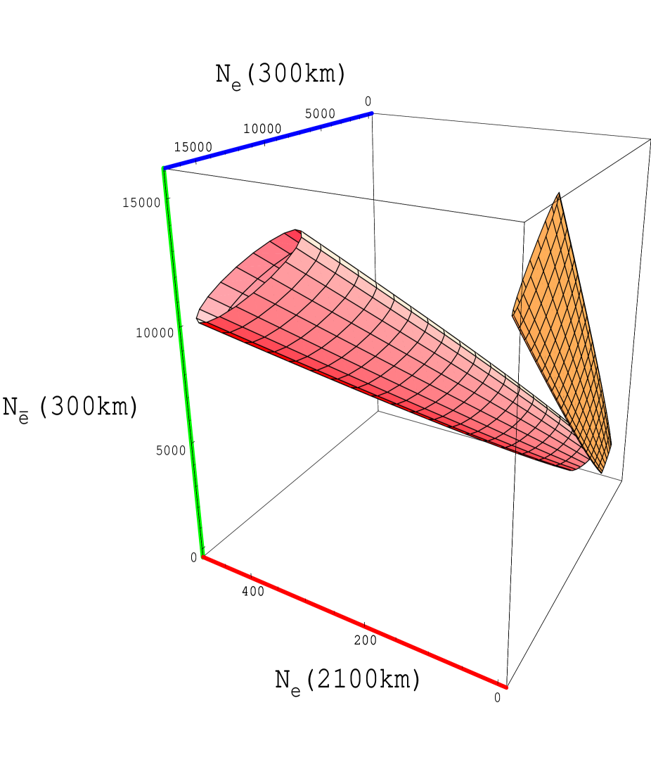
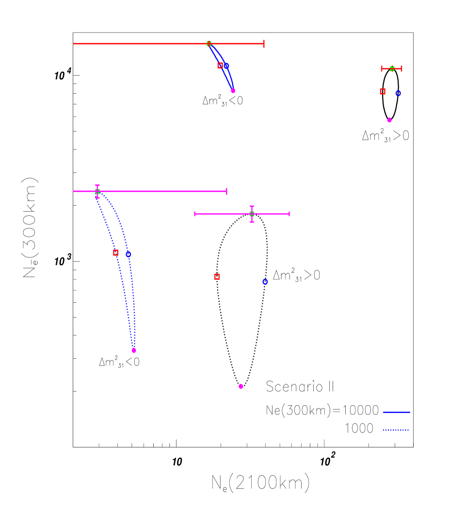
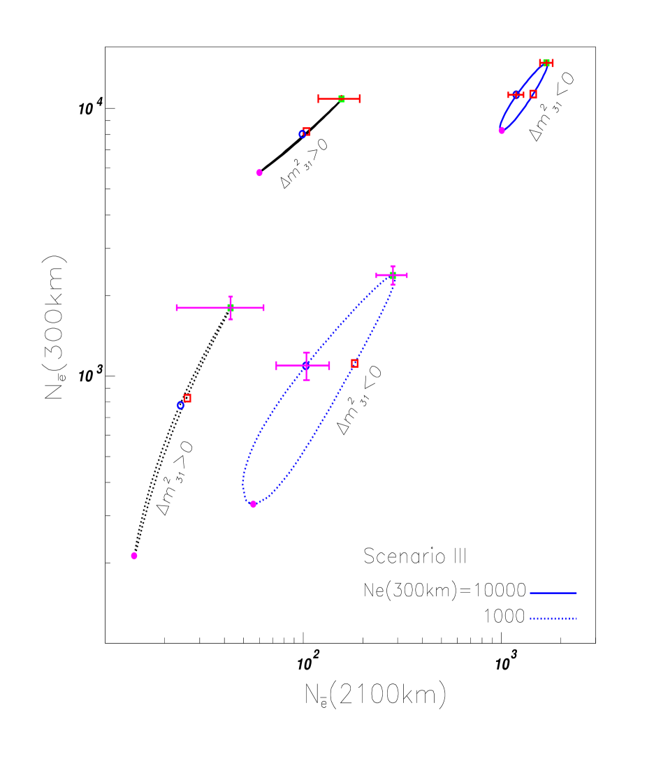
By including the $\bar{\nu}_{\mu}$ beam aimed at the detector at 300 km, we have two more types of events, i.e., $N_{\bar{e}}(300)$ and $N_{\bar{\mu}}(300)$. So, in addition to the three-dimensional surface in the $N_{e}(300)$-$N_{e}(2100)$-$N_{\mu}(2100)$ space shown earlier in Fig. 1, we also have surfaces in the spaces $N_{e}(300)$-$N_{\bar{e}}(300)$-$N_{\bar{\mu}}(300)$ and $N_{e}(300)$-$N_{\bar{e}}(300)$-$N_{e}(2100)$, as shown in Figs. 5 and 8, respectively. With several fixed values of $\sin^{2}(2\theta_{13})$ we obtain the curves shown in Figs. 6 and 9. We plot the two-dimensional projections of fixed $N_{e}(300)$=1000 and 10000 in Figs. 7 and 10.

We found in Scenario I that the 2100 km data with just a $\nu_{\mu}$ source can determine the sign of $\Delta m^{2}_{31}$ at 3$\sigma$, but cannot measure the $CP$ phase (see Fig. 4). In contrast, as shown in Fig. 7, the 300 km data using both a $\nu$ and $\bar{\nu}$ source can determine the $CP$ phase in the ranges ($\pi/2,3\pi/2$) or ($-\pi/2,\pi/2$), but cannot distinguish between the two ranges since the measurement is only sensitive to $\sin\delta$. Furthermore, unless $\delta_{CP}$ is close to $\pi/2$ or $3\pi/2$ the sign of $\Delta m^{2}_{31}$ cannot be determined once all of the experimental errors, including the error in the determination of $\theta_{23}$, are taken into account, leaving a four-fold ambiguity. The problem lies in the fact that $N_{\bar{\mu}}(300)$ is used; as already noted in Scenario I, survival data provide poor resolution to the $CP$ phase, and the matter effect is small at the relatively short distance of 300 km. Six more three-dimensional plots which will contain either $N_{\bar{\mu}}(300)$, or $N_{\mu}(2100)$, or both, can be made, but they are not very useful in the present analysis because they involve the survival data.

In order to obtain good resolution in the sign of the MSD and to distinguish the two ranges of the $CP$ phase as discussed in the preceding section, we have to use data of the electron flavor only. Hence we need two experiments with different $L/E_{\nu}$ ratios and one of them should be a VLBL for a good sensitivity to the matter effect. This brings us to the combined analysis of $N_{e}(300)$, $N_{\bar{e}}(300)$ and $N_{e}(2100)$, as shown in Fig. 10. The sign of $\Delta m^{2}_{31}$ can be easily determined if $\sin^{2}(2\theta_{13})$ is not too small and the $CP$ phase can be measured with again the ambiguity between the two ranges ($\pi/2,3\pi/2$) and ($-\pi/2,\pi/2$), as in the case of Fig. 7. The problem lies in the fact that the resolution in $N_{e}(2100)$ is poor due to the low number of events, while the resolution of the 300 km $\bar{\nu}_{e}$ is excellent. So we have to increase the statistics at 2100 km. This takes us to Scenario III below.

D Scenario III ($\nu_{\mu}$ and $\bar{\nu}_{\mu}$ beams with increased statistics)

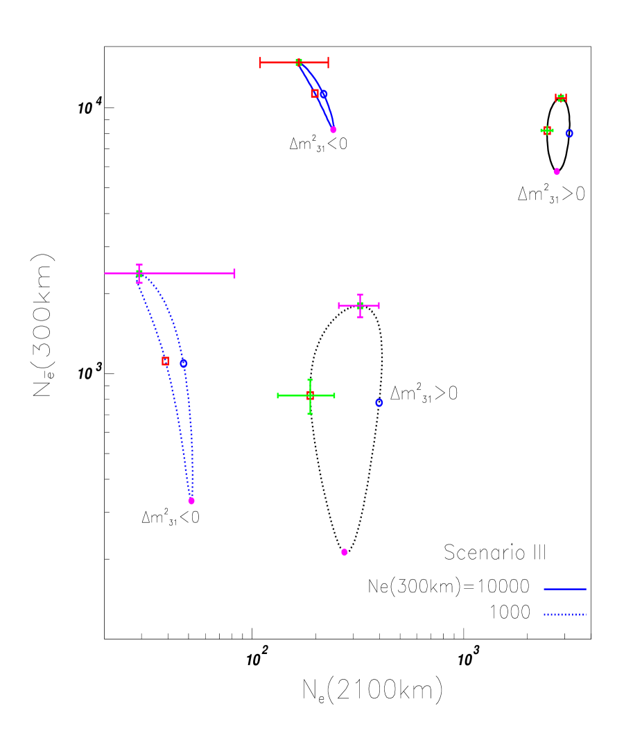
The situation of Scenario II can be improved if the statistics in $N_{e}(2100)$ are significantly increased. This can be achieved by using a larger detector and/or running for a longer period of time for the $N_{e}(2100)$ measurement. For Scenario III we set the detector size times the running time at $L$=2100 km to be 10 times larger than that of Scenario II, assuming that the number of events can be straightforwardly scaled up with the detector size. The running at 300 km is the same as in Scenario II. The resultant two-dimensional plot is shown Fig. 11. In this scenario, the sign of $\Delta m^{2}_{31}$ can be clearly determined at the 3$\sigma$ level, even for $N_{e}(300)$=1000 which corresponds to a very small $\sin^{2}(2\theta_{13})$ lying in the range ($0.006,0.01$), as indicated by the dotted curves in Fig. 11.

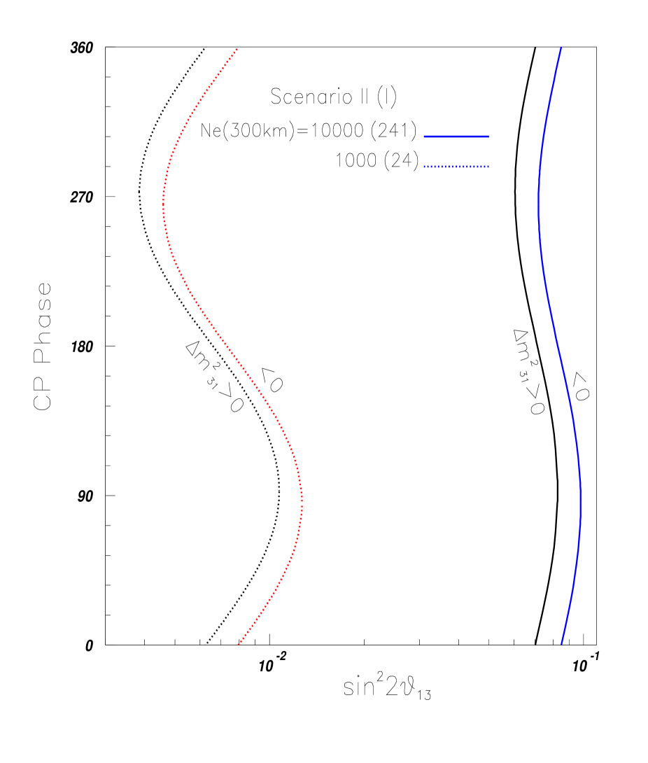
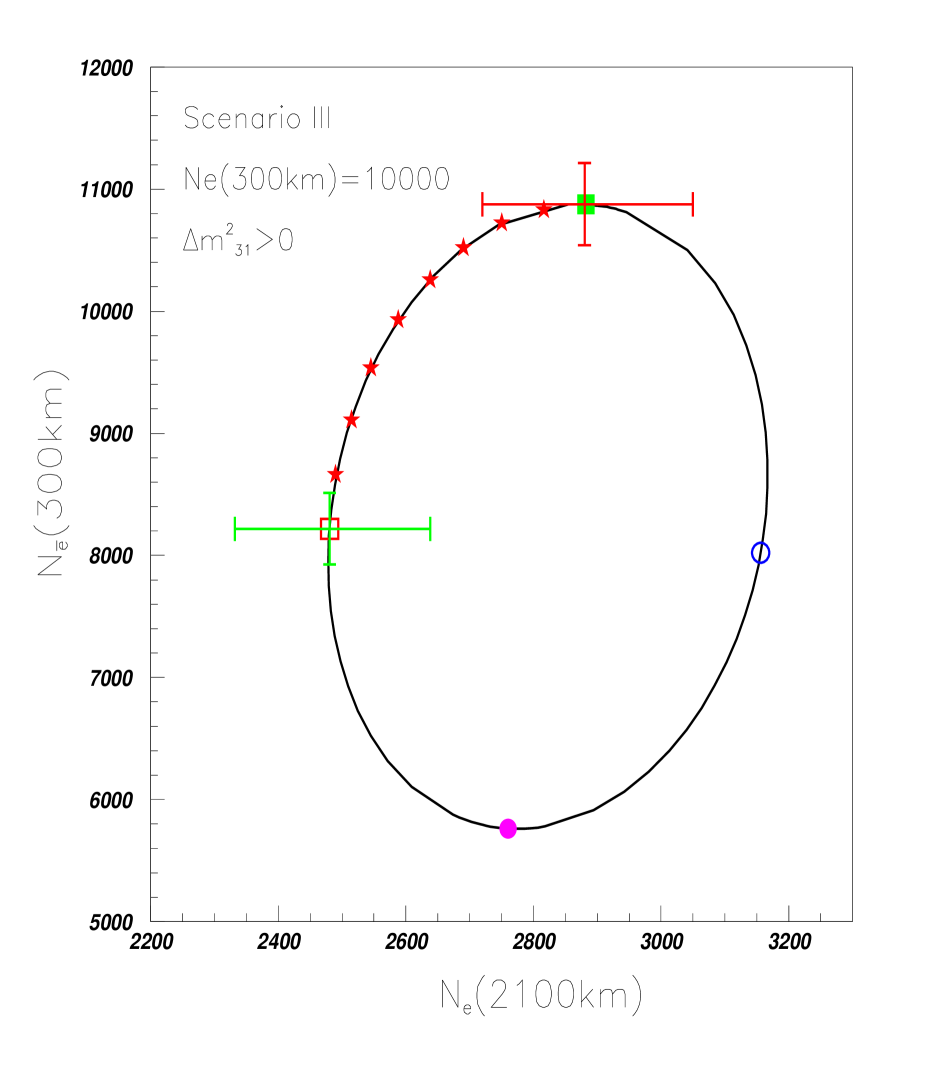
If $\Delta m^{2}_{31}$ is positive, a reasonably accurate determination of $\delta_{CP}$ can be made with no sgn($\Delta m^{2}_{31}$) or $\theta_{13}$ ambiguity, and the $\bar{\nu}_{\mu}$ beam is not needed at 2100 km even for very small $\sin^{2}(2\theta_{13})$ in the range ($0.006,0.01$). This is consistent with the results of Ref. [9], where it was found that a $\nu_{\mu}\to\nu_{e}$ and $\bar{\nu}_{\mu}\to\bar{\nu}_{e}$ measurement at short distance and a $\nu_{\mu}\to\nu_{e}$ measurement at a long distance could resolve parameter ambiguities for $\sin^{2}(2\theta_{13})>0.005$. To see the sensitivity more clearly for positive $\Delta m^{2}_{31}$, we replot the results in Figs. 12 and 13 respectively for $N_{e}(300)$=10000 and 1000. We see that for $N_{e}(300)=10000$, which corresponds to larger $\sin^{2}(2\theta_{13})$ ($0.06-0.1$) as shown in Fig. 3, the $CP$ phase can be determined better than 10^∘ at 3$\sigma$ for $\delta_{\rm CP}$ small or around 180^∘. The sensitivity deteriorates slowly when $\delta_{CP}$ moves away from $0^{\circ}$ or $180^{\circ}$, and the uncertainty becomes of the order of 25^∘ when $\delta_{\rm CP}$ is close to 90^∘ or 270^∘.

Even for $N_{e}(300)$=1000, which corresponds to very small $\sin^{2}(2\theta_{13})$ in the range of ($0.006,0.01$), the measurement of the $CP$ phase is still reasonably good. It is interesting to note that the sensitivity of the $CP$ measurement near $\delta_{\rm CP}$=0^∘ and 180^∘ for $N_{e}(300)=1000$ is comparable to that of the much higher number of events of $N_{e}(300)$=10000. Hence, in this scenario, either case can establish whether or not $CP$ in the lepton sector is violated if $\delta_{\rm CP}$ deviates by than 10^∘ from the $CP$ conserving points of $\delta_{\rm CP}$=0^∘ or 180^∘.

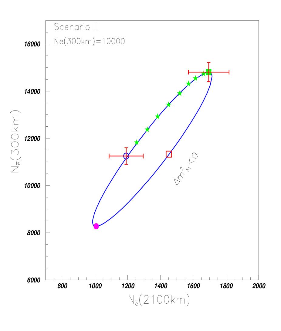
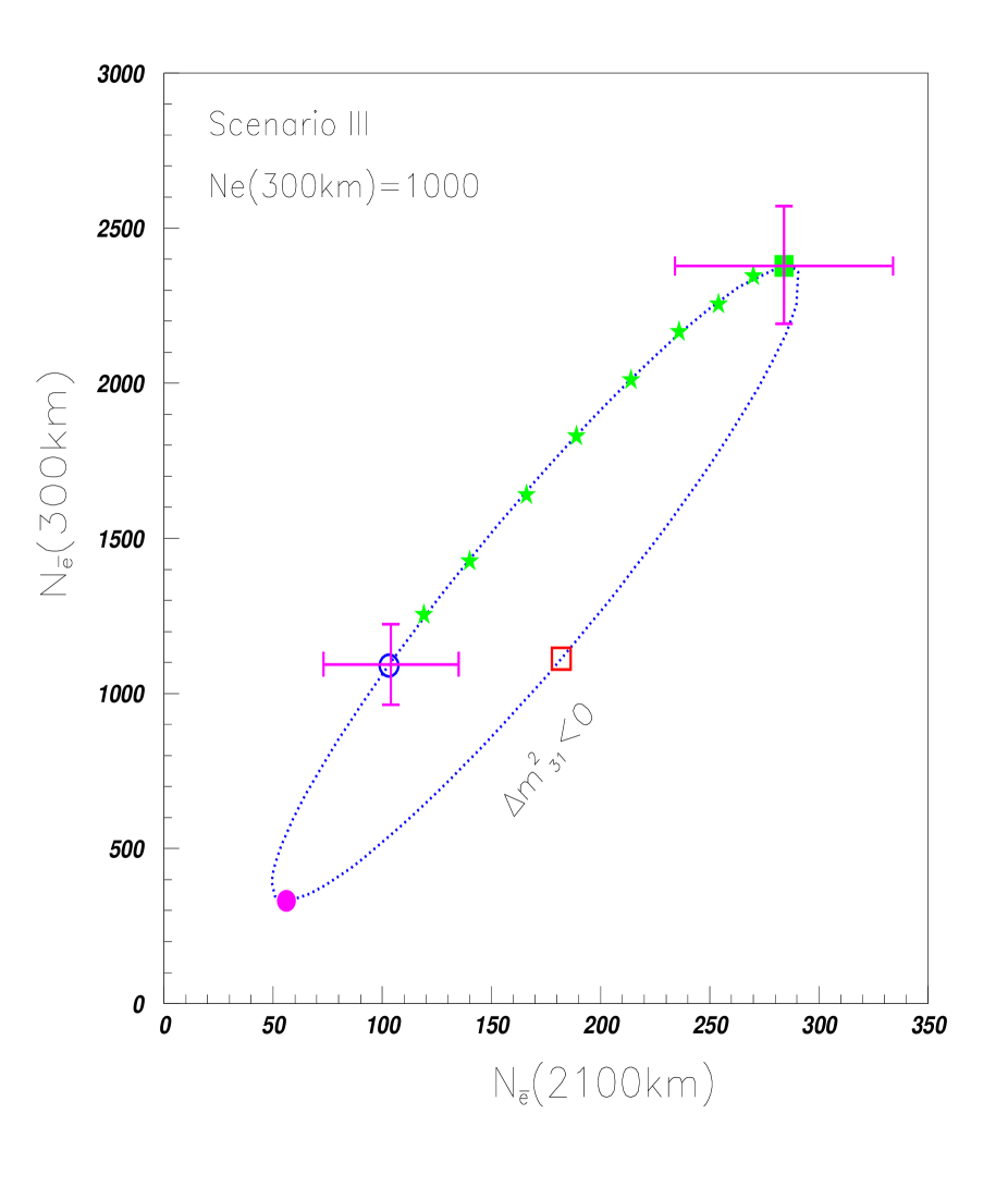
If $\Delta m^{2}_{31}$ is negative, the $\bar{\nu}_{\mu}\rightarrow\bar{\nu}_{e}$ oscillation is the favorable channel to investigate. Hence once it is clear that $\Delta{\rm m}^{2}_{31}$ is negative (see the next section for a detailed discussion), the $\bar{\nu}_{\mu}$ beam should be delivered to 2100 km to run for 5000 kt-yr. The results, which are the counterparts to Fig. 11, are shown in Fig. 14. With positron events at 2100 km the $CP$ phase can be well measured. To see the sensitivity more clearly, we replot the results in Figs. 15 and 16 for $N_{e}(300)$=10000 and 1000 respectively. The accuracy of the $\delta_{CP}$ measurement for $\Delta m^{2}_{31}<0$ using the $\bar{\nu}_{\mu}$ beam is about the same as that of the $\nu_{\mu}$ beam for $\Delta{\rm m}^{2}_{31}>0$, although the distinction between $\delta_{CP}$ in the range ($-\pi/2,\pi/2$) and $\delta_{CP}$ in the range ($\pi/2,3\pi/2$) is not as good for a $\bar{\nu}_{\mu}$ beam with $\Delta m^{2}_{31}<0$.

We have also done the analysis assuming a $\nu$ or $\bar{\nu}$ NBB of peak energy 5, 6, or 8 GeV is delivered to the detector at 2100 km. We found that for these cases the ellipses in Figs. 11 to 15 are much flatter than for the 4 GeV NBB, so that they do not do as well in resolving the degeneracy in $\delta_{CP}$.

IV Conclusion and discussion

We conclude that with a superbeam, such as that delivered by HIPA, the joint analysis at two baselines, of which one is an LBL at 300 km and the other a VLBL at 2100 km, can determine the $\Delta m^{2}_{31}$ sign and give a reasonably precise measurement of the $CP$ phase and $\theta_{13}$. To achieve this, both $\nu_{\mu}$ and $\bar{\nu}_{\mu}$ beams are needed for the LBL experiment. The survival events $\nu_{\mu}\rightarrow\nu_{\mu}$ and $\bar{\nu}_{\mu}\rightarrow\bar{\nu}_{\mu}$ are generally insensitive to the matter and $CP$ effects.

The initial HIPA $\nu_{\mu}$ beam with power 0.77 MW will run with exposure 22.5$\times$5 kt-yr at a detector at $L$=300 km to obtain both survival events $N_{\mu}(300)$ and appearance events $N_{e}(300)$. The former is used to improve the determination of the mixing angle $\theta_{23}$ and mass–squared difference $|\Delta m^{2}_{31}|$, so as to reduce the uncertainty of these crucial input parameters. The latter can show the existence of an appearance signal for $\sin^{2}(2\theta_{13})\geq 0.006$ and find a crude relation between $\delta_{CP}$ and $\theta_{13}$ as shown in Fig. 3.

A detailed determination of the oscillation parameters will require an upgrade of the HIPA beam power to 4 MW. Using our studies in this paper as a guide, we suggest as one possibility the following experimental steps using the upgraded HIPA beam:

Stage 1: Deliver a 4 MW $\nu$ 2^∘–OAB to a 450 kt detector at a distance of $L$=300 km for 2 years. The survival events $N_{\mu}(300)$ are used to determine more precisely the parameters $\theta_{23}$ and $|\Delta{m}^{2}_{31}|$. The appearance events $N_{e}(300)$ are used to refine the relation between $\delta_{CP}$ and $\theta_{13}$, as shown in Fig. 3.

Stage 2: A 4 MW $\nu$ NBB with peak energy around 4 GeV is delivered to a detector at $L$=2100 km, to run for 100$\times$5 kt-yr. The survival and appearance events $N_{\mu}(2100)$ and $N_{e}(2100)$ are used to determine the sign of $\Delta{m}^{2}_{31}$, with the most sensitivity coming from $N_{e}(2100)$ (see Fig. 4).

Stage 3: A 4 MW $\bar{\nu}_{\mu}$ 2^∘–OAB is delivered to the 300 km baseline detector for 450$\times$6 kt-yr and $N_{\bar{\mu}}(300)$ and $N_{\bar{e}}(300)$ are obtained. The data can only determine $\delta_{CP}$ and $\theta$ up to a 2-fold degeneracy because of the poor separation between $\delta$ and $\pi-\delta$ in the $N_{\bar{\mu}}(300)$ measurement, as demonstrated in Fig. 7.

Stage 4: A 4 MW $\nu_{\mu}$ ($\bar{\nu}_{\mu}$) NBB with peak energy around 4 GeV is delivered to the 2100 km baseline detector for 1000$\times$5 kt-yr if $\Delta{m}^{2}_{31}>0$ ($\Delta{m}^{2}_{31}<0$). Then at 3$\sigma$, the value of $\delta_{CP}$ can be determined to about $10^{\circ}$ for values close to $0^{\circ}$ or $180^{\circ}$, or to about $25^{\circ}$ for values close to $90^{\circ}$ or $270^{\circ}$. The distinction between $\delta_{CP}$ in the ranges $(-\pi/2,\pi/2)$ and $(\pi/2,3\pi/2)$ is better for $\Delta m^{2}_{31}>0$ than for $\Delta m^{2}_{31}<0$. The $\Delta{m}^{2}_{31}>0$ case is shown in Figs. 12 and 13 and that of $\Delta{m}^{2}_{31}<0$ in Figs. 15 and 16.

It is apparent from our calculation that in order to obtain enough statistics to provide a reasonably precise measurement of $\theta_{13}$ and $\delta_{CP}$ the total detector size and running time have to be sufficiently large. We have not attempted a detailed optimization; rather, we offer our calculation as an example for illustration. A search is still required to determine the optimal conditions for the measurement. Eventually uncertainties in the Earth matter density along a given baseline as well as uncertainties in the solar neutrino oscillation parameters $\theta_{12}$ and $\Delta m^{2}_{21}$ must also be taken into account.

REFERENCES

- [1] Y. Fukuda et al., Phys. Rev. Lett. B 81 (1998) 1562.
- [2] SNO collaboration, Phys. Rev. Lett. 87, 071301 (2001); arXiv:nucl-ex/0204008; nucl-ex/0204009.
- [3] HIPA: A multipurpose high intensity proton synchrotron at both 50 GeV and 3 GeV to be constructed at the Jaeri Tokai Campus, Japan has been approved in December, 2000 by the Japanese funding agency. The long baseline neutrino oscillation experiment is one of projects of the particle physics program of the facility. More about HIPA can be found at the website: ”http://jkj.tokai.jaeri.go.jp”.
- [4] J2K: Y. Ito, et. al., Letter of Intent: A Long Baseline Neutrino Oscillation Experiment the JHF 50 GeV Proton-Synchrotron and the Super-Kamiokande Detector, JHF Neutrino Working Group, Feb. 3, 2000; see also arXiv:hep-ex/0106019.
- [5] H. Chen, et al., Study Report: H2B, Prospect of a very Long Baseline Neutrino Oscillation Experiment, HIPA to Beijing, arXiv:hep-ph/0104266.
- [6] M. Aoki, K. Hagiwara, U. Hayato, T. Kobayashi, T. Nakaya, K. Nishikawa and N. Okamura, arXiv:hep-ph/0112338.
- [7] J. Burguet-Castell, M. B. Gavela, J. J. Gomez-Cadenas, P. Hernandez and O. Mena, Nucl. Phys. B 608, 301 (2001) [arXiv:hep-ph/0103258]; M. Freund, P. Huber and M. Lindner, Nucl. Phys. B 615, 331 (2001) [arXiv:hep-ph/0105071]; J. Pinney and O. Yasuda, Phys. Rev. D 64, 093008 (2001) [arXiv:hep-ph/0105087]; H. Minakata and H. Nunokawa, JHEP 0110, 001 (2001) [arXiv:hep-ph/0108085]; V. Barger, D. Marfatia and K. Whisnant, in Proc. of the APS/DPF/DPB Summer Study on the Future of Particle Physics (Snowmass 2001) ed. N. Graf, arXiv:hep-ph/0108090; Phys. Rev. D 65, 073023 (2002) [arXiv:hep-ph/0112119; T. Kajita, H. Minakata, and H. Nunokawa, arXiv:hep-ph/0112345; G. Barenboim, A. de Gouvea, M. Szleper, and M. Velasco, arXiv:hep-ph/0204208; A. Donini, D. Meloni and P. Magliozzi, arXiv:hep-ph/0206034.
- [8] P. Huber, M. Lindner, and W. Winter, arXiv:hep-ph/0204352.
- [9] V. Barger, D. Marfatia and K. Whisnant, Phys. Rev. D 66, 053007 (2002) [arXiv:hep-ph/0206038];
- [10] J. Burguet-Castell, M. B. Gavela, J. J. Gomez-Cadenas, P. Hernandez and O. Mena, arXiv:hep-ph/0207080.
- [11] Y. F. Wang, K. Whisnant, Z. Xiong, J. M. Yang and B.-L. Young, Phys. Rev. D65, 073021 (2002).
- [12] Y.F. Wang, K. Whisnant and Bing-Lin Young, Phys. Rev. D65, 073006 (2002).
- [13] S. Geer, Phys. Rev. D57, 6989 (1998).
- [14] L. Wolfenstein, Phys. Rev. D17, 2367 (1978); D20, 2634 (1979); V. Barger, K. Whisnant, S. Pakvasa and R.J.N. Phillips, Phys. Rev. D22, 2718 (1980); P. Langacker, J.P. Leveille and J. Sheiman, Phys. Rev. D27, 1228 (1983).
- [15] A. M. Dziewonski and D. L. Anderson, Phys. Earth Planet. Inter. 25, 297 (1981).
- [16] F. D. Stacey, Physics of the Earth (John Wiley & Sons, 1977); D. J. Anderson, Theory of the Earth (Blackwell Scientific Pub., 1989).
- [17] B.L.N. Kennet, et al., Georphys. J. Int., 122, 108 (1995); J.P. Montagner, et al., Geophys. J. Int., 125, 229 (1995).
- [18] Lian-You Shan, Bing-Lin Young and Xinmin Zhang, Phys. Rev. D66, 053012 (2002) [arXiv:hep-ph/0110414]; Lian-You Shan and Xinmin Zhang, Phys. Rev. D65, 113011 (2002); Lian-You Shan, Futian Liu, Yi-Fang Wang, Changgeng Yang, Bing-Lin Young and Xinmin Zhang, in preparation.
- [19] B. Jacobsson, T. Ohlsson, H. Snellman and W. Winter, Phys. Lett. 532, 259 (2002) [arXiv:hep-ph/0112138]; for a summary of different approaches to approximate the Earth’s density, see B. Jacobsson, T. Ohlsson, H. Snellman and W. Winter, talk given at NuFact ’02, London, 2002, arXiv:hep-ph/0209147.
- [20] T. Kobayashi, talk given at Fifth KEK Topical Conference, KEK,Japan, Nov. (2001).
- [21] The narrow band superbeam profiles are available at http://neutrino.kek.jp/JHF-VLBL.
- [22] The off-axis superbeam profiles are available at http://neutrino.kek.jp/ kobayasi/50gev/beam/.
- [23] Y.-F. Wang, arXiv:hep-ex/0010081, talk given at “NEW Initiatives in Lepton Flavor Violation and Neutrino Oscillations with Very Long Intense Muon Neutrino Sources”, Oct. 2-6, 2000, Hawaii, USA.
- [24] V. Barger, S. Geer, R. Raja and K. Whisnant, Phys. Rev. D 63, 113011 (2001).
- [25] Y. Itow et al., arXiv:hep-ex/0106019.
- [26] J. Busenitz, KamLAND collaboration, Intl. J. Mod. Phys. A 16 Suppl. B1, 742 (2001).
- [27] V. Barger, D. Marfatia and B. Wood, Phys. Lett. B498, 53 (2001).
- [28] M. Apollonio et al., Phys. Lett., B466, 415 (1999).