Higgs Boson Production at Hadron Colliders

Abstract

I report on a calculation of the inclusive Higgs boson production cross section at hadron colliders at next-to-next-to-leading order in QCD. The result is computed as an expansion about the threshold region. By continuing the expansion to very high order, we map the result onto basis functions and obtain the result in closed analytic form.

1 Introduction

At the LHC, gluon fusion will be the most important mechanism for Higgs boson production and discovery for masses below $\sim 700$ GeV. The discovery of the Higgs boson and the subsequent study of its properties therefore relies on a solid theoretical understanding of the gluon fusion production mechanism. Unfortunately, next-to-leading order (NLO) studies [1] of inclusive Higgs production do not provide this solid understanding. The NLO corrections are so large (of order $70-100$%) that one cannot assume that they provide a reliable estimate of the total cross section. The unsettled nature of such an important signal clearly calls for a renewed effort to bring this process under control.

Earlier this year, we computed the full NNLO corrections to the hadronic cross section for Higgs boson production [2] as an expansion about the threshold region. The expansion was carried out to very high ($18$th!) order so that any uncertainty due to uncalculated higher terms would be very small. Very recently, this calculation has been confirmed by an exact NNLO calculation of the partonic cross section [3]. Shortly before this conference began, we extended our calculation of the expansion to sufficiently high order as to allow us to invert the series and obtain the exact result for the hadronic cross section. In addition, we have used the same methods to compute the NNLO corrections to pseudo-scalar Higgs production, for which we present preliminary results [4].

2 The Calculation

In the limit that all quark masses except that of the top quark vanish, gluons couple to Higgs only via top quark loops. This coupling can be approximated by an effective Lagrangian [5] corresponding to the limit $m_{t}\to\infty$, which is valid for a large range of $M_{H}$, including the currently favored region between 100 and 200 GeV. The effective Lagrangian is

$${\cal L}_{\rm eff}=-\frac{H}{4v}C_{1}(\alpha_{s})\,G_{\mu\nu}^{a}G^{a\,\mu\nu}\,,$$ (1)

where $G_{\mu\nu}^{a}$ is the gluon field strength tensor, $H$ is the Higgs field, $v\approx 246$ GeV is the vacuum expectation value of the Higgs field and $C_{1}(\alpha_{s})$ is the Wilson coefficient, which for this calculation we need to order $(\alpha_{s}^{3})$ [6].

For the pseudo-scalar Higgs, we again assume that gluon fusion through top-quark loops is the dominant production mechanism. This assumption is not valid in all models, especially when the ratio of vacuum expectation values is large. The effective Lagrangian for pseudo-scalar production is [7]

$$\begin{split}&{\cal L}_{Agg}=-g_{t}\,\frac{A}{v}\left[\tilde{C}_{1}\,\tilde{\cal O}_{1}+\tilde{C}_{2}\,\tilde{\cal O}_{2}\right]\,,\\ &\tilde{\cal O}_{1}=G^{a}_{\mu\nu}\tilde{G}^{a,\mu\nu}\,,\quad\tilde{\cal O}_{2}=\partial_{\mu}\left(\sum_{q}\bar{q}\gamma^{\mu}\,\gamma_{5}q\right)\,.\end{split}$$ (2)

where $A$ is the pseudo-scalar Higgs field, $g_{t}$ is a model-dependent coupling constant and $\tilde{G}^{a}_{\mu\nu}$ is the dual of the field strength tensor:

$$\begin{split}\tilde{G}^{a}_{\mu\nu}=\epsilon_{\mu\nu\alpha\beta}\,G^{a,\alpha\beta}\,.\end{split}$$ (3)

The calculation breaks down into four contributions: virtual corrections to two loops, single-real-emission to one loop, double-real-emission at tree-level and mass factorization. The virtual, single-real and mass factorization terms are computed exactly in closed analytic form. The double-real contribution is by far the hardest part of the calculation because of the complicated phase space integrals. We have computed this contribution by expanding the phase space integration about the threshold limit, where the partonic center-of-mass energy is close to the Higgs mass ($M_{H}^{2}/\hat{s}\equiv x\to 1$). Because Higgs production is dominated by threshold corrections, the series expansion converges quite rapidly. So, we compute double-real-emission, and thus the partonic cross section, as an expansion in $(1-x)$ and $\ln(1-x)$. Note that if all coefficients are computed, this is an exact expression. In fact, one can obtain the exact result for the partonic cross section from a finite number of terms.

3 Inverting the series

If one were to know the basis functions that make up the exact result and one could expand the series out to enough terms, one could invert the series, mapping it onto the basis functions. One can obtain a reasonable ansatz for the basis functions by examining the result for Drell-Yan production [8]. Using polylogagrithm identities [9] this result can be expressed in terms of functions which are analytic in $(1-x)$ and powers of $\ln(1-x)$ times functions which are analytic in $(1-x)$. Each of these basis functions can be multiplied by a pre-factor. Again using the Drell-Yan result as a guide and knowledge of the gluon splitting function, one can make an ansatz of the possible pre-factors. The ansätze for pre-factors and basis functions are shown in Table 1.

Table 1: Ansatz pre-factors and functions for exact result

$\displaystyle{1}$	$\displaystyle{1}$	$\displaystyle{\ln(x)}$
$\displaystyle{\frac{1}{x}}$	$\displaystyle{\ln^{2}(x)}$	$\displaystyle{\ln^{3}(x)}$
$\displaystyle{\frac{1}{1-x}}$	$\displaystyle{{\mathop{\rm Li}_{2}\nolimits}(1-x)}$	$\displaystyle{{\mathop{\rm Li}_{2}\nolimits}(1-x)\ln(x)}$
$\displaystyle{\frac{1}{1+x}}$	$\displaystyle{{\mathop{\rm Li}_{2}\nolimits}(1-x^{2})}$	$\displaystyle{{\mathop{\rm Li}_{2}\nolimits}(1-x^{2})\ln(x)}$
$\displaystyle{1-x}$	$\displaystyle{{\mathop{\rm Li}_{3}\nolimits}(1-x)}$	$\displaystyle{{\mathop{\rm Li}_{3}\nolimits}\left(-\frac{1-x}{x}\right)}$
$\displaystyle{(1-x)^{2}}$	$\displaystyle{{\mathop{\rm Li}_{3}\nolimits}(1-x^{2})}$	$\displaystyle{{\mathop{\rm Li}_{3}\nolimits}\left(-\frac{1-x^{2}}{x^{2}}\right)}$
$\displaystyle{(1-x)^{3}}$	$\displaystyle{{\mathop{\rm Li}_{3}\nolimits}\left(\frac{1-x}{1+x}\right)}$	$\displaystyle{{\mathop{\rm Li}_{3}\nolimits}\left(-\frac{1-x}{1+x}\right)}$

One sees that there are $7$ pre-factors and $14$ functions meaning that if one can expand the series result out to $98$ terms, one can map the result onto these $98$ functions. The mapping can be verified by computing still higher terms and comparing to the expansion of the mapped functions. To carry out this program, we have computed the double-real radiation terms out to order $(1-x)^{100}$. Since the series starts at order $(1-x)^{-1}$, this gives us $102$ terms.

It turns out that the $1/x$ pre-factor never occurs in the cross section (in Ref. [8] it appears in the Drell-Yan correction term, not the Drell-Yan cross section) and the last two basis functions, ${\mathop{\rm Li}_{3}\nolimits}((1-x)/(1+x))$ and ${\mathop{\rm Li}_{3}\nolimits}(-(1-x)/(1+x))$ always occur together as the difference. Thus, after the fact, we see that $78$ terms would have sufficed to determine the functional form. The additional $24$ terms significantly over-determine the system and provide a strong verification of the result. In addition, we have compared our result with that recently reported in Ref. [3] using a completely independent method, and find exact agreement.

4 Hadronic Results

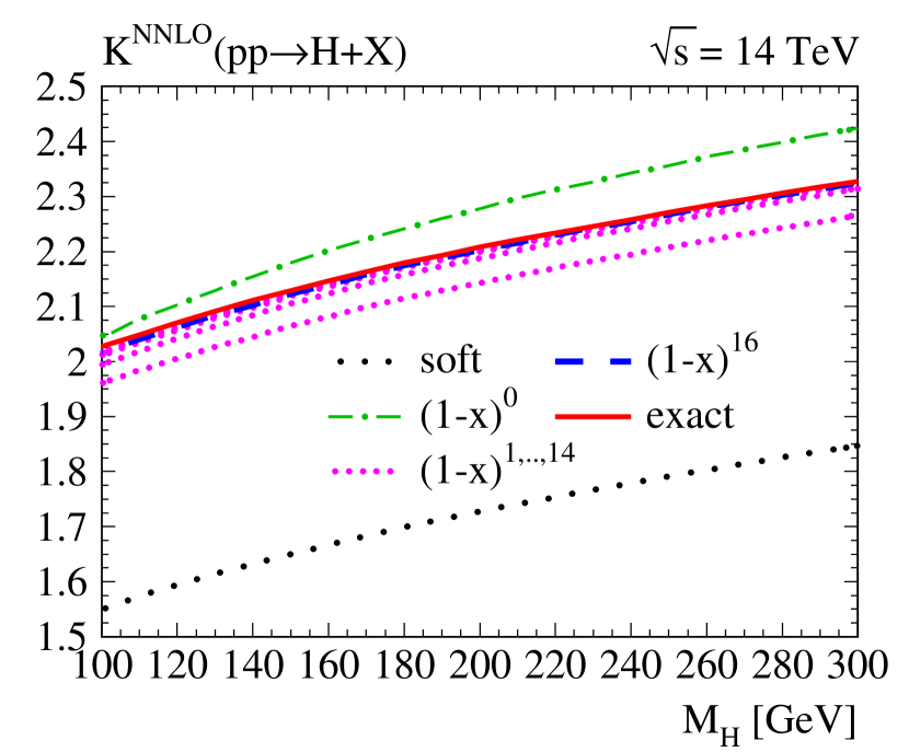
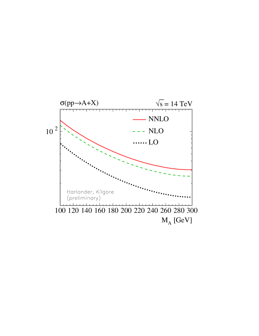
In Ref. [2], the partonic cross section was computed using a series expansion out to order $(1-x)^{16}$. The difference between using that series expansion and the exact calculation is quite small (less than $\sim 1\%$) as one would expect. In light of the intrinsic uncertainty due to scale dependence of order $\pm 10\%$, this difference is completely negligible. The convergence of the series for scalar Higgs production is shown in Fig. 1. Preliminary results for pseudo-scalar Higgs production is shown in Fig. 2

Figure 1: NNLO cross section for Higgs production using the exact partonic cross section and series expansions truncated at the indicated values.

Figure 2: Cross section for pseudo-scalar Higgs production at leading order (LO), NLO and NNLO (preliminary) [4]. The model dependent couling $g_{t}$ has been set to unity.

We obtain our hadronic results by folding the partonic cross section with appropriate parton distribution functions (PDFs). We use approximate NNLO parton distribution functions [10] based on an approximation of the evolution equation [11, 12].