CP Violation Effects on $B^{0}_{s,d}\rightarrow\it l^{+}\it l^{-}$ in Supersymmetry
at Large $\tan\beta$

Tarek Ibrahim^a,b and Pran Nath^b

a. Department of Physics, Faculty of Science, University of Alexandria,
Alexandria, Egypt
b. Department of Physics, Northeastern University, Boston, MA 02115-5000, USA

  Abstract

An analytic analysis of the CP violating effects arising from the soft SUSY breaking parameters on the decays $B^{0}_{s,d}\rightarrow\it l^{+}\it l^{-}$ at large $\tan\beta$ is given. It is found that the phases have a strong effect on the branching ratio and in some regions of the parameter space they can lead to a variation of the branching ratio by as much as 1-2 orders of magnitude. These results have important implications for the discovery of the $B^{0}_{s}\rightarrow\mu^{+}\mu^{-}$ signal in RUNII of the Tevatron and further on how the parameter space of SUSY models will be limited once the signal is found.

1 Introduction

Recently there has been a great amount of interest in the rare process $B^{0}_{s}\rightarrow\mu^{+}\mu^{-}$[1, 2, 3] as it offers an opportunity to probe physics beyond the standard model[1, 2, 3, 4, 5, 6, 7]. Thus in the standard model the branching ratio is rather small[2], i.e., $B(\bar{B}^{0}_{s}\rightarrow\mu^{+}\mu^{-})$ $=$$(3.1\pm 1.4)\times 10^{-9}$ (for $|V_{ts}|=0.04\pm 0.002$) while in supersymmetric models it can get three orders of magnitude larger for large $\tan\beta$ and the branching ratio can be as large as $10^{-6}$. This result is very exciting in view of the fact that the sensitivity of the Tevatron to this decay will improve by two orders of magnitude allowing a test of a class of supersymmetric models even before any sparticles are found. Thus while the current limit on this decay is $B(\bar{B}^{0}_{s}\rightarrow\mu^{+}\mu^{-})$ $<$$(2.6)\times 10^{-6}$ it is estimated that the RUNII of the Tevatron could be sensitive to a branching ratio down to the level of $10^{-8}$ or even lower[5]. While this sensitivity is still too small to test the standard model prediction, it is large enough to explore significant portions of the parameter space of supersymmetric models such as mSUGRA[8]. The previous analyses have mostly been in the context of CP conservation except for the works of Refs.[9, 10]. In Ref.[9] effects of CP violation on lepton asymmetries, ie., $(l^{+}l^{+}-l^{-}l^{-})/(l^{+}l^{+}+l^{-}l^{-})$ in decays of $B\bar{B}$ pairs were studied, while in Ref.[10] CP asymmetry in B and $\bar{B}$ decays was investigated but only a cursory mention of the effect of CP violation on the size of the branching ratio, which is primarily the quantity which will be measured at the Tevatron, was made in Ref.[10]. The effects of CP phases on the Higgs sector were ignored in these works. However, it is known that at large $\tan\beta$ CP mixing effects in the neutral Higgs sector are very significant and cannot be ignored[11, 12]. In this analysis we give a complete analysis of the effects of CP violation on the decay $B^{0}_{d,s}\rightarrow\it l^{+}\it l^{-}$ valid at large $\tan\beta$ including the effects of CP violation in the neutral Higgs sector which mediates the decay. The focus of our work is the effect of CP violation on the branching ratio $B(\bar{B}^{0}_{d,s}\rightarrow\it l^{+}\it l^{-})$. Specifically we would like to see the size of the variation in the branching ratio when the phases are included in the analysis and to see if such variations will allow the branching ratio to lie within reach of RUNII of the Tevatron.

In supersymmetric models CP phases arise naturally via the soft breaking masses. Thus the mSUGRA model allowing for complex soft parameters contains two phases and the parameter space of such models can be characterized by $m_{0},m_{\frac{1}{2}},|A_{0}|,\tan\beta,\theta_{\mu},\alpha_{A}$ where $m_{0}$ is the universal scalar mass, $m_{\frac{1}{2}}$ is the universal gaugino mass, $|A_{0}|$ is the universal trilinear coupling, $\tan\beta=<H_{2}>/<H_{1}>$ where $H_{2}$ gives mass to the up quark and $H_{1}$ gives mass to the down quark and the leptons, $\theta_{\mu}$ is the phase of the Higgs mixing parameter $\mu$ and $\alpha_{A}$ is the phase of the trilinear couplings $A_{0}$. In extended SUGRA models with nonuniversalities and in the minimal supersymmetric standard model (MSSM) one can have many more phases. Specifically the $U(1),SU(2),SU(3)$ gaugino masses $m_{i}$ (i=1,2,3) can have phases so that $m_{i}=|m_{i}|e^{i\xi_{i}}$ and such phases play an important role in SUSY phenomena at low energy. An important constraint on models with CP violation is that of the experimental limits on the electron and on the neutron electric dipole moments (edms)($d_{e}<4.3\times 10^{-27}ecm$[13], $d_{n}<6.5\times 10^{-26}~{}ecm$[14]). These constraints can be satisfied in a variety of ways[15, 16, 17, 18, 19]. The limit on the edm of $H_{g}^{199}$ is also known to a high degree of accuracy ($d_{H_{g}}<9\times 10^{-28}ecm$[20]) and recent analyses have also included this constraint[21]. Specifically in scenarios with the cancellation mechanism[18] and in scenario with phases only in the third generation[19] one can accommodate large CP violating phases and their inclusion can affect supersymmetric phenomena in a very significant way. In this work we will focus on the contribution from the so called counter term diagram (Fig.1) which gives an amplitude proportional to $\tan^{3}\beta$ for large $\tan\beta$. The decay $B^{0}_{d^{\prime}}\rightarrow\it l^{+}\it l^{-}$ ($d^{\prime}=d,s$) is governed by the effective Hamiltonian[2]

$$H_{eff}=-\frac{G_{F}e^{2}}{4\sqrt{2}\pi^{2}}V_{tb}V_{td^{\prime}}^{*}(C_{S}O_{S}+C_{P}O_{P}+C_{S}^{\prime}O_{S}^{\prime}$$

$$+C_{P}^{\prime}O_{P}^{\prime}++C_{10}O_{10})_{Q}$$ (1)

where

$$O_{S}=m_{b}(\bar{d}^{\prime}_{\alpha}P_{R}b_{\alpha})(\bar{l}l),~{}~{}O_{P}=m_{b}(\bar{d}^{\prime}_{\alpha}P_{R}b_{\alpha})(\bar{l}\gamma_{5}l),$$

$$O_{S}^{\prime}=m_{d^{\prime}}(\bar{d}^{\prime}_{\alpha}P_{L}b_{\alpha})(\bar{l}l),O_{P}^{\prime}=m_{d^{\prime}}(\bar{d}^{\prime}_{\alpha}P_{L}b_{\alpha})(\bar{l}\gamma_{5}l),$$

$$O_{10}=(\bar{d}^{\prime}_{\alpha}\gamma^{\mu}P_{L}b_{\alpha})(\bar{l}\gamma_{\mu}\gamma_{5}l)$$ (2)

and where the subscript $Q$ in Eq.(1) is the scale where the quantities are being evaluated. The branching ratio $B(B^{0}_{d^{\prime}}\rightarrow\it l^{+}\it l^{-})$ is given by

$$B(\bar{B}^{0}_{d^{\prime}}\rightarrow\it l^{+}\it l^{-})=\frac{G_{F}^{2}\alpha^{2}M_{B_{d^{\prime}}}^{5}\tau_{B_{d^{\prime}}}}{16\pi^{3}}|V_{tb}V_{td^{\prime}}^{*}|^{2}$$

$$(1-\frac{4m_{\it l}^{2}}{M^{2}_{B_{d^{\prime}}}})^{1/2}\{(1-\frac{4m_{\it l}^{2}}{M^{2}_{B_{d^{\prime}}}})|f_{S}|^{2}+|f_{P}+2m_{\it l}f_{A}|^{2}\}$$ (3)

where $f_{i}$ (i=S,P) and $f_{A}$ are defined as follows

$$f_{i}=-\frac{i}{2}f_{B_{d^{\prime}}}(\frac{C_{i}m_{b}-C_{i}^{\prime}m_{d^{\prime}}}{m_{d^{\prime}}+m_{b}}),f_{A}=-\frac{if_{B_{d^{\prime}}}}{2M_{B_{d^{\prime}}}^{2}}C_{10}$$ (4)

Additionally in the above one should include the SUSY QCD correction[22] which behaves like $\mu\tan\beta$ and can produce a significant effect in the large $\tan\beta$ region.

Figure 1: The counter term diagram. which contributes to the branching ratio $B^{0}_{s}\rightarrow\it l^{+}\it l^{-}$ and produces the leading term in the amplitude proportional to $\tan^{3}\beta$.

2 Effects of CP Violation on $B_{s}^{0}\rightarrow\mu^{+}\mu^{-}$

We discuss now the effects of CP violation on the decay $B_{s}^{0}\rightarrow\mu^{+}\mu^{-}$. As pointed out above the diagram which gives the largest contribution in the large $\tan\beta$ region is the counter term diagram and involves the exchange of Higgs poles. In the absence of CP violation the Higgs sector diagonalizes into a CP even and a CP odd sector. However, it is well known that loop effects induce a CP violation in the Higgs sector and generate a mixing of CP even and CP odd sectors[11, 12]. As a consequence CP effects will enter Fig.1 not only in the vertices involving charginos and squarks but also in the Higgs poles and the vertices involving the Higgs. CP violation in the Higgs sector can be exhibited by parameterizing the Higgs VEVs in the presence of CP violating phases as follows:

$$(H_{1})=(H_{1}^{0},H_{1}^{-})=(v_{1}+\phi_{1}+i\psi_{1},H_{1}^{-})/\sqrt{2},$$

$$(H_{2})=(H_{2}^{+},H_{2}^{0})=e^{i\theta_{H}}(H_{2}^{+},v_{2}+\phi_{2}+i\psi_{2})/\sqrt{2})$$ (5)

where in general $\theta_{H}$ is non-vanishing as a consequence of the minimization conditions of the Higgs potential. In the presence of CP violating phases the CP even and the CP odd sectors of the Higgs fields mix and thus the Higgs matrix is a $4\times 4$ matrix in the basis $\phi_{1},\phi_{2},\psi_{1},\psi_{2}$. In the basis $\phi_{1},\phi_{2},\psi_{1D},\psi_{2D}$ where

$$\psi_{1D}=\sin\beta\psi_{1}+\cos\beta\psi_{2},$$

$$\psi_{2D}=-\cos\beta\psi_{1}+\sin\beta\psi_{2}$$ (6)

the $\psi_{2D}$ field decouples and is identified as the Goldstone and one is left with a remaining $3\times 3$ $(mass)^{2}$ matrix which mixes CP even and CP odd states. The Higgs mass matrix can be diagonalized by the transformation

$$RM^{2}_{Higgs}R^{T}=diag(M_{H_{1}}^{2},M_{H_{2}}^{2},M_{H_{3}}^{2})$$ (7)

where the eigen values $(m_{H_{1}},m_{H_{2}},m_{H_{3}})$ are now admixtures of CP even and CP odd states and we arrange the eigenvalues so that in the limit of no CP violation one has the identification $(m_{H_{1}},m_{H_{2}},m_{H_{3}})$$\rightarrow$ $(m_{H},m_{h},m_{A})$ where (h, H) are the (light, heavy) CP even Higgs bosons and A is the CP odd Higgs boson. The diagonalization modifies the vertices which connect the Higgs with the quarks and the leptons. One finds that the interaction Lagrangian for the Higgs vertices that enter in the counter term diagram is now given by

$$L_{ffH}=-(gm_{b}/2m_{W}cos\beta)\Sigma_{j=1}^{3}\bar{b}[R_{j1}-i\gamma_{5}sin\beta R_{j3}]bH_{j}$$

$$-(gm_{l}/2m_{W}cos\beta)\Sigma_{j=1}^{3}\bar{l}[R_{j1}-i\gamma_{5}sin\beta R_{j3}]lH_{j}$$ (8)

In the SUSY sector we carry out the analysis in the scenario with minimal flavor violation where the squark mass matrices are assumed flavor-diagonal. Under this assumption we find

$$C_{S}=-\frac{m_{\it l}}{\sqrt{2}m_{W}^{2}\cos^{3}\beta}\sum_{j=1}^{3}\sum_{s=1}^{2}m_{\chi_{s}^{+}}\frac{R_{j1}^{2}}{M_{H_{j}}^{2}}\psi_{s}$$ (9)

$$C_{P}=\frac{m_{\it l}\tan^{2}\beta}{\sqrt{2}m_{W}^{2}\cos\beta}\sum_{j=1}^{3}\sum_{s=1}^{2}m_{\chi_{s}^{+}}\frac{R_{j3}^{2}}{M_{H_{j}}^{2}}\psi_{s}$$ (10)

$$\psi_{s}=\sum_{q=t,c,u}U_{s2}\lambda_{qq}\{(\frac{m_{W}V_{s1}}{2\sin^{2}\theta_{W}})[\cos^{2}{\frac{\theta_{q}}{2}}f_{3}({m^{2}_{\tilde{q}_{1}}}/{m_{\chi_{s}^{+2}}})$$

$$+\sin^{2}{\frac{\theta_{q}}{2}}f_{3}({m^{2}_{\tilde{q}_{2}}}/{m_{\chi_{s}^{+2}}})]+\frac{m_{q}V_{s2}\sin\theta_{q}}{4\sqrt{2}\sin^{2}\theta_{W}\sin\beta}e^{i\phi_{q}}\Delta f_{3}\}$$ (11)

where $\Delta f_{3}$= $f_{3}({m^{2}_{\tilde{q}_{2}}}/{m_{\chi_{s}^{+2}}})$- $f_{3}({m^{2}_{\tilde{q}_{1}}}/{m_{\chi_{s}^{+2}}})$, $\tilde{q}_{1}(\tilde{q}_{2})$ is the heavier (lighter) squark and $\theta_{q}$ and $\phi_{q}$ are defined by

$$\sin\theta_{q}=\frac{2m_{q}|A_{q}m_{0}-\mu^{*}\cot\beta|}{m_{\tilde{q}_{1}}^{2}-m_{\tilde{q}_{2}}^{2}}$$ (12)

$$\sin\phi_{q}=\frac{m_{0}|A_{q}|\sin\alpha_{A_{q}}+|\mu|\sin\theta_{\mu}\cot\beta}{|m_{0}A_{q}-\mu^{*}\cot\beta|}$$ (13)

In Eq.(11) $U$ and $V$ are the diagonalizing matrices for the chargino mass matrix $M_{C}$ so that $U^{*}M_{C}V^{-1}=diag(m_{\chi_{1}^{\pm}},m_{\chi_{2}^{\pm}})$ and finally $f_{3}$ in Eq.(11) is a form factor defined by $f_{3}(x)={x}lnx/(1-x)$. For the diagram of Fig.1 $C_{S}^{\prime}$ and $C_{P}^{\prime}$ are defined as follows

$$C_{S}^{\prime}(counter)=(C_{S}(counter)[\lambda_{qq}\rightarrow\lambda_{qq}^{*}])^{*}$$

$$C_{P}^{\prime}(counter)=-(C_{P}(counter)[\lambda_{qq}\rightarrow\lambda_{qq}^{*}])^{*}$$ (14)

where $\lambda_{qq}=(V_{qb}V_{qd^{\prime}}^{*}/V_{tb}V_{td^{\prime}}^{*})_{CKM}$ and the subscript means that the matrix V here is the CKM matrix. Eqs.(9-13) give the most general result for the minimal flavor violation with inclusion of phases without any approximations. Neglecting the squark mixings for the first two generations Eq.(11) simplifies so that

$$\psi_{s}=U_{s2}\{(\frac{m_{W}V_{s1}}{2\sin^{2}\theta_{W}})[\lambda_{uu}f_{3}(y_{\tilde{u}_{1s}})+\lambda_{cc}f_{3}(y_{\tilde{c}_{1s}})$$

$$+\cos^{2}{\frac{\theta_{t}}{2}}f_{3}(y_{\tilde{t}_{1s}})+\sin^{2}{\frac{\theta_{t}}{2}}f_{3}(y_{\tilde{t}_{2s}})]$$

$$+\frac{m_{t}V_{s2}\sin\theta_{t}}{4\sqrt{2}\sin^{2}\theta_{W}\sin\beta}e^{i\phi_{t}}[f_{3}(y_{\tilde{t}_{2s}})-f_{3}(y_{\tilde{t}_{1s}})]\}$$ (15)

where $y_{\tilde{u}_{1s}}$ etc are defined by $y_{\tilde{u}_{1s}}=({m^{2}_{\tilde{u}_{1}}}/{m_{\chi_{s}^{+2}}})$, $y_{\tilde{c}_{1s}}=({m^{2}_{\tilde{c}_{1}}}/{m_{\chi_{s}^{+2}}})$, $y_{\tilde{t}_{1s}}={m^{2}_{\tilde{t}_{1}}}/{m_{\chi_{s}^{+2}}}$, $y_{\tilde{t}_{2s}}={m^{2}_{\tilde{t}_{2}}}/{m_{\chi_{s}^{+2}}}$.

3 Numerical Size of CP Effects

Eqs.(9)-(15) constitute the new results of this analysis as they include the effects of CP violation. In the limit when we neglect the CP phases our approximation Eq.(15) agrees with the result of Bobeth etal.[2] at large $\tan\beta$. The phases can increase or decrease the branching ratio. We focus on the region of the parameter space where an enhancement occurs and this region is of considerable relevance for the detection of the $B^{0}_{s}\rightarrow\mu^{+}\mu^{-}$ signal.

Figure 2: The ratio of the branching ratios $B(B^{0}_{s}\rightarrow\mu^{+}\mu^{-})/B(B^{0}_{s}\rightarrow\mu^{+}\mu^{-})_{0}$, where $B(B^{0}_{s}\rightarrow\mu^{+}\mu^{-})_{0}$ is the branching ratio when all phases are set to zero, as a function of the CP violating phase $\alpha_{A}$ for values of $|A_{0}|$ of 1,2,3,4,5 in the ascending order of the curves. The other parameters are $m_{0}=200$ GeV, $m_{1/2}=200$ GeV, $\tan\beta=50$, $\xi_{1}=\xi_{2}=\pi/4$, $\xi_{3}=0$, and $\theta_{\mu}=2$.

Figure 3: Exhibition of the branching ratio $B^{0}_{s}\rightarrow\mu^{+}\mu^{-}$ as a function of $\tan\beta$. The three top curves correspond in descending order to cases (a), (b) and (c) of Table 1 where the input parameters for each case is recorded (all masses in GeV and all angles in radians). The lower solid, dashed and dot-dashed curves have the same inputs as the top solid, dashed and dot-dashed curves except that all phases are set to zero. The edms corresponding to the top three curves for the case $\tan\beta=50$ are given in Table1.

Figure 4: Same as Fig.3 except that the lower three curves have all phases set to $\pi$.

Table 1. Electron, neutron and $H_{g}$ edms
case	$m_{0}$, $m_{\frac{1}{2}}$, $|A_{0}|$	$\alpha_{A}$, $\xi_{1}$, $\xi_{2}$, $\xi_{3}$	$d_{e}$	$d_{n}$	$d_{H_{g}}$
(a)	$200,200,4$	$1,.5,.659,.633$	$1.45\times 10^{-27}$	$9.2\times 10^{-27}$	$7.2\times 10^{-27}$
(b)	$370,370,4$	$2,.6,.653,.672$	$-1.14\times 10^{-27}$	$-7.9\times 10^{-27}$	$2.87\times 10^{-26}$
(c)	$320,320,3$	$.8,.4,.668,.6$	$-3.5\times 10^{-27}$	$7.1\times 10^{-27}$	$2.9\times 10^{-26}$

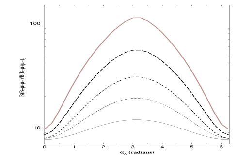
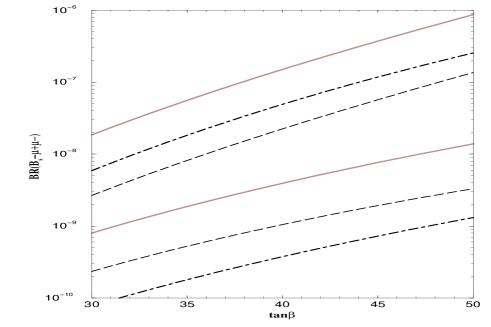
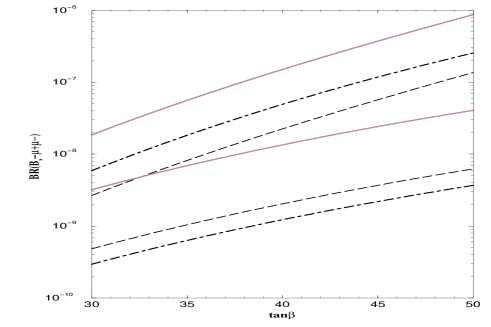
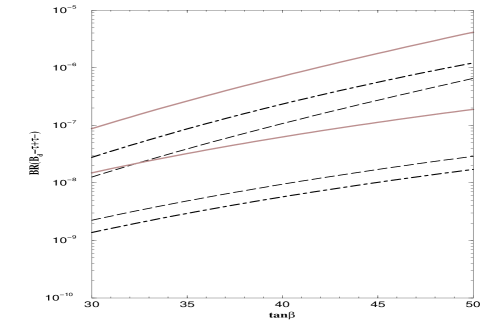
In Fig.2 we give a plot of the ratio $B(B^{0}_{s}\rightarrow\mu+\mu^{-})/B(B^{0}_{s}\rightarrow\mu+\mu^{-})_{0}$, where $B(B^{0}_{s}\rightarrow\mu+\mu^{-})_{0}$ is the branching ratio in the absence of phases, as a function of the phase $\alpha_{A}$ of the trilinear coupling $A_{0}$ for values of $|A_{0}|$ ranging from 1 to 5. In each case we find that the ratio of branching ratios shows a strong dependence on $\alpha_{A}$. Specifically for the case $|A_{0}|=5$ the ratio can become as large as $10^{2}$. Thus Fig.(2) shows that with phases the branching ratio can be significantly modified. There are many contributing factors to this phenomenon. Thus in Eqs.(9),(10) and (15) we find several quantities that depend on the phases. These include the chargino masses, the Higgs masses, the mixings $R_{j1}$ and $R_{j3}$ etc. However, the largeness of the effect arises mostly from the variation in $\psi_{s}$. Here one finds that in some regions of the parameter space the masses of the stops and their mixings are strongly affected by the CP phases which affect $\sin\theta_{t}$ and $f_{3}$ and their combined effect can generate a large enhancement of the amplitude when the phases are included. In Fig.3 we exhibit the branching ratio $B^{0}_{s}\rightarrow\mu^{+}\mu^{-}$ as a function of $\tan\beta$ for various values of the phases and compare the results to the CP conserving case where the phases are all set to zero. The analysis of Fig.4 is identical to that of Fig.3 except that a comparison is made with the CP conserving case where the phases are all set to $\pi$. One finds that often points in the parameter space which would otherwise (i.e., when phases all vanish or are equal to $\pi$) lie below the sensitivity of $\sim 10^{-8}$ for the branching ratio, which is what the RUNII of the Tevatron can achieve in the future, can now be moved into the region of sensitivity of the Tevatron.

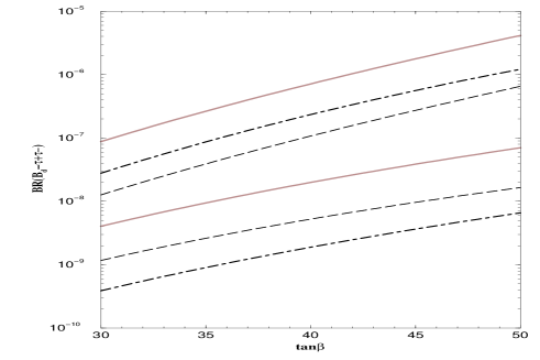
We have checked that using the cancellation mechanism there exist regions of the parameter space where the experimental constraints on the edms of the electron, of the neutron, and of $H_{g}^{199}$ are satisfied. For $H_{g}^{199}$ the atomic edm constraint can be translated into a contrainst on a specific combination of the chromo electric dipole moment of u, d and s quarks, so that $C_{H_{g}}=|d_{d}^{C}-d_{u}^{C}-0.012d_{s}^{C}|$ is contrained to satisfy $C_{H_{g}}<3.0\times 10^{-26}cm$. An example is given in Table1. As shown in Ref.[23] one uses scaling to generate a trajectory where cancellations occur and the edm constraints are satisfied starting from a given cancellation point. We have checked that this is the case for the region such as in Table1. In Fig.5 we exhibit the effect of CP phases on the branching ratio of $B^{0}_{d}\rightarrow\tau^{+}\tau^{-}$ and compare the result to the CP conserving cases where all the phases are set to zero. (An analysis without phases for this process is also given in Ref.[7]). The analysis of Fig.6 is identical to that of Fig.6 except that a comparison with CP conserving cases is made by setting all the phases to $\pi$. It would be interesting to see if some of the region of Figs. 5 and 6 would be accessible to experiment in the future. An interesting study has recently appeared correlating the $B^{0}_{d,s}-\bar{B}^{0}_{d,s}$ mass difference $\Delta M_{d,s}$ with $B^{0}_{d,s}\rightarrow\mu^{+}\mu^{-}$ in supersymmetry for large $\tan\beta$[24]. It would be interesting to investigate this correlation in the presence of phases in MSSM. However, this requires an analysis of the $B^{0}_{d,s}-\bar{B}^{0}_{d,s}$ mass difference with inclusion of phases in the supersymmetric loop contribution to the $\Delta M_{d,s}$. This possibility is under investigation.

4 Conclusion

In conclusion in this work we have derived analytic results for the effects of CP violating phases on the branching ratio $B^{0}_{d^{\prime}}\rightarrow\it l^{+}\it l^{-}$ arising from the chargino-stop exchange contribution in the counter term diagram in the large $\tan\beta$ region. It is found that the branching ratio in general is sensitive to the CP phases and that the branching ratio can vary in some parts of the parameter space by up to 1-2 orders of magnitude. These results have important implications for the search for this signal and for the interpretation of it in limiting the SUSY parameter space once the signal is found. Of course significant effects of order 50-100% can be obtained with significantly smaller phases than those in Table 1 and here the edm constraints can be satisfied over a much larger parameter space. In the above analysis we have not included the effects of the gluino and the neutralino exchanges. Inclusion of these will bring in a strong dependence on additional phases $\xi_{1}$ and $\xi_{3}$. A full analysis of the CP violating effects valid also for small $\tan\beta$ will be discussed elsewhere.

Figure 5: Exhibition of the branching ratio $B^{0}_{d}\rightarrow\tau^{+}\tau^{-}$ as a function of $\tan\beta$. The three top curves correspond in descending order to cases (a), (b) and (c) of Table 1 where the input parameters for each case is recorded (all masses in GeV and all angles in radians). The lower solid, dashed and dot-dashed curves have the same inputs as the top solid, dashed and dot-dashed curves except that all phases are set to zero. The edms corresponding to the top three curves for the case $\tan\beta=50$ are given in Table1.

Figure 6: Same as Fig.5 except that the lower three curves have all phases set equal to $\pi$.

ACKNOWLEDGEMENTS

This research was supported in part by NSF grant PHY-0139967.

References

- [1] S. R. Choudhury and N. Gaur, Phys. Lett. B 451, 86 (1999); K. S. Babu and C. Kolda, Phys. Rev. Lett. 84, 228 (2000).
- [2] C. Bobeth, T. Ewerth, F. Kruger and J. Urban, Phys. Rev. D 64, 074014 (2001) [arXiv:hep-ph/0104284].
- [3] P. H. Chankowski and L. Slawianowska, Acta Phys. Polon. B 32 (2001) 1895 ; H.E. Logan and U. Nierste, Nucl. Phys. B586, 39(2000) ; G. Isidori and A. Retico, JHEP 0111, 001 (2001) ; C. S. Huang, W. Liao, Q. S. Yan and S. H. Zhu, Phys. Rev. D 63, 114021 (2001) [Erratum-ibid. D 64, 059902 (2001)] ; Phys. Rev. D 63 (2001) 11402; (E) D64 (2001) 059902; ; A. J. Buras, P. H. Chankowski, J. Rosiek and L. Slawianowska, arXiv:hep-ph/0207241; Z. Xiong and J. M. Yang, Nucl. Phys. B 628, 193 (2002) [arXiv:hep-ph/0105260].
- [4] A. Dedes, H. K. Dreiner, U. Nierste, and P. Richardson, Phys. Rev. Lett. 87, 251804 (2001); A. Dedes, H. K. Dreiner and U. Nierste, arXiv:hep-ph/0207026;
- [5] R. Arnowitt, B. Dutta, T. Kamon and M. Tanaka, Phys. Lett. B 538 (2002) 121.
- [6] S. Baek, P. Ko, and W. Y. Song, arXiv:hep-ph/0206008; arXiv:hep-ph/0208112
- [7] J.K. Mizukoshi, X. Tata and Y. Wang, hep-ph/0208078
- [8] A.H. Chamseddine, R. Arnowitt and P. Nath, Phys. Rev. Lett. 49, 970 (1982); R. Barbieri, S. Ferrara and C.A. Savoy, Phys. Lett. B 119, 343 (1982); L. Hall, J. Lykken, and S. Weinberg, Phys. Rev. D 27, 2359 (1983): P. Nath, R. Arnowitt and A.H. Chamseddine, Nucl. Phys. B 227, 121 (1983). For reviews, see P. Nath, R. Arnowitt and A.H. Chamseddine, ”Applied N=1 Supergravity”, world scientific, 1984; H.P. Nilles, Phys. Rep. 110, 1(1984).
- [9] L. Randall and S. f. Su, Nucl. Phys. B 540, 37 (1999).
- [10] C. S. Huang and W. Liao, Phys. Lett. B 538, 301 (2002); Phys. Lett. B 525, 107 (2002); C. S. Huang, hep-ph/0210314.
- [11] A. Pilaftsis, Phys. Rev. D58, 096010; Phys. Lett.B435, 88(1998); A. Pilaftsis and C.E.M. Wagner, Nucl. Phys. B553, 3(1999); D.A. Demir, Phys. Rev. D60, 055006(1999); S. Y. Choi, M. Drees and J. S. Lee, Phys. Lett. B 481, 57 (2000); M. Boz, Mod. Phys. Lett. A 17, 215 (2002); ; M. Carena, J. R. Ellis, A. Pilaftsis and C. E. Wagner, Nucl. Phys. B 625, 345 (2002).
- [12] T. Ibrahim and P. Nath, Phys.Rev.D63:035009,2001; ibid, arXiv:hep-ph/0204092; T. Ibrahim, Phys.Rev.D64, 035009(2001); S. W. Ham, S. K. Oh, E. J. Yoo, C. M. Kim and D. Son, arXiv:hep-ph/0205244.
- [13] E. Commins, et. al., Phys. Rev. A50, 2960(1994).
- [14] P.G. Harris et.al., Phys. Rev. Lett. 82, 904(1999).
- [15] See, e.g., J. Ellis, S. Ferrara and D.V. Nanopoulos, Phys. Lett. B114, 231(1982); M. Dugan, B. Grinstein and L. Hall, Nucl. Phys. B255, 413(1985); R.Garisto and J. Wells, Phys. Rev. D55, 611(1997).
- [16] P. Nath, Phys. Rev. Lett.66, 2565(1991); Y. Kizukuri and N. Oshimo, Phys.Rev.D46,3025(1992).
- [17] K.S. Babu, B. Dutta and R. N. Mohapatra, Phys. Rev. D61, 091701(2000).
- [18] T. Ibrahim and P. Nath, Phys. Lett. B 418, 98 (1998); Phys. Rev. D58, 111301(1998); T. Falk and K Olive, Phys. Lett. B 439, 71(1998); M. Brhlik, G.J. Good, and G.L. Kane, Phys. Rev. D59, 115004 (1999); A. Bartl, T. Gajdosik, W. Porod, P. Stockinger, and H. Stremnitzer, Phys. Rev. 60, 073003(1999); S. Pokorski, J. Rosiek and C.A. Savoy, Nucl.Phys. B570, 81(2000); E. Accomando, R. Arnowitt and B. Dutta, Phys. Rev. D 61, 115003 (2000); U. Chattopadhyay, T. Ibrahim, D.P. Roy, Phys.Rev.D64:013004,2001; C. S. Huang and W. Liao, Phys. Rev. D 61, 116002 (2000). For analyses in the context string and brane models see, M. Brhlik, L. Everett, G. Kane and J. Lykken, Phys. Rev. Lett. 83, 2124, 1999; Phys. Rev. D62, 035005(2000); E. Accomando, R. Arnowitt and B. Datta, Phys. Rev. D61, 075010(2000); T. Ibrahim and P. Nath, Phys. Rev. D61, 093004(2000).
- [19] D. Chang, W-Y.Keung,and A. Pilaftsis, Phys. Rev. Lett. 82, 900(1999).
- [20] S. K. Lamoreaux et.al., Phys. Rev. Lett. 57, 3125 (1986).
- [21] T. Falk, K.A. Olive, M. Prospelov, and R. Roiban, Nucl. Phys. B560, 3(1999); V. D. Barger, T. Falk, T. Han, J. Jiang, T. Li and T. Plehn, Phys. Rev. D 64, 056007 (2001); S.Abel, S. Khalil, O.Lebedev, Phys. Rev. Lett. 86, 5850(2001)
- [22] M. Carena, D. Garcia, U. Nierste and C. E. Wagner, Nucl. Phys. B 577, 88 (2000)
- [23] T. Ibrahim and P. Nath, Phys. Rev. D 61, 093004 (2000)
- [24] A. J. Buras, P. H. Chankowski, J. Rosiek and L. Slawianowska, arXiv:hep-ph/0210145.