SLAC-PUB-9373 hep-ph/0208115 Pseudoscalar Higgs boson production at hadron colliders in NNLO QCD

Abstract

We compute the total cross-section for direct production of the pseudoscalar Higgs boson in hadron collisions at next-to-next-to-leading order (NNLO) in perturbative QCD. The ${\cal O}(\alpha_{s}^{2})$ QCD corrections increase the NLO production cross-section by approximately $20-30$ per cent.

I Introduction

Supersymmetry is one of the most popular extensions of the Standard Model (SM). Generically, supersymmetric theories predict a very rich spectrum of elementary particles. In particular, the Higgs boson sector of the Minimal Supersymetric Standard Model (MSSM) consists of two complex Higgs doublets. After electroweak symmetry breaking, three Higgs fields are absorbed by the $W^{\pm}$ and $Z$ bosons into their longitudinal degrees of freedom; the remaining five degrees of freedom are physical Higgs bosons. In addition to the standard Higgs boson $(h)$, a heavier neutral Higgs boson $(H)$, two charged scalar Higgs bosons $(H^{\pm})$, and a neutral pseudoscalar Higgs boson $(A)$ appear in the spectrum.

The tree-level masses of the Higgs bosons in the MSSM are usually described in terms of two independent parameters: the mass of the pseudoscalar Higgs boson $m_{A}$ and the ratio of the vacuum expectation values of the two Higgs doublets $\tan\beta=v_{1}/v_{2}$. Currently, these parameters are restricted by the experiments at LEP which set a lower bound $m_{A}>91.9~{}{\rm GeV}$ and exclude the values $0.5<\tan\beta<2.4$ lep ; lepwg . Future searches for the pseudoscalar Higgs boson will be carried out at the Tevatron and at the LHC. It is therefore important to obtain a reliable theoretical estimate of its production cross-section in hadron collisions.

The pseudoscalar Higgs boson does not couple to the gauge bosons at tree level; the major mechanisms for producing it are the gluon-gluon fusion mechanism $gg\to A$ and the associated production process $gg,qq\to Aqq$. The relative significance of the production channels depends on the mass of the Higgs boson and the value of $\tan\beta$. For larger values of $\tan\beta$, the coupling of the pseudoscalar Higgs boson to up quarks, $g_{\rm up}\sim m_{u}/\tan\beta$, decreases while the coupling of the Higgs boson to down quarks, $g_{\rm down}\sim m_{d}\tan\beta$, increases. As a consequence, the phenomenology of the axial Higgs for large values of $\tan\beta$ is very different from the phenomenology of the SM Higgs boson. For the $(t,b)$ family, the Higgs boson interaction with bottom quarks dominates for values of $\tan\beta\geq 10$.

Gluon-gluon fusion through a quark triangle-loop is the dominant production channel of the light pseudoscalar Higgs boson in hadron collisions; there is no squark-loop contribution to the $ggA$ coupling. In this Letter we study the gluon-gluon fusion cross-section for small and moderate values of $\tan\beta$. We can then neglect the contribution of bottom quarks and focus on the production of the pseudoscalar Higgs boson through the top-quark loop. In addition, we consider small values of the pseudoscalar Higgs boson mass, $m_{A}\leq 300~{}{\rm GeV}$. Since $m_{A}\ll 2m_{t}$, where $m_{t}$ is the mass of the top-quark, the interaction of the pseudoscalar Higgs boson with gluons and light quarks can be described by the effective Lagrangian Chetyrkin:1998mw

$${\cal L}=\frac{A}{v\tan\beta}\left[\tilde{C}_{1}~{}G_{\mu\nu}\tilde{G}^{\mu\nu}+\tilde{C}_{2}\partial_{\mu}J_{5}^{\mu}\right],$$ (1)

where $G_{\mu\nu}$ is the color field-strength tensor and

$$\tilde{G}_{\mu\nu}=\epsilon_{\mu\nu\alpha\beta}~{}G^{\alpha\beta},~{}~{}~{}J_{5}^{\mu}=\sum\limits_{i}^{n_{f}}\bar{q}_{i}\gamma_{\mu}\gamma_{5}q_{i}.$$

The Wilson coefficients $\tilde{C}_{1}$ and $\tilde{C}_{2}$ are given by

$$\tilde{C}_{1}=-\frac{\alpha_{s}(\mu)}{16\pi},$$

$$\tilde{C}_{2}=\left(\frac{\alpha_{s}(\mu)}{\pi}\right)^{2}\left(\frac{1}{8}-\frac{1}{4}L_{t}\right),$$ (2)

where $\alpha_{s}(\mu)$ is the $\overline{\rm MS}$ coupling constant, $n_{f}$ is the number of massless quark flavors and $L_{t}=\log(\mu^{2}/m_{t}^{2})$.

The renormalization in higher orders of the perturbation theory of the effective Lagrangian in Eq. (1) is subtle. Because of the axial anomaly, the derivative of the axial current of light quarks, $\partial_{\mu}J_{5}^{\mu}$, mixes under renormalization with the operator $G_{\mu\nu}~{}\tilde{G}^{\mu\nu}$. The renormalization procedure must preserve the anomaly relation

$$\partial_{\mu}J_{5}^{\mu}=\frac{\alpha_{s}(\mu)n_{f}}{8\pi}~{}G_{\mu\nu}\tilde{G}^{\mu\nu}.$$ (3)

A detailed discussion of the effective Lagrangian and its renormalization can be found in Ref. Chetyrkin:1998mw .

The Levi-Civita tensor $\epsilon_{\mu\nu\alpha\beta}$ and the $\gamma_{5}$ Dirac matrix are four-dimensional and their treatment in dimensional regularization is a delicate problem. For calculational convenience we use the approach suggested in Ref. Larin:tq . According to this prescription the $\gamma_{5}$ matrix is represented as $\gamma_{5}=i/24~{}\epsilon_{\mu\nu\alpha\beta}\gamma^{\mu}\gamma^{\nu}\gamma^{\alpha}\gamma^{\beta}$ and the axial-vector current as $J_{5}^{\mu}=1/2\bar{\psi}(\gamma_{\mu}\gamma_{5}-\gamma_{5}\gamma_{\mu})\psi$. With this substitution we can factor out the product of two Levi-Civita tensors from the production cross-section and evaluate it in terms of $d=4-2\epsilon$ dimensional metric tensors $\delta_{\mu\nu}$, using

$$\epsilon_{\mu_{1}\mu_{2}\mu_{3}\mu_{4}}\epsilon^{\nu_{1}\nu_{2}\nu_{3}\nu_{4}}=-\left|\begin{array}[]{cccc}\delta_{\mu_{1}}^{\nu_{1}}&\delta_{\mu_{1}}^{\nu_{2}}&\delta_{\mu_{1}}^{\nu_{3}}&\delta_{\mu_{1}}^{\nu_{4}}\\ \delta_{\mu_{2}}^{\nu_{1}}&\delta_{\mu_{2}}^{\nu_{2}}&\delta_{\mu_{2}}^{\nu_{3}}&\delta_{\mu_{2}}^{\nu_{4}}\\ \delta_{\mu_{3}}^{\nu_{1}}&\delta_{\mu_{3}}^{\nu_{2}}&\delta_{\mu_{3}}^{\nu_{3}}&\delta_{\mu_{3}}^{\nu_{4}}\\ \delta_{\mu_{4}}^{\nu_{1}}&\delta_{\mu_{4}}^{\nu_{2}}&\delta_{\mu_{4}}^{\nu_{3}}&\delta_{\mu_{4}}^{\nu_{4}}\\ \end{array}\right|.$$ (4)

We have checked that the above prescription is consistent with the renormalization procedure of Ref. Chetyrkin:1998mw by calculating the decay rate of the pseudoscalar Higgs boson through NNLO. Our results are in agreement with the expressions for the decay rate given in Ref. Chetyrkin:1998mw , where a four-dimensional treatment of the Levi-Civita tensors was employed.

In this Letter we present the NNLO QCD corrections to the pseudoscalar Higgs boson production cross-section in hadron collisions. Various partonic processes contribute to the cross-section at this order. Specifically, we have to compute: a) virtual corrections to $gg\to A$, $q\bar{q}\to A$ up to ${\cal O}(\alpha_{s}^{2})$; b) virtual corrections to single real emission processes $gg\to Ag$, $qg\to Aq$, $\bar{q}g\to A\bar{q}$, $q\bar{q}\to Ag$, up to ${\cal O}(\alpha_{s})$; and c) double real emission processes $gg\to Agg$, $gg\to Aq\bar{q}$, $qg\to Aqg$, $q\bar{q}\to Agg$, $q\bar{q}\to Aq\bar{q}$. We evaluate the above corrections using the method introduced in Ref. babis for the algorithmic evaluation of phase-space integrals.

II Partonic Cross-Sections

In this section we present analytic expressions for the partonic cross-sections $i+j\to A+X$, where $i,j=q,\bar{q},g$. We write

$$\hat{\sigma}_{ij}=\sigma_{0}^{(A)}\left[\phi_{ij}^{(0)}+\left(\frac{\alpha_{s}}{\pi}\right)\phi_{ij}^{(1)}+\left(\frac{\alpha_{s}}{\pi}\right)^{2}\phi_{ij}^{(2)}\right],$$ (5)

where

$$\sigma_{0}^{(A)}=\frac{\pi}{256v^{2}\tan^{2}\beta}\left(\frac{\alpha_{s}}{\pi}\right)^{2}.$$ (6)

The coefficients $\phi^{(k)}_{ij}$ are very similar to the coefficients $\eta^{(k)}_{ij}$ of the perturbative expansion of the partonic cross-sections for the production of the scalar Higgs boson babis . We can then write

$$\phi^{(k)}_{ij}\equiv\delta\phi^{(k)}_{ij}+\eta^{(k)}_{ij}.$$ (7)

For convenience, we present here the difference $\delta\phi^{(k)}_{ij}=\phi^{(k)}_{ij}-\eta^{(k)}_{ij}$. The $\eta^{(k)}_{ij}$ terms are listed in Section IV of Ref. babis .

We set the renormalization and the factorization scales equal to the mass of the Higgs boson $m_{A}$. At LO we find

$$\delta\phi^{(0)}_{ij}=0.$$ (8)

At NLO we obtain

$$\delta\phi^{(1)}_{gg}=\frac{1}{2}\delta(1-x),$$ (9)

and

$$\delta\phi^{(1)}_{qg,q\bar{q}}=0.$$ (10)

The NLO terms are in agreement with the results of Ref. spira .

At NNLO the differences $\delta\phi^{(2)}_{ij}$ are very simple. For both $\phi^{(2)}_{ij}$ and $\eta^{(2)}_{ij}$ we find the same polylogarithmic terms; the differences contain simple logarithms and the Riemann $\zeta_{2}$ constant. We obtain

$$\delta\phi^{(2)}_{gg} = \left[\left(\frac{{\it L_{t}}}{3}-\frac{21}{16}\right)\delta\left(1-x\right)+\frac{2}{3}x\ln^{2}\left(x\right)+x\ln\left(x\right)\right.$$ (11)

$$\left.-\frac{1}{6}\left(10x-1\right)\left(x-1\right)\right]{\it n_{f}}+6{\left[\frac{\ln(1-x)}{(1-x)}\right]_{+}}$$

$$+\left(3\zeta_{2}+\frac{1939}{144}-\frac{19}{8}{\it L_{t}}\right)\delta\left(1-x\right)$$

$$-6x\left({x}^{2}-x+2\right)\ln\left(1-x\right)-9x\ln^{2}\left(x\right)$$

$$+\frac{3}{2}\left(2{x}^{4}-4{x}^{3}+13{x}^{2}+x-10\right){\frac{\ln\left(x\right)}{(x-1)}}$$

$$+\frac{1}{4}\left(x-1\right)\left(11{x}^{2}+35x-154\right),$$

$$\delta\phi^{(2)}_{qg} = \frac{2}{3}\left(-2x+2+{x}^{2}\right)\ln\left(1-x\right)-{\frac{28}{9}}x\ln^{2}\left(x\right)$$ (12)

$$+\left[{\frac{22}{3}}+10x-\frac{{x}^{2}}{3}\right]\ln\left(x\right)+{\frac{17}{6}}{x}^{2}-{\frac{191}{9}}x$$

$$+{\frac{337}{18}},$$

$$\delta\phi^{(2)}_{q\bar{q}} = \left[-{\frac{32}{27}}x\ln\left(x\right)+{\frac{16}{27}}\left(x^{2}-1\right)\right]{\it n_{f}}$$ (13)

$$+{\frac{32}{27}}x\ln^{2}\left(x\right)+{\frac{32}{27}}{\left(3+8x\right)\ln\left(x\right)}$$

$$-\frac{16}{27}\left(x-1\right)\left({x}^{2}+10x+11\right),$$

$$\delta\phi^{(2)}_{qq^{\prime}} = -{\frac{16}{9}}x\ln^{2}\left(x\right)+\left[\frac{16}{3}x+{\frac{32}{9}}\right]\ln\left(x\right)$$ (14)

$$+{\frac{8}{9}}\left(x-1\right)\left(x-11\right),$$

and

$$\delta\phi^{(2)}_{qq} = -{\frac{64}{27}}x\ln^{2}\left(x\right)+\left[{\frac{32}{9}}+{\frac{176}{27}}x\right]\ln\left(x\right)$$ (15)

$$+{\frac{8}{27}}\left(x-1\right)\left(3x-37\right).$$

The above results are valid if the renormalization and factorization scales are equal to the mass of the Higgs boson, $\mu_{f}=\mu_{r}=m_{A}$. The complete functional dependence of the partonic cross-sections on these scales can be easily restored by solving the DGLAP equation and the renormalization group equation and using the above expressions as the boundary conditions. This procedure is outlined in Ref. babis .

III Numerical Results

Figure 1: The pseudoscalar Higgs boson production cross-section at the LHC at leading (dotted), next-to-leading (dashed-dotted) and next-to-next-to-leading (solid) order. The two curves for each case correspond to $\mu_{r}=\mu_{f}=m_{A}/2$ (upper) and $\mu_{r}=\mu_{f}=2m_{A}$ (lower).

We now discuss the numerical impact of the NNLO corrections on the pseudoscalar Higgs boson production cross-section at the LHC and the Tevatron. To calculate the cross-section we must convolute the hard scattering partonic cross-sections of Section II with the appropriate parton distribution functions, according to the factorization formula

$$\sigma_{A}=x\sum\limits_{ij}\left[\bar{f}_{i}^{(h_{1})}\otimes\bar{f}_{j}^{(h_{2})}\otimes(\sigma_{ij}(z)/z)\right](x).$$ (16)

Here $\bar{f}_{i}^{(h)}$ is the $\overline{\rm MS}$ distribution function of the parton $i$ in the hadron $h$, $\otimes$ denotes the standard convolution,

$$(f\otimes g)(x)\equiv\int_{0}^{1}dydzf(y)g(z)\delta(x-yz),$$ (17)

and $x=m_{A}^{2}/s$, where $s$ is the square of the total center of mass energy of the hadron-hadron collision.

The complete NNLO parton distribution functions are not yet available. In Ref. msrt an approximate NNLO evolution neervenvogt has been implemented in order to determine the NNLO MRST parton distribution functions. We use these approximate solutions for the numerical evaluation of the pseudoscalar Higgs boson production cross-section keeping the same initialization parameters as in Ref. babis .

To demonstrate the convergence properties of the perturbative series for the hadronic cross-section, we present the LO, NLO and NNLO results for both the LHC and the Tevatron. In order to improve upon the heavy-top quark approximation, we normalize our results to the leading-order cross-section with the exact dependence on $m_{t}$.

The total cross-section for the LHC is shown in Fig. 1.

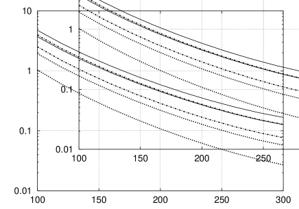
Figure 2: The pseudoscalar Higgs boson production cross-section at the Tevatron at leading (solid), next-to-leading (dashed) and next-to-next-to-leading (dotted) order. The two curves for each case correspond to $\mu_{r}=\mu_{f}=m_{A}/2$ (upper) and $\mu_{r}=\mu_{f}=2m_{A}$ (lower).

From Fig.1 we observe that the scale dependence of the Higgs production cross-section at NNLO is approximately $15\%$; this is a factor of two smaller than the NLO scale dependence and a factor of four less than the scale variation at LO. Despite the scale stabilization, the corrections are rather large; the NLO corrections increase the LO cross-section by about $70\%$, and the NNLO corrections further increase it by approximately $30\%$. The $K$ factor, defined as the ratio of the NNLO cross-section and the LO cross-section, is approximately two. In Fig.2 we plot the values of the Higgs production cross-section at the Tevatron. The NNLO $K$ factor is approximately three, and the residual scale dependence is approximately $30\%$. The $K$ factors for the production of the pseudoscalar Higgs boson and the scalar Higgs boson hkhard ; babis are comparable in magnitude; this is a consequence of the similarity of the corresponding partonic cross-sections as discussed in Section II.

Figure 3: The pseudoscalar Higgs boson production cross-section at the LHC at leading (dotted), next-to-leading (dashed) and next-to-next-to-leading (solid) order as the function of factorization and renormalization scale $\mu$. The mass of the Higgs boson is $115~{}{\rm GeV}$.

In Ref. babis we have argued that since the dominant contribution to the integrated cross-section for the scalar Higgs boson comes from the region close to the Higgs boson production threshold, we should choose values of the scale $\mu$ which are smaller than the mass of the Higgs boson. This choice decreases the NNLO corrections and the Higgs boson production cross-section increases as compared to conventional choice of the scales, $\mu_{r}=\mu_{f}=m_{H}$. The production cross-section for the pseudoscalar Higgs boson exhibits the same behavior. In Fig. 3 we show an example, where we plot the production cross-section for $m_{A}=115~{}{\rm GeV}$. We equate the renormalization and factorization scales and vary the factorization scale from $\mu=25~{}{\rm GeV}$ up to the mass of the pseudoscalar Higgs boson. The plot illustrates that for smaller values of $\mu$, the NLO cross-section increases more rapidly than the NNLO cross-section, and the difference between the NLO and the NNLO results becomes smaller. Therefore, the convergence of the perturbative series is improved for smaller values of the factorization scale.

IV Conclusions

In this Letter we presented the NNLO QCD corrections for the production cross-section of the pseudoscalar Higgs boson in hadron collisions. Our results are valid in the heavy top-quark limit and for small to moderate values of $\tan\beta$.

The analytic expressions which we presented here and those for the scalar Higgs boson babis are very similar. In both cases, the QCD corrections are large and important for quantitative estimates of the hadronic cross-sections at the Tevatron and the LHC. The size of the NNLO corrections for the pseudoscalar Higgs boson indicates that the perturbative expansion of the production cross-section converges, albeit slowly. A similar convergence behavior was observed for the SM Higgs boson hadronic production cross-section hkhard ; babis .

In order to verify the compatibility of the prescription of Ref. Larin:tq for the Levi-Civita tensor with the Wilson coefficients for the effective Lagrangian in Eq. (1), derived in Ref. Chetyrkin:1998mw , we computed the pseudoscalar Higgs boson decay rate through NNLO in QCD. Our results are in complete agreement with the expressions for the decay rate in Chetyrkin:1998mw .

We note that the calculation reported in this Letter has been performed using the method of Ref. babis which combines the optical theorem with integration-by-parts reduction algorithms to achieve a systematic evaluation of phase-space integrals. As our calculation demonstrates, the method is general and process-independent. We are confident that the same method will be very useful in studying other processes of phenomenological interest.

Finally, as we completed this manuscript, we became aware of a similar calculation by R. Harlander and W. Kilgore axialhk . We have compared results for the partonic cross-sections and find complete agreement.

Acknowledgments: We are grateful to Maria Elena Tejeda-Yeomans for collaboration during the early stages of this work. We thank Frank Petriello for useful discussions. This research was supported by the DOE under grant number DE-AC03-76SF00515.

References

• (1) LEP Collaborations, CERN-EP/2001-055 (2001), hep-ex/0107029.
• (2) LEP Higgs Working Group, hep-ex/0107030.
• (3) K.Β G.Β Chetyrkin, B.Β A.Β Kniehl, M.Β Steinhauser and W.Β A.Β Bardeen, Nucl.Β Phys.Β B 535, 3 (1998) [arXiv:hep-ph/9807241].
• (4) S.Β A.Β Larin, Phys.Β Lett.Β B 303, 113 (1993) [arXiv:hep-ph/9302240].
• (5) C. Anastasiou and K. Melnikov, hep-ph/0207004.
• (6) M. Spira, A. Djouadi, D. Graudenz and P.M. Zerwas, Nucl. Phys. B453, 17 (1995).
• (7) R.Β V.Β Harlander and W.Β B.Β Kilgore, Phys.Β Rev.Β Lett.Β  88, 201801 (2002).
• (8) A.Β D.Β Martin, R.Β G.Β Roberts, W.Β J.Β Stirling and R.Β S.Β Thorne, Phys.Β Lett. B531, 216 (2002).
• (9) W.L. van Neerven and A. Vogt, Nucl. Phys. B568, 263 (2000); Nucl. Phys. B588, 345 (2000); Phys. Lett. B490, 111 (2000).
• (10) R. Harlander and W. Kilgore, hep-ph/0208096..