The Mass of the $b$ Quark

Abstract

We review the current status of determinations of the $b$-quark mass, $m_{b}$. We describe the theoretical tools required for determining $m_{b}$, with particular emphasis on effective field theories both in the continuum and on the lattice. We present several definitions of $m_{b}$ and highlight their advantages and disadvantages. Finally, we discuss the determinations of $m_{b}$ from $b{\bar{b}}$ systems, $b$-flavored hadrons, and high-energy processes, with careful attention to the corresponding theoretical uncertainties.

1 INTRODUCTION

The mass of the bottom quark, $m_{b}$, is a fundamental parameter of the standard model. As such, it is an important quantity to measure, both for its own sake and as an input into the determinations of other parameters. However, because of confinement, $m_{b}$ (like any quark mass) is difficult to determine experimentally. Free quarks do not exist; hence, $m_{b}$ must be inferred from experimental measurements of hadron masses or other hadronic properties that depend on it. Furthermore, like any parameter in the Lagrangian of Quantum Chromodynamics (QCD), $m_{b}$ is a renormalized quantity, and therefore scheme- and scale-dependent. Although any renormalization scheme is possible in principle, some schemes are more convenient for a given purpose than others.

In this review, we discuss the current status of $m_{b}$. In Section 2, we briefly introduce the main theoretical tools in current use: effective field theory (EFT), lattice field theory, and the operator product expansion (OPE). In Section 3 we discuss the relative advantages of several popular quark-mass definitions, and in Section 4 we discuss the various determinations of $m_{b}$.

1.1 The Importance of $m_{b}$

In the standard model, quark masses arise from the coupling of quarks to the Higgs field, which acquires a nonzero vacuum expectation value through spontaneous symmetry breaking. These couplings are all free parameters in the standard model, so a precise determination of $m_{b}$ is interesting both in its own right as a fundamental parameter in the standard model and as a constraint on models of flavor beyond the standard model (see, e.g., Reference [1]).

From a more phenomenological perspective, a precise value of $m_{b}$ is an important ingredient in the current experimental program of precision flavor physics at the $B$ factories (and elsewhere) [2]. Studying $B$ decays and mixing allows the elements of the Cabibbo-Kobayashi-Maskawa (CKM) quark-mixing matrix to be overconstrained, and hence provides a sensitive test of the flavor sector of the standard model. Because the predictions for many standard-model processes are very sensitive to $m_{b}$, the uncertainty on $m_{b}$ feeds into the uncertainties of other parameters, limiting the precision at which the standard model may be constrained. An important example is the rate for the inclusive semileptonic $b\to u\ell\nu$ decay used to determine the CKM matrix element $|V_{ub}|$, which is proportional to $m_{b}^{5}$. The determination of $|V_{cb}|$ from inclusive $b\to c\ell\nu$ decay is less sensitive to $m_{b}$ than $|V_{ub}|$ is, but $m_{b}$ is still an important source of uncertainty.

Using heavy-quark symmetry, a determination of the $b$-quark mass also yields a value of the charm-quark mass. An accurate determination of the charm-quark mass, $m_{c}$, is also required for precision tests of the standard model. For example, the rare decay $K^{+}\to\pi^{+}\bar{\nu}\nu$ is sensitive to the CKM element $|V_{td}|$ and depends on $m_{c}$ through virtual charm loops [3].

Finally, the different determinations of $m_{b}$ use most of the tools that have been developed to deal with the physics of hadrons: heavy-quark effective theory, lattice QCD, and operator product expansions (OPEs) applied to inclusive decays. These are applied to observables as disparate as the masses and widths of low-lying $\Upsilon$ states, the masses of the $B$ and $B_{s}$ mesons, and the moments of inclusive $B$-meson decays. Different determinations have completely different sources of theoretical and experimental uncertainty, so the consistency between these different determinations is an important test of our theoretical tools.

1.2 Model Dependence and Theoretical Errors

The earliest values quoted for the $b$-quark mass were determined by fitting the observed spectra of hadrons to phenomenological quark-antiquark potentials [4, 5]. A simple constituent quark model in which a ground-state $b$-flavored hadron’s mass is given by the constituent quark masses and a spin-spin interaction

$$M=\sum_{i}m_{i}+a\sum_{i<j}{\sigma_{i}\cdot\sigma_{j}\over m_{i}m_{j}}$$ (1)

is remarkably successful at reproducing the masses of the ground-state hadrons [4], and it leads to a constituent mass $m_{b}\simeq 5$ GeV. Similarly, a simple linear-plus-Coulomb-potential model [6],

$$V(r)=-{\kappa\over r}+{r\over a^{2}}$$ (2)

(where $\kappa$ is some effective strength of the potential), leads to $m_{b}\simeq 5.17\,{\rm{GeV}}$ from the measured $\Upsilon(2S)-\Upsilon(1S)$ splitting.

Because neither Equation 1 nor Equation 2 is derived from QCD, these determinations of $m_{b}$ carry serious disadvantages. The constituent $b$-quark masses in these equations are defined only in the context of a quark model and have no well-defined relationship to the quark mass in the Lagrangian. Hence, the resulting determination is model-dependent, and it is difficult to assign a sensible theoretical error to the result. Much refinement of the simple potential model in Equation 2 is possible [5], but such refinements do not parametrically bring the potential model closer to QCD and do not systematically improve the determination of $m_{b}$.

Control over the theoretical errors is an important issue. Ultimately a precise determination of $m_{b}$ is interesting because, along with other precision measurements, it may teach us something about new physics. If a discrepancy arises between precision data and theory, we can claim that the data point toward new physics only if the theoretical errors are truly under control. Therefore, this review concentrates on model-independent determinations of $m_{b}$. We define a model-independent result as one that becomes exact in some limit of the theory, so that the theoretical error is quantifiable (determined by some parameter that describes how close the real world is to this limit) and in principle may be systematically improved upon.

Although the size of theoretical errors from model-independent results is parametrically known, one must often still resort to models (if only dimensional analysis) to estimate the size of the uncertainty. There are a number of sources of theoretical uncertainties. The continuum calculations discussed below contain both perturbative and nonperturbative uncertainties, proportional to powers of $\alpha_{s}(m_{b})$ and $\Lambda_{\rm QCD}/m_{b}$, respectively. In lattice QCD calculations, theoretical errors arise from the approximations used in the numerical simulations: discretization effects due to the finite lattice spacing, the incomplete inclusion of sea-quark effects (quenched approximation), and heavy or light quark-mass extrapolations. However, the uncertainties associated with these effects can, in principle, be determined from within the lattice calculation by varying the parameters and studying their effect on physical quantities. Perturbation theory, if used in both lattice and continuum calculations, gives rise to theoretical errors due to the truncation of the perturbative series. Because perturbative uncertainties rely on an assumption about the size of the uncomputed higher-order terms, they depend on the quality of the perturbative expansion.

Theoretical errors must therefore be treated with caution, akin to systematic errors for experimental results; they represent the theorist’s best guess at the expected size of uncomputed terms, and it is often difficult to quantify the uncertainty of the error. Finally, when quoting determinations of $m_{b}$ with different sources of theoretical error in this paper, for brevity, we combine these in quadrature to quote a single theoretical uncertainty.

1.3 The Heavy-Quark Limit

It is very useful to consider the limit of QCD in which the $b$-quark mass is much larger than the QCD scale,

$${\Lambda_{\rm QCD}\over m_{b}}\to 0.$$ (3)

In this limit, the physics that occurs at a distance scale $1/m_{b}$ may be cleanly separated from the physics of confinement, which occurs at the much larger distance scale $1/\Lambda_{\rm QCD}$. This has several benefits. In some cases, the hadronic physics in a process of interest may be related through approximate symmetries to the hadronic physics in another easily measured process. In others, the hadronic physics is irrelevant in the heavy-quark limit, and the process is purely determined by short-distance physics. The latter situation is useful for our purposes because short-distance physics probes the $b$ quark properties, whereas long-distance physics is sensitive to the $b$ hadron properties. Hence, physical quantities that are determined by short-distance physics provide a sensitive probe of the $b$-quark mass. A familiar example, which we discuss in more detail below, is the $B$-meson semileptonic width. In the limit of Equation 3, this is a purely short-distance process, and, in this limit, the total semileptonic width of a $B$ meson is the same as that of a free quark.

The heavy-quark limit is not a bad approximation for real $b$ quarks. Because $\Lambda_{\rm QCD}/m_{b}\sim 0.1$, we would naively expect corrections to this limit to be of order $10\%$. Nevertheless, for precision physics, the corrections of order $\Lambda_{\rm QCD}/m_{b}$ and $(\Lambda_{\rm QCD}/m_{b})^{2}$ (if not higher) should be taken into account. This becomes a complicated problem. Not only must all finite-mass effects be accounted for order by order, but virtual loops probe both long- and short-distance scales: Radiative corrections therefore introduce additional corrections to the heavy-quark limit, which are suppressed by powers of $\alpha_{s}(m_{b})$. Furthermore, other energy scales are relevant to $b$ decays, particularly the charm-quark mass $m_{c}$. For the $\Upsilon$ system, both the three-momentum $m_{b}v$ and the kinetic energy $m_{b}v^{2}$ of the $b$ quark enter the dynamics. The simplest way to keep all of this under control is by means of effective field theory.

In the next section, we discuss several EFT approaches that are useful for determinations of $m_{b}$.

2 EFFECTIVE FIELD THEORIES, OFF AND ON THE LATTICE

Effective field theory (EFT) is a general tool for dealing with multiscale problems by separating the contributions from the different scales (for several lucid reviews, see Reference [7]). Interactions due to short-distance physics can, in general, be described by local operators. The coefficients of these operators depend on the short-distance physics and are usually calculable in perturbation theory by matching calculations of physical (on-shell) quantities in the EFT to their counterparts in the underlying theory.

In our case, the EFT approach allows us to separate the short-distance physics associated with the the $b$-quark mass from the long-distance QCD dynamics. The idea is that the leading-order Lagrangian corresponds to the heavy-mass limit; corrections to this limit are incorporated by nonrenormalizable operators, suppressed by powers of $1/m_{b}$. The theory can be renormalized order by order in $1/m_{b}$. It is important to note that despite the label “effective,” any quantity calculable in the full theory is calculable (usually much more simply) in the effective theory.

Because we apply the EFT to the $b$ quark only, the Lagrangian takes the form

$${\cal L}_{\rm eff}={\cal L}_{\rm heavy}+{\cal L}_{\rm light},$$ (4)

where ${\cal L}_{\rm heavy}$ is the effective Lagrangian for the $b$ quark, and ${\cal L}_{\rm light}$ is the usual QCD Lagrangian for the gluons and $n_{f}$ light quarks,

$${\cal L}_{\rm light}=-{1\over 2}{\rm Tr\,}{G_{\mu\nu}G^{\mu\nu}}+\sum_{i}\bar{q}_{i}(i\mathchoice{\ooalign{$\hfil\displaystyle\mkern 0.0mu/\hfil$\crcr$\displaystyle D$}}{\ooalign{$\hfil\textstyle\mkern 0.0mu/\hfil$\crcr$\textstyle D$}}{\ooalign{$\hfil\scriptstyle\mkern 0.0mu/\hfil$\crcr$\scriptstyle D$}}{\ooalign{$\hfil\scriptscriptstyle\mkern 0.0mu/\hfil$\crcr$\scriptscriptstyle D$}}-m_{i})q_{i}.$$ (5)

In the following two subsections, we discuss two different forms of ${\cal L}_{\rm heavy}$, which correspond to the heavy-quark effective theory (HQET) and nonrelativistic QCD (NRQCD) treatments of the $b$ quark.

The EFT approach is not only important in continuum calculations but also essential in lattice calculations. It allows us to separate the short-distance effects of the lattice discretization from the long-distance nonperturbative dynamics and hence to use field-theoretical methods to analyze and correct discretization effects. We discuss strategies for dealing with heavy quarks in lattice QCD in Section 2.3.

2.1 HQET

HQET was developed primarily in the late 1980s and early 1990s [8, 9, 10, 11, 12, 13] as a tool to systematize the simplifications of the heavy-quark limit and to simplify calculations of both perturbative and power corrections to this limit. Many excellent reviews of HQET (see, e.g., Reference [14]) provide a more complete discussion.

The effective theory is constructed by splitting the momentum of a heavy quark into a “large” piece, which scales like the heavy-quark mass $m_{Q}$, and a “small” piece (the “residual momentum”), which scales like $\Lambda_{\rm QCD}$:

$$p_{Q}^{\mu}=m_{Q}v^{\mu}+k^{\mu}.$$ (6)

Here $m_{Q}$ may be any mass parameter that differs from the meson mass by a term of order $\Lambda_{\rm QCD}$. Typically, it is chosen to be the pole mass, discussed in more detail in Section 3.1, but other choices are possible [and equivalent [15]]. The two terms in Equation 6 are distinguishable because, in the limit $m_{Q}\rightarrow\infty$, interactions with the light degrees of freedom cannot change $v^{\mu}$ but only $k^{\mu}$. The four-velocity $v^{\mu}$ is therefore a conserved quantity in the EFT [13], and may be used to label heavy-quark states. The HQET Lagrangian is defined as an expansion in powers of $k^{\mu}/m_{Q}\sim\Lambda_{\rm QCD}/m_{Q}$,

$${\cal L}_{\rm heavy}={\cal L}_{0}+{\cal L}_{1}+{\cal L}_{2}+\dots,$$ (7)

where ${\cal L}_{n}$ is of order $1/m_{Q}^{n}$. The first few terms are

$${\cal L}_{0}=\bar{h}_{v}iD\cdot vh_{v}$$ (8)

and

$${\cal L}_{1}={c_{k}\over 2m_{Q}}\bar{h}_{v}(iD)^{2}h_{v}+{c_{m}(\mu)\over 4m_{Q}}\bar{h}_{v}\sigma^{\alpha\beta}G_{\alpha\beta}h_{v},$$ (9)

where $h_{v}$ is a heavy-quark field with four-velocity $v$, $c_{k}=1$ (to all orders in perturbation theory [16]), and $c_{m}(\mu)=1+O[\alpha_{s}(m_{Q})]$ is known to two-loop order [17]. The leading term, Equation 8, is spin- and flavor-independent. Hence, at leading order, the interactions of heavy quarks with light degrees of freedom have a spin-flavor symmetry, which dramatically simplifies the study of exclusive decays, as well as hadron spectroscopy, in the heavy-quark limit [8, 9, 10, 11]. The two terms of order $1/m_{Q}$ correspond to the heavy-quark kinetic energy and chromomagnetic moment.

The HQET Lagrangian has been studied to order $1/m_{Q}^{2}$ [18]. For most purposes, it is sufficient to truncate the theory at ${\cal L}_{1}$; higher-order terms are typically used to estimate theoretical uncertainties.

The relation between the meson mass and the $b$-quark pole mass, $m_{b}$, follows from Equations 7 and 9,

$$m_{B} = m_{b}+\bar{\Lambda}-{\lambda_{1}+3\lambda_{2}\over 2m_{b}}+\dots\$$ (10)

$$m_{B^{*}} = m_{b}+\bar{\Lambda}-{\lambda_{1}-\lambda_{2}\over 2m_{b}}+\dots\,.$$

Here $\lambda_{1}$ and $\lambda_{2}$ are matrix elements of the quark kinetic energy and chromomagnetic moment operators,

$$\lambda_{1} = \langle B(v)|\,\bar{h}_{v}\,(iD)^{2}\,h_{v}\,|B(v)\rangle/2m_{B}\,,$$

$$\lambda_{2} = \left<B(v)\left|\,{g_{s}\over 2}\,\bar{h}_{v}\,\sigma_{\mu\nu}G^{\mu\nu}\,h_{v}\,\right|B(v)\right>/6m_{B}\,,$$ (11)

and $\bar{\Lambda}$ corresponds to the mass of the light degrees of freedom in the meson (in quark model terms, the mass of the light “constituent quark”). The chromomagnetic moment operator is the leading term in the effective Lagrangian that breaks the spin symmetry of the heavy quark, and so its matrix element may be determined from the $B^{*}$-$B$ mass splitting,

$$\lambda_{2}(m_{b})\simeq 0.12\,{\rm{GeV}}^{2}.$$ (12)

$\bar{\Lambda}$ and $\lambda_{1}$ cannot be determined simply by meson mass measurements, although on dimensional grounds they are expected to be of order $\Lambda_{\rm QCD}$ and $\Lambda_{\rm QCD}^{2}$, respectively. The extraction of these two parameters is equivalent to determining the pole mass, $m_{b}$, to relative order $1/m_{b}^{2}$, and is discussed in detail in Section 4.2.3.

2.1.1 OPE and Inclusive Quantities

The typical momentum transfer in $b$-quark decay corresponds to a distance $r\sim 1/m_{b}$, whereas the complicated physics of hadronization only arises at the much longer distance scale $r\sim 1/\Lambda_{\rm QCD}$. Because quarks and gluons hadronize with unit probability, one would therefore expect the $B$-meson lifetime to be the same as that of a free $b$ quark in the $m_{b}\to\infty$ limit. Similarly, any inclusive decay distribution (in which all final-state hadrons are summed over) should be given by the corresponding free-quark distribution. Similar arguments also apply to the cross section for $e^{+}e^{-}\to$ hadrons [19] and the $\tau$ hadronic width [20].

Like the simplifications of HQET, the above argument depends on the separation of scales, $m_{b}\gg\Lambda_{\rm QCD}$, and one can construct an effective field theory description to simplify the analysis. Technically, instead of integrating out heavy degrees of freedom as in an EFT, one integrates out the highly virtual degrees of freedom via an operator product expansion (OPE) [21, 22, 23, 24], but the analysis proceeds in much the same way. Radiative corrections to the heavy-quark limit are proportional to powers of $\alpha_{s}(m_{b})$ and are determined by perturbative matching conditions onto the OPE, whereas power corrections that scale like $(\Lambda_{\rm QCD}/m_{b})^{n}$ are determined by matrix elements of higher-dimension operators.

For concreteness, we consider the the $b\to u$ semileptonic width, although similar arguments hold for any inclusive decay distribution. From the optical theorem, the partial width $d\Gamma$ for $B$ decay may be written as the imaginary part of the time-ordered product of the weak $b\rightarrow u$ current $J_{W}^{\mu}$ and its adjoint,

$$d\Gamma \sim \sum_{X}\langle B|J_{W}^{\mu^{\dagger}}|X\rangle\langle X|J_{W}^{\nu}|B\rangle L_{\mu\nu}$$ (13)

$$\sim \mbox{Im}\langle B|T(J_{W}^{\mu^{\dagger}},J_{W}^{\nu})|B\rangle L_{\mu\nu},$$

where $J_{W}^{\mu}=\bar{u}\gamma^{\mu}(1-\gamma_{5})b$, $L_{\mu\nu}$ is the lepton tensor, and the summation is over all possible final states $X$. Although the $T$-product is nonlocal at the scale $m_{b}$, it appears local at the scale $\Lambda_{\rm QCD}$, and may therefore be written via the OPE as a sum of local operators arranged in powers of $1/m_{b}$:

$$T(J_{W}^{\mu^{\dagger}},J_{W}^{\nu})\sim c_{0}(\mu)\bar{h}_{v}h_{v}+{c_{1}(\mu)\over m_{b}^{2}}\bar{h}_{v}(iD)^{2}h_{v}+{c_{2}(\mu)\over m_{b}^{2}}\bar{h}_{v}\sigma^{\alpha\beta}G_{\alpha\beta}h_{v}+\dots,$$ (14)

where the coefficients $c_{i}(\mu)$ are calculable in perturbation theory. This is illustrated schematically in Figure 1.

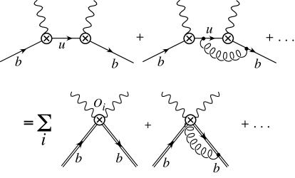
Figure 1: The operator product expansion.

Inclusive quantities may therefore be written as a double expansion in powers of $\Lambda_{\rm QCD}/m_{b}$ (power corrections, from matrix elements of local operators) and $\alpha_{s}(m_{b})$ (perturbative matching corrections).

The OPEs for all inclusive distributions share three important features:

1. The leading term in the $1/m_{b}$ expansion reproduces the free-quark result, as argued on physical grounds. In particular, the kinematics are given by quark, not hadron, masses. This makes inclusive processes sensitive probes of $m_{b}$.

2. The $O(1/m_{b})$ corrections to the parton-model result vanish, owing to the absence of a dimension-four operator that cannot be removed by the equations of motion [21, 22].

3. The leading power corrections to the parton result are proportional to the matrix elements of $\langle B|\bar{b}(iD)^{2}b|B\rangle$ and $\langle B|\bar{b}ig\sigma_{\mu\nu}G^{\mu\nu}b|B\rangle$. These are exactly the parameters $\lambda_{1}$ and $\lambda_{2}$ that entered the relation between $m_{b}$ and $m_{B}$ in Equation 10.

This approach also incorporates an implicit assumption of “quark-hadron duality,” the replacement of the sum over hadron states in Equation 13 with the corresponding sum over parton (quark and gluon) states. The validity of this assumption clearly depends on how inclusive the observable is. For example, the semileptonic $b\to u$ decay rate to hadronic states with invariant mass $m_{X}<m_{\pi}$ obviously vanishes, whereas the corresponding decay rate to free quarks and gluons is nonzero. However, in regions of such severely restricted phase space, the OPE breaks down—the coefficients of both the perturbative and nonperturbative corrections become large—and there is no question of applying it here. The deeper question is whether there are effects due to quark-hadron duality violation that do not show up in the OPE, limiting its accuracy even for more inclusive distributions [25, 26, 27].

Technically, duality violation arises because the OPE is only properly defined in the deep Euclidean region, where the particles that are integrated out are highly off-shell, whereas for inclusive decays the OPE is performed in the Minkowskian region, in which they can go on-shell. Analyticity arguments suggest that extrapolation to the Minkowskian region is valid [19, 20, 21], but they do not provide a rigorous justification. Reference [26] argues that duality violation arises because the expansion in powers of $\Lambda_{\rm QCD}/m_{b}$ in the OPE is asymptotic, and duality-violating effects do not arise at any finite order in $\Lambda_{\rm QCD}/m_{b}$. Reference [25] argues, based on quark models, that such violations could be large, whereas two-dimensional models of QCD [27] suggest that duality violation is a small effect for $B$ decays. Reference [28] concludes from a variety of considerations that duality violation in semileptonic decays is a negligible effect.

Because none of these arguments is truly rigorous, quark-hadron duality should be tested experimentally. The agreement between the $\tau$ hadronic width [20] and the OPE suggests that such corrections may not be large, but consistency among several different predictions of the OPE would bolster one’s confidence that such effects may be neglected.

2.2 NRQCD

Bound states of a heavy quark and antiquark are nonrelativistic systems in the heavy-quark limit. The effective theory to describe such systems is known as nonrelativistic QCD (NRQCD).

Because both NRQCD and HQET correspond to expanding about the $m_{Q}\to\infty$ limit, the operators in the two theories are the same. But because the physics of a nonrelativistic bound state is very different from that of a single heavy quark interacting with light degrees of freedom, the power counting of operators in NRQCD differs from that in HQET.

There are only two important scales in HQET (if we neglect the light-quark masses): the heavy-quark mass, $m_{Q}$, and $\Lambda_{\rm QCD}$. Hence, HQET operators may be classified by their order in $\Lambda_{\rm QCD}/m_{Q}$. In NRQCD, the dynamics depends on two additional scales: the heavy-quark momentum, $p_{Q}=m_{Q}v$, and its kinetic energy, $E_{Q}=\frac{1}{2}m_{Q}v^{2}$ (where $v$ is the relative three-velocity of the two heavy quarks). Because $E_{Q}/m_{Q}$ is the same order in the nonrelativistic expansion as $p_{Q}^{2}/m_{Q}^{2}$, the relevant expansion parameter in NRQCD is not $1/m_{Q}$ but rather the heavy-quark velocity $v$. The velocity scaling rules of NRQCD operators have been worked out [29].

A formulation of NRQCD was proposed by Bodwin, Braaten, and Lepage (BBL) [30], and the analogous theory for electromagnetism, NRQED, had been developed earlier by Caswell & Lepage [31]. The BBL form of the NRQCD Lagrangian is

$${{\cal L}}_{\rm heavy}={\cal L}_{0}+\delta{{\cal L}},$$ (15)

where the leading term is

$${\cal L}_{0}=\psi^{\dagger}\left(iD_{t}+\frac{{\bf D}^{2}}{2m_{Q}}\right)\,\psi,$$ (16)

$\psi(x)$ is a two-component Pauli spinor, and there is a corresponding term for the antiquark field $\chi(x)$. The leading corrections are suppressed by $O(v^{2})$ relative to ${\cal L}_{0}$ and are given by

$$\delta{{\cal L}} = \frac{c_{1}}{8m_{Q}^{3}}\psi^{\dagger}({\bf D}^{2})^{2}\psi+\frac{c_{2}}{8m_{Q}^{2}}\psi^{\dagger}({\bf D}\cdot g{\bf E}-g{\bf E}\cdot{\bf D})\psi$$

$$+ \frac{c_{3}}{8m_{Q}^{2}}\psi^{\dagger}(i{\bf D}\times g{\bf E}-g{\bf E}\times i{\bf D})\cdot\mbox{\boldmath$\sigma$}\psi+\frac{c_{4}}{2m_{Q}}\psi^{\dagger}(g{\bf B}\cdot\mbox{\boldmath$\sigma$})\psi+\dots.$$

The important difference between Equations 15–2.2 and Equations 7–9 is that, in HQET, the heavy-quark kinetic energy is treated as a perturbation, whereas in NRQCD it is leading-order. The correct treatment of the kinetic term is important for describing nonrelativistic Coulomb exchange. For bound states or states near threshold, $v\sim\alpha_{s}$, and Coulomb-exchange graphs proportional to $(\alpha_{s}/v)^{m}$ must be summed to all orders. At leading order in $v$, this is equivalent to solving the nonrelativistic Schrödinger equation. Because NRQCD incorporates relativistic corrections through higher-dimensional operators, it provides an elegant tool for calculating the relativistic corrections to nonrelativistic quantum mechanics, including a correct treatment of radiative corrections and renormalization (which are much more subtle in any other formulation, such as Bethe–Salpeter).

In several proposed alternative formalisms for NRQCD, the scales $m$, $mv$, and $mv^{2}$ are explicitly separated, which is convenient for many purposes [32, 33].

2.3 Lattice QCD

In lattice field theory, the spacetime continuum is replaced by a discrete lattice (see Reference [34] for reviews of lattice QCD). This introduces an ultraviolet cutoff, $p=\pi/a$ (where $a$ is the lattice spacing). The lattice QCD Lagrangian contains, for example, discrete differences, which replace the derivatives of continuum QCD. Because discretization errors are short-distance effects, we can use field-theoretic methods to separate them from the long-distance QCD dynamics. As first proposed by Symanzik [35], EFT can be used to study the effects of the lattice discretization.

Symanzik showed that the lattice theory can be described by a local effective Lagrangian. The leading-order term is simply the continuum QCD Lagrangian. However, the effective theory also contains higher-dimension operators (which are accompanied by the appropriate power of the lattice spacing):

$${{\cal L}}_{\rm eff}={{\cal L}}_{\rm QCD}+a{{\cal L}}_{1}+a^{2}{{\cal L}}_{2}+\ldots,$$ (18)

where ${\cal L}_{\rm QCD}$ is the (Euclidean) continuum QCD Lagrangian,

$${{\cal L}}_{\rm QCD}=-\bar{q}(\mathchoice{\ooalign{$\hfil\displaystyle\mkern 0.0mu/\hfil$\crcr$\displaystyle D$}}{\ooalign{$\hfil\textstyle\mkern 0.0mu/\hfil$\crcr$\textstyle D$}}{\ooalign{$\hfil\scriptstyle\mkern 0.0mu/\hfil$\crcr$\scriptstyle D$}}{\ooalign{$\hfil\scriptscriptstyle\mkern 0.0mu/\hfil$\crcr$\scriptscriptstyle D$}}+m)q\;.$$ (19)

The ${{\cal L}}_{i}$ ($i=1,2,\ldots$) contain operators of dimension $d=4+i$, and all discretization effects of the lattice theory can be described by the ${{\cal L}}_{i}$. The coefficients of the operators in the ${{\cal L}}_{i}$ depend on the underlying lattice theory. Hence, the discretization effects of the lattice theory are organized as a power expansion in the lattice spacing, $a$. The operators typically scale with the momenta of the participating particles in the process, which is $\Lambda_{\rm QCD}$ for light quarks (neglecting quark masses). Hence, we need $a\Lambda_{\rm QCD}\ll 1$ (or more generally, $ap\ll 1$) for the expansion of Equation 18 to be well-behaved. For example, the leading discretization effects of the Wilson action [36] are described by

$${\cal L}_{1}=c_{1}\bar{q}\sigma_{\mu\nu}F^{\mu\nu}q$$ (20)

in the effective theory. A priori, several operators contribute at $O(a)$. However, for the matching between the lattice and effective theories, we need to consider only on-shell quantities [37, 38]. We can therefore use the equations of motion to reduce the number of operators that contribute at any given order of $a$. This leaves only one dimension-five operator in the ${\cal L}_{1}$ term for the Wilson action. In summary, the leading lattice-spacing artifacts of the Wilson action are $O(a\Lambda_{\rm QCD})$ (neglecting quark-mass effects), and we see that the $a\rightarrow 0$ limit recovers continuum QCD from lattice QCD.

This formalism naturally leads us to consider improved formulations of lattice QCD, where operators are added to the lattice QCD Lagrangian so that the coefficients of the leading-order corrections in ${\cal L}_{\rm eff}$ vanish. This procedure is known as Symanzik improvement. For example, we can add a discretized version of the dimension-five operator in Equation 20 to the Wilson action to obtain a lattice action [the Sheikholeslami-Wohlert action [39]] that is correct to $O(a^{2})$, and hence leaves ${\cal L}_{1}=0$. If $n$-loop perturbation theory is used to match the lattice and effective theories, then the $O(a)$ improved action will only be correct up to terms of order $\alpha_{s}^{n+1}a$.

The Symanzik formalism implicitly assumes that $am_{q}\ll 1$, which can be seen explicitly by considering, as an example, the energy-momentum relation obtained from the Wilson or Sheikholeslami-Wohlert actions [40]:

$$E^{2}(\mbox{\boldmath${p}$})=m_{1}^{2}+{m_{1}\over m_{2}}\mbox{\boldmath${p}$}^{2}+O(p^{4}),$$ (21)

where

$${m_{1}\over m_{2}}=1+O(a^{2}m_{1}^{2})$$ (22)

and $m_{1}$ and $m_{2}$ (the rest and kinetic masses, respectively) are functions of the lattice bare mass, $m_{0}$. Although this lattice artifact is suppressed by $a^{2}$, it is large when $am\sim O(1)$. The lattice artifacts that lead to the breakdown can be identified as higher-order terms in the effective Lagrangian of the form $(\gamma_{0}D_{0})^{n}$, with $n>2$. These terms can be eliminated by the field equations [41, 42]:

$$(\gamma_{0}D_{0})^{n}\rightarrow(m_{q}+\mbox{\boldmath${\gamma}$}\cdot\mbox{\boldmath${D}$})^{n}.$$ (23)

We see that when $am_{q}\sim O(1)$, these higher-order terms in the effective Lagrangian are no longer small, and the expansion of Equation 18 breaks down.

With currently practical lattice spacings, $am_{b}>1$. If we don’t want to wait until we have the computational power to reduce the lattice spacing to $am_{b}\ll 1$, we must modify the above prescription to treat $b$-quark mass effects. Because $m_{b}\gg\Lambda_{\rm QCD}$, the $b$-quark mass introduces an additional short-distance scale into the problem, and we should be able to find an effective-theory framework that allows us to lump the short-distance effects from both the lattice spacing and the heavy-quark mass into the coefficients of the effective theory. In fact, there are three solutions to this problem (for a review of lattice methods for heavy quarks, see Reference [43]).

The first solution discretizes the continuum effective theory, either HQET (Equation 7) for the $B$-meson system or NRQCD (Equation 15) for the $b{\bar{b}}$ system. The static theory [44] simply discretizes the leading term in the HQET Lagrangian, Equation 8:

$${\cal L}_{\rm static}=\psi^{\dagger}D_{0}^{\rm lat}\psi\;,$$ (24)

where $D_{0}^{\rm lat}$ is a discretization of the continuum covariant derivative. The leading-order lattice NRQCD Lagrangian is [45]

$${\cal L}_{\rm LNRQCD}=\psi^{\dagger}\left(D_{0}^{\rm lat}-{\Delta^{(2)}\over 2m_{0}}\right)\psi\;,$$ (25)

where $\Delta^{(2)}$ is a discretization of the Laplacian operator. The NRQCD propagators are determined by an evolution equation, which is computationally much simpler to solve than the matrix inversion required by the Dirac propagators. As in the continuum, relativistic corrections can be added to the leading-order term using a discretized version of the correction operators in Equation 2.2. Lattice-spacing errors can be corrected in a similar fashion by adding new operators to the lattice Lagrangian. In this procedure, similar to Symanzik improvement, the coefficients of the correction operators are obtained by matching to the continuum theory. NRQCD is a nonrenormalizable theory, as evidenced by the power-law divergences of some of the coefficients of the NRQCD operators [45]. As a result, the continuum limit ($a\rightarrow 0$) cannot be taken explicitly. Instead, lattice-spacing errors are controlled by adding more terms to the lattice NRQCD Lagrangian until these errors are sufficiently small.

The second solution starts with the observation that the Wilson action has the same heavy-quark symmetries as continuum QCD [40]. Indeed, in the limit $am_{Q}\rightarrow\infty$, the Wilson action reduces to the static limit [44], which corresponds to the leading term in HQET. Hence, instead of matching our relativistic Wilson action to continuum QCD, we can match it to continuum HQET [40, 41]. The difference between the matching for $B$ and $b{\bar{b}}$ systems is the power counting of the operators. In this prescription, the operators of the continuum effective theory are the same as in the usual HQET, as defined, for example, in Equation 7, albeit with different coefficients. All discretization effects are again contained in the coefficients of the operators of the effective Lagrangian. Hence we have a modified HQET of the form [41]

$${\cal L}_{\rm HQET}^{\prime}={\cal L}_{0}^{\prime}+{\cal L}_{1}^{\prime}+...\;,$$ (26)

with

$${\cal L}_{0}^{\prime}=h_{v}(iD\cdot v-m_{1})h_{v}$$ (27)

and

$${\cal L}_{1}^{\prime}={1\over 2m_{2}}\bar{h}_{v}(iD)^{2}h_{v}+{c^{\prime}_{B}\over 2m_{Q}}\bar{h}_{v}\sigma^{\alpha\beta}G_{\alpha\beta}h_{v}\;.$$ (28)

Note that we have incorporated a rest-mass term into the leading-order term of the HQET Lagrangian. This term is usually omitted in the standard HQET prescriptions (see Equation 7). We may add it to our modified HQET Lagrangian, since it has no effect on the dynamics and affects the mass spectrum only additively [15, 45, 46, 41]. The coefficient of the kinetic term in ${\cal L}_{1}$ matches the coefficient of the usual HQET if the lattice quark mass is adjusted so that

$$m_{2}=m_{Q}\;.$$ (29)

The kinetic term in ${\cal L}_{1}^{\prime}$ can easily be matched nonperturbatively, if Equation 29 is imposed on hadron masses. The above prescription demonstrates explicitly that the difference between $m_{1}$ and $m_{2}$ is a lattice artifact that has no effect on the dynamics of the system. These arguments were recently confirmed in a numerical simulation of heavy-quark systems using a relativistic $O(a)$-improved lattice action [47]. In order to adjust the coefficient of the chromomagnetic interaction, $c^{\prime}_{B}$, to its continuum counterpart, we need the $O(a)$ improved Sheikholeslami-Wohlert lattice action. At present, the chromomagnetic operator is matched at tree level only.

In this framework, lattice artifacts arise from the mismatch between the coefficients of higher-dimensional operators of the two effective theories. Just as in the Symanzik formalism, lattice artifacts can either be reduced by brute force (taking $a\rightarrow 0$) or by adding higher-dimensional operators to the lattice action. However, when considering higher-dimensional operators for building improved actions, we must now allow for “nonrelativistic” operators in our lattice action, where spacelike and timelike operators have different coefficients [40].

The third solution is based on the observation that it is possible to match relativistic lattice actions with $am\sim O(1)$ to Equation 18 at the cost of adding an additional parameter to the lattice Lagrangian [40, 42]. This parameter separates timelike and spacelike operators starting at dimension four. With this additional parameter, one can impose $m_{1}=m_{2}$ and recover the relativistic energy-momentum relation. The disadvantage of this method is that it adds an additional parameter that must be adjusted (either perturbatively or nonperturbatively) to recover Equation 18. This method was recently tested in a numerical simulation [47] with good results.

All three solutions discussed above yield lattice QCD formulations that treat heavy-quark–mass effects correctly and allow a systematic analysis of both discretization and heavy-quark–mass effects. Most numerical simulations of heavy-quark systems are based on either the first or the second method discussed above.

3 QUARK-MASS DEFINITIONS

Like any parameter in a Lagrangian, the quark mass is a renormalized quantity and must be appropriately defined by some renormalization condition. In principle, any renormalization condition is allowed; however, some are more convenient to use in a particular calculation than others. In this section, we discuss several renormalization schemes for the $b$-quark mass and highlight their advantages and disadvantages for specific problems.

3.1 The Pole Mass and Renormalons

The simplest quark-mass definition is the pole mass, defined as the solution to

$$\mathchoice{\ooalign{$\hfil\displaystyle\mkern 0.0mu/\hfil$\crcr$\displaystyle p$}}{\ooalign{$\hfil\textstyle\mkern 0.0mu/\hfil$\crcr$\textstyle p$}}{\ooalign{$\hfil\scriptstyle\mkern 0.0mu/\hfil$\crcr$\scriptstyle p$}}{\ooalign{$\hfil\scriptscriptstyle\mkern 0.0mu/\hfil$\crcr$\scriptscriptstyle p$}}-m-\Sigma(p,m)|_{p^{2}=m_{\rm pole}^{2}}=0,$$ (30)

where $\Sigma(p,m)$ is the self energy, in terms of which the full quark propagator is

$$iS(p,m)={i\over\mathchoice{\ooalign{$\hfil\displaystyle\mkern 0.0mu/\hfil$\crcr$\displaystyle p$}}{\ooalign{$\hfil\textstyle\mkern 0.0mu/\hfil$\crcr$\textstyle p$}}{\ooalign{$\hfil\scriptstyle\mkern 0.0mu/\hfil$\crcr$\scriptstyle p$}}{\ooalign{$\hfil\scriptscriptstyle\mkern 0.0mu/\hfil$\crcr$\scriptscriptstyle p$}}-m-\Sigma(p,m)}.$$ (31)

For simplicity, we denote the $b$-quark pole mass by $m_{b}$ in this paper.

The pole mass is the simplest definition to use in HQET and NRQCD, and is related to the meson mass $m_{B}$ via the $1/m_{b}$ expansion in Equation 10. It is gauge-invariant [48] and infrared-finite [49, 50]. However, despite its simplicity, the pole mass has the disadvantage that the perturbation series relating it to physical quantities (such as the decay width) is typically very poorly behaved. For example, the relation between $m_{b}$ and the semileptonic $b\to u$ width is given at two loops by [51, 52]

$$\Gamma(b\rightarrow X_{u}\ell\bar{\nu}_{\ell}) = {G_{F}^{2}|V_{ub}|^{2}m_{b}^{5}\over 192\pi^{3}}\left(1-2.41{\alpha_{s}(m_{b})\over\pi}\right.$$

$$\left.\qquad+\left(3.39-3.22\beta_{0}\right)\left({\alpha_{s}(m_{b})\over\pi}\right)^{2}+\dots\right)$$

$$= {G_{F}^{2}|V_{ub}|^{2}m_{b}^{5}\over 192\pi^{3}}(1-0.17-0.11+\dots)\;,$$

where

$$\beta_{0}\equiv 11-\textstyle{\frac{2}{3}}n_{f}$$ (33)

is the coefficient of the QCD beta function, $n_{f}=4$ is the number of light flavors, the dots denote terms of higher order in $\alpha_{s}$ or $1/m_{b}$, and we have taken $\alpha_{s}(m_{b})=0.22$. The large two-loop term indicates that the perturbation series is poorly behaved, even though $\alpha_{s}(m_{b})/\pi\ll 1$.

This can be seen in a different way by using the prescription of Brodsky, Lepage & Mackenzie (BLM) [53], in which the $O(\alpha_{s}^{2}\beta_{0})$ term is used to determine the appropriate scale for $\alpha_{s}(\mu)$ in the one-loop term. In the BLM prescription, the $O(\alpha_{s}^{2}\beta_{0})$ piece of the two-loop correction (arising from vacuum polarization graphs) is absorbed into the one-loop term by a change of renormalization scale; the resulting scale is taken to be the appropriate renormalization scale of the process. In the case of Equation 3.1, this leads to a scale

$$\mu_{\rm BLM}=m_{b}\exp\left(-{2(3.22)\over 2.41}\right)=0.07\,m_{b}\sim 300\,{\rm{MeV}}.$$ (34)

Since this scale is much lower than the typical momentum transfer in the problem, it indicates a deeper problem.

Bigi et al. and Beneke & Braun have demonstrated [54, 55] that this sickness persists to all orders in perturbation theory. These authors showed that any perturbation series that relates a physical quantity to the pole mass has an intrinsic ambiguity of relative order $\Lambda_{\rm QCD}/m_{b}$ because perturbation theory is only asymptotically convergent [56]. Because $m_{b}$ can be determined only by its relation to a physical quantity, this translates into an ambiguity of the same order in the definition of the pole mass itself. The poor behavior of the series Equation 3.1 even at second order appears to be a reflection of this.

This type of intrinsic ambiguity in perturbation theory is known as an infrared renormalon [57]. Physically, it arises from the low-momentum region of loop integrals where QCD is strongly coupled. Infrared renormalons are ubiquitous in QCD perturbation theory and do not signal an inherent limitation of the theory; in a consistent OPE, there is always a nonperturbative matrix element that enters at the same order in $\Lambda_{\rm QCD}/Q$ as the ambiguity in perturbation theory (where $Q$ is the hard momentum scale in the process), and the sum of perturbative and nonperturbative effects is well-defined [57].

In contrast, the leading nonperturbative term in the expression for the semileptonic $b\to u$ width enters at $O(\Lambda_{\rm QCD}^{2}/m_{b}^{2})$. Hence, it cannot absorb the ambiguity in the series in Equation 3.1, which means that there is an inherent ambiguity of $O(\Lambda_{\rm QCD})$ in the pole mass. The pole mass is particularly sensitive to infrared physics because it is defined as a property of an unphysical on-shell quark. The better-defined mass parameters we discuss in the next section are renormalized at momentum scales much greater than $\Lambda_{\rm QCD}$. Hence, they are insensitive to long-distance physics and do not have this problem.

Rather than discuss the formal theory of infrared renormalons (see Reference [57]), we illustrate their effect with an explicit example. Because it is not feasible to calculate to arbitrarily high order, little has been established rigorously about the asymptotic behavior of QCD perturbation theory. However, a qualitative understanding may be obtained by considering the class of terms proportional to $\alpha_{s}^{n+1}\beta_{0}^{n}$ (the higher-loop analogues of the BLM term). This series is usually simple to compute, since it corresponds to replacing the gluon propagator at one loop with the geometric series shown in Figure 2 and then substituting $n_{f}\to-3\beta_{0}$/2. Note that this is not a well-defined expansion: There is no $\beta_{0}\to\infty$ limit of QCD, and there is no reason that these terms should dominate perturbation theory. However, the series provides a tool to examine high orders of perturbation theory, and barring any miraculous cancellations, we expect the conclusions we draw from this subset of graphs to remain valid in QCD.

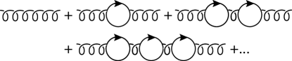
Figure 2: The bubble sum, which may be calculated to arbitrarily high order in perturbation theory.

The techniques to perform the bubble sum were presented in Reference [58]. The series of Equation 3.1 continues (retaining only terms of order $\alpha_{s}^{n}\beta_{0}^{n-1}$) as

$$\Gamma(b\rightarrow X_{u}\ell\bar{\nu}) = {G_{F}^{2}|V_{ub}|^{2}m_{b}^{5}\over 192\pi^{3}}\left[1-2.41{\alpha_{s}\over\pi}+40.5\left({\alpha_{s}(m_{b})\over\pi}\right)^{2}\right.$$

$$\hskip-28.45274pt-820\left({\alpha_{s}(m_{b})\over\pi}\right)^{3}+19192\left({\alpha_{s}(m_{b})\over\pi}\right)^{4}-533495\left({\alpha_{s}(m_{b})\over\pi}\right)^{5}$$

$$\hskip-28.45274pt\left.+1.75\times 10^{7}\left({\alpha_{s}(m_{b})\over\pi}\right)^{6}-6.71\times 10^{8}\left({\alpha_{s}(m_{b})\over\pi}\right)^{7}+\dots\right)$$

$$\hskip-56.9055pt={G_{F}^{2}|V_{ub}|^{2}m_{b}^{5}\over 192\pi^{3}}\left(1-0.15-0.11-0.09-0.09-0.11-0.15-0.25-\dots\right].$$

After several terms, perturbation theory begins to diverge, as expected. The ambiguity in the series is the same size as the smallest term in the series, which a more formal analysis shows to be of order $\Lambda_{\rm QCD}/m_{b}$.

A similar situation arises for the relation between $m_{b}$ and any other physical quantity. For example, the first moment of the hadronic invariant mass spectrum in semileptonic $b\rightarrow u$ decay is related to the pole mass by [59]

$${\langle s_{H}\rangle\over m_{B}^{2}} = 0.202{\alpha_{s}(m_{b})\over\pi}+3.151\left({\alpha_{s}(m_{b})\over\pi}\right)^{2}+51.91\left({\alpha_{s}(m_{b})\over\pi}\right)^{3}$$

$$+940.52\left({\alpha_{s}(m_{b})\over\pi}\right)^{4}+19347.5\left({\alpha_{s}(m_{b})\over\pi}\right)^{5}+{7\over 10}{\bar{\Lambda}\over m_{B}}+\dots\,$$

$$= 0.014+0.015+0.018+0.023+0.032+{7\over 10}{\bar{\Lambda}\over m_{B}}+\dots\,$$

which shows no signs of converging. The dependence of Equation 3.1 on $m_{b}$ is implicit in the ${\bar{\Lambda}}$ term. The two-loop term corresponds to a BLM scale $\mu_{\rm BLM}\simeq 0.03\,m_{b}\sim 100\,{\rm{MeV}}$, and once again an infrared renormalon ambiguity is present at $O(\Lambda_{\rm QCD}/m_{b})$.

However, eliminating $m_{b}$ (or equivalently, $\bar{\Lambda}$) and expressing the two physical quantities $\Gamma$ and $\langle s_{H}\rangle$ in terms of one another results in the much better-behaved relation

$${\langle s_{H}\rangle\over m_{B}^{2}} = -0.135{\alpha_{s}(m_{b})\over\pi}-0.601\left({\alpha_{s}(m_{b})\over\pi}\right)^{2}+1.56\left({\alpha_{s}(m_{b})\over\pi}\right)^{3}$$

$$+148.1\left({\alpha_{s}(m_{b})\over\pi}\right)^{4}+4923.\left({\alpha_{s}(m_{b})\over\pi}\right)^{5}+{7\over 10}{\bar{\Lambda}_{b}^{\Gamma}\over m_{B}}+\dots$$

$$\simeq -0.0086-0.0024+0.0004+0.0026+0.0051+{7\over 10}{\bar{\Lambda}_{b}^{\Gamma}\over m_{B}}+\dots,$$

where $\bar{\Lambda}_{b}^{\Gamma}\equiv m_{B}-(192\pi^{3}\Gamma/G_{F}^{2}|V_{ub}|^{2})^{1\over 5}$ is a physical quantity of order $\Lambda_{\rm QCD}$. [Falk et al.  [59] used this to define the “decay mass” $m_{b}^{\Gamma}\equiv m_{B}-\bar{\Lambda}_{b}^{\Gamma}+O(\Lambda_{\rm QCD}/m_{b}^{2})$, which does not suffer from a renormalon ambiguity.] The convergence of perturbation theory has improved dramatically. It can easilily be shown that the $O(\Lambda_{\rm QCD}/m_{b})$ ambiguity has vanished, and the leading renormalon in Equation 3.1 is now at $O(\Lambda_{\rm QCD}^{2}/m_{b}^{2})$, reflecting the presence of additional unphysical parameters such as $\bar{\Lambda}^{2}$ in the OPE for $\langle s_{H}\rangle$. The corresponding BLM scale is now

$$\mu_{\rm BLM}=0.37\,m_{b}\,\sim 1.8\,{\rm{GeV}},$$ (38)

which is significantly greater than before, and is the natural scale for the process (recall that the energy $m_{b}$ must be divided among several final states, so the typical momentum transfer in the decay is somewhat less than $m_{b}$). The poor behavior of perturbation theory is therefore an artifact of using the pole mass as an unphysical intermediate quantity.

While this is a problem with the pole mass in principle, in practice there is nothing wrong with using it as an intermediate quantity, as long as it is used consistently. However, the presence of the renormalon ambiguity in $m_{b}$ results in pole mass determinations that strongly depend on the order of perturbation theory used in the calculation. Hence, a practical disadvantage of this approach is the difficulty of estimating the theoretical uncertainty in $m_{b}$.

3.2 The ${\overline{\mbox{MS}}}$ Mass

In general, a mass parameter renormalized at a scale $\mu$ is insensitive to physics at longer distance scales. A short-distance mass is not plagued by the infrared problems that afflict the pole mass. An example of such a mass definition in a momentum-subtraction renormalization scheme is the Georgi-Politzer mass, defined at the spacelike subtraction point $-p^{2}=m^{2}$ [60]. However, most analytic perturbative calculations are performed using dimensional regularization. As a result, the most common short-distance mass definition is the ${\overline{\mbox{MS}}}$ mass $\overline{m}_{b}(\mu)$, which is defined by regulating QCD in dimensional regularization and subtracting the divergences in the modified minimal subtraction scheme. The renormalization scale $\mu$ of a short-distance mass is typically chosen to be of the same order as the characteristic energy scale $Q$ of a process, since perturbation theory typically contains terms proportional to $\alpha_{s}^{m}(\mu)\log^{m}(Q/\mu)$, which are otherwise large. The renormalization group may be used to relate a mass renormalized at one scale to that at another scale, summing all the logs of this form to all orders.

The relation between the ${\overline{\mbox{MS}}}$ mass and the pole mass is known to $O(\alpha_{s}^{3})$ [61, 62, 63]:

$${m_{b}\over\overline{m}_{b}} = 1+{4\over 3}{\bar{\alpha}_{s}\over\pi}+\left(1.562\beta_{0}-3.739\right)\left({\bar{\alpha}_{s}\over\pi}\right)^{2}$$

$$+\left(1.4686\beta_{0}^{2}+0.2548\beta_{1}+0.3905\beta_{0}-29.94\right)\left({\bar{\alpha}_{s}\over\pi}\right)^{3}+O(\alpha_{s}^{4}),$$

where

$$\beta_{1}\equiv 102-\frac{38}{3}n_{f}$$ (40)

and we use the notation

$$\overline{m}_{b}\equiv\overline{m}_{b}(\overline{m}_{b}),$$ (41)

where $\overline{m}_{b}(\overline{m}_{b})$ is the ${\overline{\mbox{MS}}}$ mass renormalized at the scale $\mu=\overline{m}_{b}(\mu)$ and $\bar{\alpha}_{s}\equiv\alpha_{s}(\overline{m}_{b})$. All light quarks have been treated as massless in this expression. The complete $m_{c}$ dependence of the $O(\alpha_{s}^{2})$ term is known [61], and the $O(\alpha_{s}^{3}m_{c})$ terms have been calculated [64].

The ${\overline{\mbox{MS}}}$ mass $\overline{m}_{b}(\mu)$ arises naturally in high-energy processes, such as $Z\to b{\bar{b}}$, in which the $b$ quarks are produced relativistically. For example, the contribution of the axial current to the decay $Z\to b{\bar{b}}X$ is [65]

$$\Gamma_{Z}^{A} = {Gm_{Z}^{3}\over 8\sqrt{2\pi}}a_{b}^{2}\left\{1+{\alpha_{s}\over\pi}-6{m_{b}^{2}\over m_{Z}^{2}}\left[1+{\alpha_{s}\over\pi}\left(1-2\ln{m_{Z}^{2}\over m_{b}^{2}}\right)\right]+\dots\right\}$$

$$= {Gm_{Z}^{3}\over 8\sqrt{2\pi}}a_{b}^{2}\left\{1+{\alpha_{s}\over\pi}-6{\overline{m}_{b}(\mu)^{2}\over m_{Z}^{2}}\left[1+{\alpha_{s}\over\pi}\left(1-2\ln{m_{Z}^{2}\over\mu^{2}}+\frac{11}{3}\right)\right]+\dots\right\}.$$

In the pole mass scheme, the large logarithm of $m_{Z}^{2}/m_{b}^{2}$ makes perturbation theory artificially badly behaved; choosing the ${\overline{\mbox{MS}}}$ mass renormalized at a scale $\mu\sim m_{Z}$ eliminates the large logarithm.

However, the ${\overline{\mbox{MS}}}$ mass is less useful for heavy quarks at nonrelativistic energies. Trading the pole mass for $\overline{m}_{b}$ only slightly improves the apparent convergence of perturbation theory for the semileptonic $b$ width at two loops [51],

$$\Gamma(b\rightarrow X_{u}\ell\bar{\nu}) = \Gamma_{0}\overline{m}_{b}^{5}\left(1+4.25{\alpha_{s}(m_{b})\over\pi}+4.58\left({\alpha_{s}(m_{b})\over\pi}\right)^{2}\beta_{0}+\dots\right)$$ (43)

$$\simeq \Gamma_{0}\overline{m}_{b}^{5}\left(1+0.30+0.19+\dots\right),$$

corresponding to a BLM scale $\mu_{\rm BLM}\simeq 0.12\,m_{b}\sim 500\,{\rm{MeV}}$. However, the asymptotic behavior of the series improves, and indeed it can be shown that the $O(\Lambda_{\rm QCD})$ ambiguity vanishes in this relation.

Because the typical momentum transfer in semileptonic $b$ decays is somewhat less than $m_{b}$, it might be argued that the appropriate mass to use is $\overline{m}_{b}(\mu)$, where $\mu<m_{b}$. Indeed, Reference [66] stressed that the appropriate renormalization point for $b\to u$ semileptonic decay is $m_{b}/n$, where $n=5$ is the power of $m_{b}$ in the total semileptonic width. However, as emphasized in Reference [66], the ${\overline{\mbox{MS}}}$ mass is not a useful quantity when renormalized at a scale $\mu<m_{b}$. From the effective-theory perspective, this is easy to see; the ${\overline{\mbox{MS}}}$ mass is defined in full QCD, treating the $b$ quark as fully dynamical. This is the appropriate theory to calculate the running of the ${\overline{\mbox{MS}}}$ mass from some high scale down to $m_{b}$. At the scale $\mu=m_{b}$, however, the effective theory changes from QCD to HQET. It therefore makes no sense to lower $\mu$ beyond $m_{b}$ in full QCD, and in HQET the pole mass does not run. Renormalizing $\overline{m}_{b}(\mu)$ below this scale simply introduces spurious logarithms that have no physical significance, and therefore do not improve the convergence of perturbation theory. Thus, although the ${\overline{\mbox{MS}}}$ mass is at least well-defined, it is not a particularly useful quantity to relate to low-energy observables.

3.3 Threshold Masses

Because of the shortcomings of the pole and ${\overline{\mbox{MS}}}$ masses for describing the physics of nonrelativistic heavy quarks, several alternative mass definitions have been suggested, which we group here under the term “threshold masses” (following Reference [67]). These are mass definitions for which the $O(\Lambda_{\rm QCD}/m_{b})$ renormalon is absent, but which have better-behaved perturbative relations to properties of nonrelativistic heavy quarks than the ${\overline{\mbox{MS}}}$ mass. One may define an arbitrary number of sensible mass parameters, but several definitions have become popular in the literature, and we now consider them in turn.

3.3.1 The Kinetic Mass

The kinetic mass $m_{b}^{\rm{kin}}(\mu_{f})$ introduced by Bigi and collaborators [68, 66, 69] is defined by introducing an explicit factorization scale $\mu_{f}$, and subtracting the physics at scales below $\mu_{f}$ from the quark-mass definition.

More explicitly, the kinetic mass is defined by considering various sum rules for semileptonic $b\to c$ decay in the small velocity (SV) limit [9], $m_{b},m_{c}\gg m_{b}-m_{c}\gg\Lambda_{\rm QCD}$. In this limit, the charmed meson is produced with vanishingly small recoil ($m_{c}\gg m_{b}-m_{c}$), but there is still enough energy transfer to produce a large number of excited charmed states ($m_{b}-m_{c}\gg\Lambda_{\rm QCD}$), so that the decay may be treated inclusively. In this limit, one can derive sum rules that relate $\bar{\Lambda}$ and $\lambda_{1}$ (and higher-order terms if required) to weighted integrals of the spectral function. By putting an explicit cutoff $\mu_{f}$ on the integrals, Bigi et al. define a cutoff $\bar{\Lambda}(\mu_{f})$ and $\lambda_{1}(\mu_{f})$ that determine the kinetic mass via (compare with Equation 10)

$$m_{B}=m_{b}^{\rm{kin}}(\mu_{f})+\bar{\Lambda}(\mu_{f})-{\lambda_{1}(\mu_{f})\over 2m_{b}^{\rm{kin}}(\mu_{f})}+\dots,$$ (44)

where the $\lambda_{2}$ term and terms of higher order in $1/m_{b}$ have been neglected. In the limit $\mu_{f}\to 0$, the pole mass is regained, whereas for $\Lambda_{\rm QCD}\ll\mu_{f}\ll m_{b}$, this definition removes the dangerous low-momentum region from the definition of $m_{b}^{\rm{kin}}(\mu_{f})$ and therefore eliminates the infrared renormalon ambiguity while leaving the heavy-quark expansion valid.

The relation between the kinetic mass and the ${\overline{\mbox{MS}}}$ mass is known to two loops [70]:

$$m_{b}^{\rm{kin}}(\mu_{f}) = \overline{m}_{b}\left\{1+{4\over 3}{\bar{\alpha}_{s}\over\pi}\left(1-{4\over 3}{\mu_{f}\over\overline{m}_{b}}-{\mu_{f}^{2}\over 2\overline{m}_{b}^{2}}\right)+\left({\bar{\alpha}_{s}\over\pi}\right)^{2}\left[K-{8\over 3}\right.\right.$$ (45)

$$\left.\left.\hskip-28.45274pt+{\mu_{f}\over\overline{m}_{b}}\left({8\beta_{0}\over 9}X_{1}+{8\pi^{2}\over 9}-{52\over 9}\right)+{\mu_{f}^{2}\over\overline{m}_{b}^{2}}\left({\beta_{0}\over 3}X_{2}+{\pi^{2}\over 3}-{23\over 18}\right)\right]\right\},$$

where

$$K={\beta_{0}\over 2}\left({\pi^{2}\over 6}+{71\over 48}\right)+\frac{665}{144}+\frac{\pi^{2}}{18}\left(2\ln 2-\frac{19}{2}\right)-\frac{1}{6}\zeta_{3},$$ (46)

$$X_{1}=\log\frac{2\mu_{f}}{\overline{m}_{b}}-\frac{8}{3},\ \ X_{2}=\log\frac{2\mu_{f}}{\overline{m}_{b}}-\frac{13}{6}\,,$$ (47)

and terms of order $\mu_{f}^{3}/m_{b}^{3}$ and higher have been neglected.

3.3.2 The Potential-Subtracted Mass

The potential-subtracted (PS) mass proposed in Reference [71] has similar properties to the kinetic mass, but arises from consideration of the properties of nonrelativistic quark-antiquark systems.

The dynamics of heavy quarkonium are determined by the Schrödinger equation,

$$\left(-{\nabla^{2}\over m_{b}}+V(r)-E\right)G(\vec{r},0,E)=\delta^{(3)}(\vec{r}),$$ (48)

where $E\equiv\sqrt{s}-2m_{b}$ is the binding energy and $V(r)$ is the static QCD potential. This expression includes the total static energy of two heavy quarks at a distance $r$ [72, 71],

$$E_{\rm stat}(r)=2m_{b}+V(r).$$ (49)

Because this is a physical quantity, it is well-defined and should not suffer from a renormalon ambiguity. Indeed, the high-order behavior of $V(r)$ has been shown to precisely cancel that of the pole mass, so that the combination of Equation 49 is well-defined. The infrared sensitivity of the long-distance quark-antiquark potential exactly cancels that of the pole mass.

This cancellation is made explicit by eliminating the pole mass in terms of the so-called potential-subtracted (PS) mass. The coordinate-space potential is defined as the Fourier transform of the momentum-space potential,

$$V(r)=\int{d^{3}q\over(2\pi)^{3}}e^{iq\cdot r}\widetilde{V}(q).$$ (50)

As noted in Reference [71], the coordinate-space potential is more sensitive to infrared physics than the momentum-space potential because of the contribution to the Fourier integral from the region of small $|q|$, and this region was identified as the source of the leading renormalon in $V(r)$. In the PS scheme, this contribution is subtracted from the potential and instead included in the mass through the definitions

$$m_{b}^{\rm PS}(\mu_{f})=m_{b}-\delta m(\mu_{f}),\ \ \ V(r,\mu_{f})=V(r)+2\delta m(\mu_{f}),$$ (51)

where

$$\delta m=-{1\over 2}\int_{|\vec{q}|<\mu_{f}}{d^{3}\vec{q}\over(2\pi)^{3}}\tilde{V}(q)\;.$$ (52)

Using the PS mass and subtracted potential in the Schrödinger equation thus results in a better-behaved perturbation series for the quark mass.

The relation between $m_{b}^{\rm PS}$ and $m_{b}$ is known to three loops [71]:

$$m_{b}^{\rm PS}(\mu_{f}) = m_{b}-{\alpha_{s}(\mu)C_{F}\over\pi}\mu_{f}\left\{1+{\alpha_{s}(\mu)\over 4\pi}\left[a_{1}-\beta_{0}\left(\ln{\mu_{f}^{2}\over\mu^{2}}-2\right)\right]\right.$$ (53)

$$+\left.\left(\alpha_{s}(\mu)\over 4\pi\right)^{2}\left[a_{2}-(2a_{1}\beta_{0}+\beta_{1})\left(\ln{\mu_{f}^{2}\over\mu^{2}}-2\right)\right.\right.$$

$$+\left.\left.\beta_{0}^{2}\left(\ln^{2}{\mu_{f}^{2}\over\mu^{2}}-4\ln{\mu_{f}^{2}\over\mu^{2}}+8\right)\right]\right\}.$$

where

$${}a_{1} = \frac{31}{9}C_{A}-\frac{20}{9}T_{R}n_{f}=\frac{31}{3}-\frac{10}{9}n_{f}$$

$$a_{2} = \left(\frac{4343}{162}+4\,\pi^{2}-\frac{\pi^{4}}{4}+\frac{22}{3}\,\zeta_{3}\right)C_{A}^{2}-\left(\frac{1798}{81}+\frac{56}{3}\zeta_{3}\right)C_{A}T_{R}n_{f}$$ (54)

$$-\left(\frac{55}{3}-16\zeta_{3}\right)C_{F}T_{R}n_{f}+\left(\frac{20}{9}T_{R}n_{f}\,\right)^{2}$$

$$= 653.71-66.354n_{f}+1.2346n_{f}^{2}$$

and $C_{A}=3$, $C_{F}=4/3$, $T_{R}=1/2$. The constant $a_{2}$ depends on the three-loop static potential and was calculated in Reference [74]. Combining Equations 53 and 3.2 gives the three-loop relation between $m_{b}^{\rm PS}$ and $\overline{m}_{b}$.

Note that for the appropriate choice $\mu_{f}\ll m_{b}$, both the kinetic mass and the PS mass may be made to differ from the pole mass by $O(m_{b}v^{2})$. This is important for power counting in Coulomb systems, since this is the same size as the Coulomb binding energy. For both nonrelativistic $b\bar{b}$ problems and $B$ decays, the scale $\mu_{f}\sim 1\,{\rm{GeV}}$ gives well-behaved series.

3.3.3 The $1S$ Mass

Both the kinetic and PS masses are defined by introducing an explicit factorization scale $\mu_{f}$ to remove the troublesome infrared physics of the pole mass. In constrast, the $1S$ mass introduced in References [75] and [76], which we denote here by $m_{b}^{1S}$, achieves a similar goal without introducing a factorization scale. However, the renormalon cancellation is subtle in this case, and the $1S$ mass is a well-behaved parameter only if the orders of terms in perturbation theory are reinterpreted [75].

The $1S$ mass is simply defined as one half the energy of the $1S$ $b\bar{b}$ state, calculated in perturbation theory. To three loops [77],

$${m_{b}^{1S}\over m_{b}} = 1-{(\alpha_{s}(\mu)C_{F})^{2}\over 8}\left\{1+{\alpha_{s}(\mu)\over\pi}\left[\beta_{0}(\ell+1)+\frac{a_{1}}{2}\right]\right.$$

$$+ \left({\alpha_{s}(\mu)\over\pi}\right)^{2}\left[\beta_{0}^{2}\left(\frac{3}{4}\ell^{2}+\ell+\frac{\zeta_{3}}{2}+\frac{\pi^{2}}{24}+\frac{1}{4}\right)+\beta_{0}\frac{a_{1}}{2}\left(\frac{3}{2}\ell+1\right)\right.$$

$$\left.\left.+\frac{\beta_{1}}{4}(\ell+1)+\frac{a_{1}^{2}}{16}+\frac{a_{2}}{8}+\left(C_{A}-\frac{C_{F}}{48}\right)C_{F}\pi^{2}\right]+\ldots\right\},$$

where

$$\ell \equiv \ln\left(\frac{\mu}{C_{F}\alpha_{s}(\mu)m_{b}}\right)$$ (56)

and the other parameters are defined in Equation 3.3.2. Note that $m_{b}^{1S}$ is renormalization-group-invariant.

In the large $\beta_{0}$ limit, the series of Equation 3.3.3 contains terms of order

$$\alpha_{s}^{2},\alpha_{s}^{3}\beta_{0},\alpha_{s}^{4}\beta_{0}^{2},\dots\ \ ,$$

whereas perturbation theory typically contains terms of order

$$\alpha_{s},\alpha_{s}^{2}\beta_{0},\alpha_{s}^{3}\beta_{0}^{2},\dots\ \ .$$

This apparent mismatch makes it unclear how the use of the $1S$ mass will improve the convergence of perturbation theory. However, as shown in Reference [75], at high orders in perturbation theory the coefficient of $\alpha_{s}^{n+2}\beta_{0}^{n}$ in the continuation of Equation 3.3.3 contains terms of the form $(\ell^{n}+\ell^{n-1}+\dots+1)$, which exponentiate at large $n$ to $\exp(\ell)=\mu/(m_{b}\alpha_{s}C_{F})$. This factor corrects the mismatch between powers of $\alpha_{s}$ and $\beta_{0}$ (at least at large orders in perturbation theory), allowing the renormalon ambiguities to cancel between Equation 3.3.3 and other perturbation series. This observation led Hoang et al.  [75] to propose the so-called Upsilon expansion. In this approach, terms in the perturbative expansion of the $1S$ mass of order $\alpha_{s}^{n}$ are formally taken to be of the same order as those of order $\alpha_{s}^{n-1}$ in other series. To make this manifest, a power-counting parameter $\epsilon=1$ is introduced, and terms of $O(\alpha_{s}^{n})$ in the $1S$ mass are multiplied by $\epsilon^{n-1}$, while those in other series are multiplied by $\epsilon^{n}$. When combining series, terms of the same order in $\epsilon$ are combined.

Using this approach, the $1S$ mass has been shown to have remarkably well-behaved perturbative relations to other physical quantities. For example, the $b\to u$ semileptonic width is given by

$$\Gamma(b\to X_{u}\ell\bar{\nu}_{\ell})={G_{F}^{2}|V_{ub}|^{2}(m_{b}^{1S})^{5}\over 192\pi^{3}}\left(1-0.115\epsilon-0.035\epsilon_{\rm BLM}^{2}+\dots\right),$$ (57)

where we have taken $\alpha_{s}(m_{b})=0.22$, and $\epsilon^{2}_{\rm BLM}$ denotes only the terms of order $\epsilon^{2}$ enhanced by $\beta_{0}$.

3.4 Lattice Quark Masses

Almost all determinations of the $b$-quark mass from lattice QCD use lattice perturbation theory to calculate the $b$ quark’s self energy. A few general comments on lattice perturbation theory are therefore given in Section 3.4.1, which also defines the conventions used in the following discussion.

Before we discuss the specific strategies for $b$-quark-mass determinations, we briefly review how (light) quark masses are determined from lattice QCD in general. The quark masses are adjustable parameters in the lattice QCD Lagrangian. One then calculates a suitable hadron mass on the lattice and adjusts the lattice quark mass until the lattice result agrees with the experimentally measured value. A suitable hadron is one that is easily and reliably calculable from lattice QCD. Because they have fewer valence quarks, mesons are simpler to simulate than baryons. Mesons that are stable under the strong interactions are less affected by sea-quark effects, the incomplete inclusion of which often causes the dominant error. Hence, in light-quark systems, the pion and kaon masses are generally used for quark-mass determinations. For the $b$ quark, the most suitable hadrons are the (spin-averaged) $B$ and $B_{s}$ mesons and the $\Upsilon$ system.

The procedure described above yields a nonperturbative determination of the lattice quark mass as it appears in the lattice QCD Lagrangian, which is used in the numerical simulation. Lattice quark masses, though well-defined and free of renormalon ambiguities, are not very useful parameters in continuum calculations. For light quarks, the relation between the lattice and $\overline{\rm MS}$ mass is known at one loop (for all light-quark actions used in numerical simulations):

$$\overline{m}(\mu)=Z_{m}^{\overline{\rm MS}}(\mu)\,m_{0}$$ (58)

with

$$Z_{m}^{\overline{\rm MS}}(\mu)=1+{\alpha_{P}(q^{*})\over 4\pi}(c^{(0)}+\gamma^{0}\ln(\mu a)^{2}+\ldots).$$ (59)

The value of $c^{(0)}$ depends on the lattice action, and $\gamma^{0}$ is the anomalous dimension at leading order. Several groups have introduced procedures for nonperturbatively determining renormalized quark masses. These procedures avoid the perturbative uncertainty of Equation 58 but must still deal with lattice-spacing and other systematic uncertainties. One example is the renormalization-group–invariant (RGI) mass as defined in Reference [78]. One needs perturbation theory to obtain $\overline{m}$ from the RGI mass. Because the relation is known at four-loop order and the matching can be done at a very high-energy scale, the conversion of the RGI mass to $\overline{m}$ introduces only a small additional uncertainty.

There are several different strategies for lattice determinations of the $b$-quark mass. The first method is similar in spirit to light-quark mass determinations. One calculates the kinetic mass, the coefficient of the kinetic term in the energy-momentum relation. Nonrelativistically,

$$E(\mbox{\boldmath${p}$})=E(0)+{1\over 2M_{\rm kin}}\mbox{\boldmath${p}$}^{2}+\ldots.$$ (60)

The dispersion relation of Equation 60 is applied to the hadron system, and the lattice quark mass, $m_{0}$, is tuned until the lattice calculation of $M_{\rm kin}$ agrees with its corresponding experimental result.

As discussed above, this procedure yields a nonperturbative determination of the lattice quark mass, $m_{0}$, which can be related to the $\overline{\rm MS}$ mass in perturbation theory. This relation is generally known at one-loop order:

$$\overline{m}_{b}(\mu)=m_{0}\left(1+c^{(1)}(\mu){\alpha_{P}(q^{*})\over\pi}+\ldots\right),$$ (61)

where $c^{(1)}(\mu)$ depends, as usual, on the lattice action, and the renormalization scheme and scale of the coupling. Numerically, $c^{(1)}$ is $O(1)$.

In the second method, the $b$-quark pole mass is determined from lattice QCD calculations of the binding energy. For the $B$-meson system, we have

$$m_{b}=\overline{M}^{\rm exp}-{\cal E}\;,$$ (62)

where $\overline{M}^{\rm exp}$ is the spin average of the experimentally measured $B$ and $B^{*}$ masses, and the binding energy ${\cal E}$ is obtained from

$${\cal E}=E_{\rm lat}-E_{0}\;.$$ (63)

$E_{\rm lat}$ is the binding energy in the $B$-meson system calculated from a numerical lattice NRQCD or HQET simulation. $E_{0}$ is the $b$ quark’s nonrelativistic self energy, which depends on the underlying lattice NRQCD (or HQET) action. It is a short-distance quantity and hence calculable in perturbation theory. In calculations with relativistic heavy-quark lattice actions (which contain an explicit rest mass term), Equation 63 is modified to

$${\cal E}=\overline{M}_{1,\rm lat}-m_{1}\;,$$ (64)

where $\overline{M}_{1,\rm lat}$ is the spin-averaged rest mass of the $B$-meson as calculated from lattice QCD and $m_{1}$ is the lattice heavy quark’s rest mass (defined in Section 2.3), which is again calculable in perturbation theory.

Both $E_{0}$ and $m_{1}$ have been calculated to one-loop order in perturbation theory [80, 81], for example,

$$E_{0}={e_{0}\over a}\alpha_{P}+O(\alpha_{P}^{2})\;.$$ (65)

Calculations of the two-loop corrections for both $E_{0}$ and $m_{1}$ are currently in progress (H. Trottier, private communication), and we expect these results to become available soon. Once the two-loop results are available, it should be possible to estimate the three-loop correction, using a numerical technique that has been succcessfully used to determine the three-loop correction for the static self energy [82] (see Equation 66 below). The coefficient $e_{0}$ in Equation 65 depends on the lattice NRQCD action used in the numerical calculation, and on the renormalization scale (and scheme) of the coupling. It also depends mildly on the lattice quark mass. The power-law divergences present in both $E_{0}$ and the numerically calculated $E_{\rm lat}$ cancel, leaving the binding energy ${\cal E}$ divergence free.

In the static limit, the $b$ quark’s self energy was until recently known only to two-loop order [83, 79]. The three-loop coefficient has now been calculated by two groups [84, 82] using different numerical techniques:

$$E_{0}^{\infty}=1.0701\,\alpha_{P}(0.84/a)+0.117\,\alpha_{P}^{2}+(3.56\pm 0.50)\alpha_{P}^{3}+O(\alpha_{P}^{4})\;.$$ (66)

The $n_{f}$ dependence of the two-loop coefficient is known; reported here are the values at $n_{f}=0$ (in the quenched approximation). The coefficient of the $\alpha_{P}^{3}$ term is only known at $n_{f}=0$.

Comparing Equation 62 to Equation 10, we see that a lattice calculation of the binding energy, ${\cal E}$, can be used to determine the HQET parameters, ${\bar{\Lambda}}$, $\lambda_{1}$ (and $\lambda_{2}$) [85]:

$${\cal E}={\bar{\Lambda}}-{\lambda_{1}\over 2m_{\rm kin}}+O(1/m^{2}).$$ (67)

Here $1/2m_{\rm kin}$ is a short-distance coefficient defined from the heavy quark’s energy momentum relation as in (for example) Equation 21 or Equation 60. The term $\lambda_{2}$ drops out of this equation, since ${\cal E}$ in Equation 62 is calculated from the spin average of the $B$ and $B^{*}$ masses. It can be determined separately by considering the $B^{*}$-$B$ mass difference.

For the $b{\bar{b}}$ system, Equations 62–64 must be modified to account for the two heavy quarks in the bound state:

$$m_{b}=\textstyle{\frac{1}{2}}(M_{\Upsilon}^{\rm exp}-{\cal E})$$ (68)

and

$${\cal E}=E_{\rm lat}-2E_{0}\;{\rm or}\;\;{\cal E}=\overline{M}_{1,\rm lat}-2m_{1}\;.$$ (69)

In either case, the pole mass determined from Equation 62 (or Equation 68) can be converted to any other continuum mass defined in the previous subsections, using the relations given there. The renormalon ambiguity present in the pole mass manifests itself in the perturbative expansion of $E_{0}$ (or $m_{1}$). If one uses, for example, Equation 3.2 to relate the pole mass to the $\overline{\rm MS}$ mass, then the renormalon ambiguities in Equation 3.2 and 62 will cancel, leaving a well-defined perturbative expansion. In order to make this cancellation explicit, one should use the same coupling in both equations.

3.4.1 Lattice Perturbation Theory

The previous section shows that lattice perturbation theory is often a necessary ingredient in quark-mass determinations. However, perturbative expansions expressed in terms of the bare lattice coupling are not well-behaved. For example, the static self energy of Equation 66 expressed in terms of the bare lattice coupling, $\alpha_{\rm lat}$, takes the form

$$E_{0}^{\infty}=2.1173\,\alpha_{\rm lat}+11.152\,\alpha_{\rm lat}^{2}+(86.2\pm 0.5)\,\alpha_{\rm lat}^{3}+O(\alpha_{\rm lat}^{4})\;.$$ (70)

The perturbative series in Equation 70 looks very divergent, with increasing coefficients. However, as explained in Reference [86], this is an artifact of using a poor expansion parameter. The reliability of lattice perturbation theory is easily tested by comparing short-distance quantities calculated in Monte Carlo simulations to their perturbative expressions. As discussed in Reference [86], even two-loop predictions fail miserably at reproducing Monte Carlo results for short-distance quantities if the perturbative results are expressed in terms of the bare lattice coupling. If instead the perturbative results are expressed in terms of a renormalized coupling (such as $\alpha_{V}$ or $\alpha_{\overline{\rm MS}}$), then perturbative and Monte Carlo results are in good agreement. The accuracy of perturbative predictions is further improved if the scale at which the coupling is evaluated in the perturbative expansion corresponds to the typical momentum scale of the gluons in the physical quantity.

We follow the procedure suggested in Reference [86], which is particularly convenient for lattice perturbation theory and has been shown to produce reliable perturbative estimates. We define the coupling $\alpha_{P}$ from the expectation value of the plaquette (the smallest Wilson loop on the lattice):

$$-\ln{\langle{\rm Tr}\,U_{P}\rangle}\equiv{4\pi\over 3}\alpha_{P}(3.40/a)(1-1.1909\,\alpha_{P})\,.$$ (71)

The coupling $\alpha_{P}$ is defined so that the perturbative expansion of the plaquette in terms of $\alpha_{P}$ contains no higher-order terms. The definition of $\alpha_{P}$ is designed to coincide with the coupling defined from the heavy-quark potential in momentum space,

$$V(q)=-{C_{f}4\pi\alpha_{V}(q)\over q^{2}}\;,$$ (72)

through one-loop order,

$$\alpha_{P}=\alpha_{V}+O(\alpha_{V}^{3})\;.$$ (73)

The scale $q^{*}$ at which the coupling is evaluated is defined as

$$\ln({q^{*}}^{2})\equiv\frac{\int d^{4}qf(q)\ln(q^{2})}{\int d^{4}qf(q)}\;,$$ (74)

where $f(q)$ is the integrand of the quantity that is evaluated at one loop. This definition for setting the scale is very similar in spirit to the BLM procedure for continuum perturbation theory.

This procedure turns the perturbative expansion of Equation 70 into the much better-behaved Equation 66.

4 DETERMINATIONS OF THE $b$-QUARK MASS

4.1 The $b{\bar{b}}$ System

The $\Upsilon$ system has historically been an important source of information on $m_{b}$. As discussed in Section 1, potential models provide a good fit to the observed spectrum of $b{\bar{b}}$ resonances and give model-dependent determinations of $m_{b}$. More recently, there have been model-independent determinations of $m_{b}$ from the masses of the low-lying resonances as well as from the near-threshold behavior of the $e^{+}e^{-}\to b{\bar{b}}X$ cross section. All of these determinations use the fact that $b{\bar{b}}$ states are nonrelativistic, and therefore can, to first order, be described by the nonrelativistic Schrödinger equation. Effective field theory is then typically used to calculate both relativistic and nonperturbative corrections to this limit.

In this section, we discuss determinations of $m_{b}$ from the $\Upsilon(1S)$ mass using both calculations based on perturbation theory and those from lattice QCD. We also discuss determinations of $m_{b}$ from $\Upsilon$ sum rules.

4.1.1 The $\Upsilon(1S)$ Mass

In the heavy-quark limit, the $b\bar{b}$ pair form a nonrelativistic Coulomb bound state with dynamics determined by the Schrödinger equation. Thus, in the heavy-quark limit it is straightforward to determine $m_{b}$ from the spectrum of $\Upsilon$ mesons. For sufficiently heavy quarkonium,

$$m_{\Upsilon(nS)}=m_{\Upsilon(nS)}^{\rm pert}+\delta M_{\Upsilon(nS)}^{\rm NP},$$ (75)

where $m_{\Upsilon(nS)}^{\rm pert}$ is calculable in perturbation theory and $\delta M_{\Upsilon(nS)}^{\rm NP}$ denotes the nonperturbative contribution to the $\Upsilon$ mass. This immediately gives the result

$$m_{b}^{1S}=4.73\,{\rm{GeV}}-\textstyle{\frac{1}{2}}\delta M_{\Upsilon(1S)}^{\rm NP}$$ (76)

or

$$\overline{m}_{b}=4.21\,{\rm{GeV}}\pm\mbox{nonperturbative\ corrections}.$$ (77)

The trick is to determine the size of the nonperturbative corrections.

Potential-model studies indicate that the $\Upsilon$ system is far from a Coulomb bound state; the radius of even the lowest lying states sits squarely in the confining potential, which suggests that nonperturbative effects are important for these states. [More recently, Brambilla et al. [87] showed that this may merely reflect the use of the poorly defined pole mass in the potential model. These authors find that perturbation theory expressed in terms of a short-distance mass gives a good fit to the $\Upsilon(1S)$, $\chi(1P)$, and $\Upsilon(2S)$ levels of bottomium.] Voloshin [88] and Leutwyler [89] showed years ago that the leading nonperturbative corrections to the heavy-quark limit cannot be absorbed in a nonperturbative potential. Rather, in the heavy-quark limit a $b{\bar{b}}$ bound state is a compact object of size $\ll 1/\Lambda_{\rm QCD}$, and nonperturbative effects correspond to the interaction of the QCD vacuum with the multipole moments of the bound state. Furthermore, the correlation time for the background gluon field $\sim 1/\Lambda_{\rm QCD}$ must also be much greater than the dynamical timescale for the quarkonium state $\sim 1/m_{b}v^{2}$, where $v\sim\alpha_{s}(m_{b}v)$ is the typical velocity of the $b$ quark in the meson.

In this limit, the nonperturbative correction $\delta M_{\Upsilon(nS)}^{\rm NP}$ may be written as a series in terms of local condensates [88, 89, 90]:

$$\delta M_{\Upsilon(nS)}^{\rm NP}\sim\sum_{r=0}^{\infty}C_{r}\,{m_{b}v^{2}\over n^{2}}\left({\Lambda_{\rm QCD}n^{2}\over m_{b}v}\right)^{2}\left({\Lambda_{\rm QCD}n^{2}\over m_{b}v^{2}}\right)^{2r+2}.$$ (78)

The obvious difficulty with treating the $b\bar{b}$ system in this approach is that the inequality

$$m_{b}\alpha_{s}^{2}(m_{b}v)\gg\Lambda_{\rm QCD}$$ (79)

does not hold; both sides are of order a few hundred MeV. Nevertheless, because the leading operator only arises at $O(\Lambda_{\rm QCD}^{4})$, taking the OPE at face value gives a rather small correction to the $\Upsilon(1S)$ mass from the first condensate,

$$\delta M_{\Upsilon(1S)}^{\rm NP}=\textstyle{\frac{624}{425}}\pi m_{b}{\langle 0|\alpha_{s}G^{a\mu\nu}G^{a}_{\mu\nu}|0\rangle\over\left(m_{b}C_{F}\alpha_{s}\right)^{4}}+\dots\simeq 90\,{\rm{MeV}},$$ (80)

using $\langle 0|\alpha_{s}G^{a\mu\nu}G^{a}_{\mu\nu}|0\rangle=0.05\,{\rm{GeV}}^{4}$ [91] and evaluating $\alpha_{s}$ at the Bohr radius of the $1S$ state. This is a reasonably small contribution, even though the inequality of Equation 79 is not well satisfied. The more realistic scaling

$$m_{b}v\gg m_{b}v^{2}\sim\Lambda_{\rm QCD}$$ (81)

is much more difficult to describe theoretically. The corresponding corrections to the heavy-quark limit are given by condensates that are nonlocal in time, about which very little is known [92].

Because Equation 80 is not expected to dominate the series in Equation 78 for physical values of the $b$-quark mass, it is not clear how sensible this estimate of the nonperturbative corrections is. References [75, 93] and [94] take Equation 80 as indicative of the size of nonperturbative corrections and treat it as an estimate of the theoretical error rather than a correction. Beneke & Signer [93] then determine

$$m_{b}^{\rm PS}(2\ \,{\rm{GeV}})=4.58\pm 0.08\,{\rm{GeV}},$$ (82)

which corresponds to

$$\overline{m}_{b}=4.24\pm 0.09\,{\rm{GeV}}.$$ (83)

Pineda [94] estimates contributions of $O(\Lambda_{\rm QCD}^{4})$ and $O(\Lambda_{\rm QCD}^{6})$ condensates and finds that their effects largely cancel (underscoring the poor behavior of the expansion), giving

$$\overline{m}_{b}=4.21\pm 0.09\,{\rm{GeV}}.$$ (84)

Brambilla et al. [87], including the effects of the charm-quark mass but ignoring nonperturbative corrections entirely, find

$$\overline{m}_{b}=4.19\pm 0.03\,{\rm{GeV}}.$$ (85)

4.1.2 Lattice Calculation of the $b{\bar{b}}$ spectrum

At present, determinations of the $b$-quark mass from the $b{\bar{b}}$ spectrum using lattice QCD are limited by our knowledge of the heavy-quark self energy at finite quark mass (away from the static limit). The $b$-quark mass is known only at one-loop order in perturbation theory, which leaves an uncertainty of $\sim 100\,{\rm{MeV}}$ in $\overline{m}_{b}$ [95].

The NRQCD group [95, 96, 97] has calculated the $b$-quark mass by using a lattice NRQCD action for the $b$ quarks that is correct through $O(v^{4})$ and $O(a^{2})$. They use gauge configurations in the quenched approximation at several lattice spacings [98], as well as gauge configurations with $n_{f}=2$ light sea quarks using two different actions for the light quarks: staggered [96] and $O(a)$ improved Sheikholeslami [97] fermions. They find

$$\overline{m}_{b}(\overline{m}_{b},n_{f}=0) = (4.28\pm 0.03\pm 0.03\pm 0.10)\,{\rm{GeV}}$$ (86)

$$\overline{m}_{b}(\overline{m}_{b},n_{f}=2) = (4.26\pm 0.04\pm 0.03\pm 0.10)\,{\rm{GeV}}\;,$$ (87)

where the first error is statistical, the second error includes an estimate of higher-order relativistic and discretization effects, and the third error estimates the perturbative uncertainty. From their study of the lattice-spacing dependence, the authors find that $\overline{m}_{b}$ changes within $30\,{\rm{MeV}}$—in agreement with their systematic error estimate. The difference between the quenched and $n_{f}=2$ result is smaller than their statistical errors. They have also studied the dependence of $\overline{m}_{b}$ on the sea-quark mass [97], with somewhat heavy sea quarks. The change of $\overline{m}_{b}$ is negligible compared with the statistical errors when the sea-quark mass is varied between $2m_{s}$ and $m_{s}$.

4.1.3 Spectral Moments

Moments of $e^{+}e^{-}\to b\bar{b}X$ distribution were proposed to determine heavy-quark masses from quarkonium more than 20 years ago [99, 100, 101], but there has been a resurgence of interest recently [102, 103, 104, 105, 106, 107, 93, 108, 64, 109, 110], particularly with the advent of NRQCD technology, which simplifies the calculation of subleading corrections for large moments. The hope is that because one integrates over several resonances, the sum rules are less sensitive to nonperturbative corrections than are the properties of the individual bound states.

Consider the correlator of two electromagnetic currents of bottom quarks,

$$(-g_{\mu\nu}q^{2}+q_{\mu}q_{\nu})\Pi(q^{2})\equiv i\int d^{4}xe^{iq\cdot x}\langle 0|Tj_{\mu}^{b}(x)j_{\nu}^{b}(0)|0\rangle$$ (88)

where

$$j_{\mu}^{b}(x)\equiv\bar{b}(x)\gamma_{\mu}b(x).$$ (89)

$\Pi(q^{2})$ has poles in the complex plane at the location of $b\bar{b}$ bound states, and a cut on the positive real axis corresponding to the continuum. By analyticity, the $n$’th derivative of $\Pi(q^{2})$ is therefore related to an integral along the cut

$$\left.{d^{n}\over d(q^{2})^{n}}\Pi(q^{2})\right|_{q^{2}=0}={}{\pi\over n!}\int_{0}^{\infty}{{\rm Im}\,\Pi(s)\over s^{n+1}}$$ (90)

while the optical theorem relates the imaginary part of the vacuum polarization $\Pi(q^{2})$ to the total cross section for $e^{+}e^{-}\rightarrow\gamma^{*}\rightarrow b{\bar{b}}+X$,

$$R_{b}(s)=12\pi Q_{b}^{2}\,{\rm Im}\,\Pi(q^{2}=s+i\epsilon)$$ (91)

where

$$R_{b}(s)={\sigma(e^{+}e^{-}\rightarrow\gamma^{*}(s)\rightarrow b{\bar{b}}+X)\over\sigma_{\rm pt}},\ \ \sigma_{\rm pt}={4\pi\alpha_{\rm QED}^{2}(m_{b})\over 3s},\ Q_{b}=-\frac{1}{3}e.$$ (92)

The resulting sum rule relates derivatives of the vacuum polarization $\Pi(q^{2})$ to the experimentally measurable moments of the total cross section for $e^{+}e^{-}\rightarrow b\bar{b}$ pairs:

$${12\pi^{2}Q_{b}^{2}\over n!}\left.{d^{n}\over d(q^{2})^{n}}{\Pi(q^{2})}\right|_{q^{2}=0}=\int_{0}^{\infty}ds\,{R_{b}(s)\over s^{n+1}}.$$ (93)

On dimensional grounds, the left-hand side is proportional to $m_{b}^{-2n}$, so a precise value of $m_{b}$ may be determined for large values of $n$.

In practice, $n$ must be neither too large nor too small. Because the experimental measurement of $R(s)$ is very poor in the continuum, $n$ must be large enough that the moment is dominated by the first few $\Upsilon$ resonances, whose properties are known quite accurately [with current experimental data, a $\pm 50\,{\rm{MeV}}$ experimental error on $m_{b}$ requires $n\geq 6$ [93]]. On the other hand, as $n$ increases, the sum rule is dominated by low-momentum states near threshold. Hence, nonperturbative effects become increasingly important in the calculation of the left-hand side of Equation 93 as $n$ increases. These may be determined by expanding the product of currents in Equation 88 in an OPE. This gives a series of the same form as Equation 78, in which the $m_{b}v$ and $m_{b}v^{2}$ are replaced by the typical momentum and energy of the $b{\bar{b}}$ states that dominate the moment. As before, the leading nonperturbative contribution comes from the gluon condensate $\langle\alpha_{s}G^{a\mu\nu}G^{a}_{\mu\nu}\rangle$. This was estimated to be a $<1$% effect in $m_{b}$ for $n\mathrel{\mathchoice{\lower 3.0pt\vbox{\halign{\\$\displaystyle\hfill#\hfil\\$\cr $\displaystyle\hfill<\hfil\\ \crcr $\displaystyle\hfill\sim\hfil\\ \crcr}}}{\lower 3.0pt\vbox{\halign{\\$\textstyle\hfill#\hfil\\$\cr $\textstyle\hfill<\hfil\\ \crcr $\textstyle\hfill\sim\hfil\\ \crcr}}}{\lower 3.0pt\vbox{\halign{\\$\scriptstyle\hfill#\hfil\\$\cr $\scriptstyle\hfill<\hfil\\ \crcr $\scriptstyle\hfill\sim\hfil\\ \crcr}}}{\lower 3.0pt\vbox{\halign{\\$\scriptscriptstyle\hfill#\hfil\\$\cr $\scriptscriptstyle\hfill<\hfil\\ \crcr $\scriptscriptstyle\hfill\sim\hfil\\ \crcr}}}}20$ [100, 102]. Because the relative size of this term grows like $n^{3}$, nonperturbative corrections to the moments are negligible for smaller values of $n$.

This approach may underestimate the size of nonperturbative corrections. The characteristic energy and momenta for the $n$th moment are [105, 93]

$$E\sim m_{b}/n,\ p\sim 2m_{b}/\sqrt{n}.$$ (94)

The characteristic energy becomes $O(\Lambda_{\rm QCD})$ for $n\simeq 10$, which suggests that nonperturbative effects should be larger than this simple estimate. Hoang [105] therefore argues that a reliable extraction of $m_{b}$ cannot be obtained from moments $n>10$.

With this caveat in mind, for appropriate values of $n$ the left-hand side of Equation 93 is perturbatively calculable. However, for moments large enough for the continuum to be neglected, the intermediate $b{\bar{b}}$ states are produced near threshold, and perturbation theory breaks down just as it does for the calculation of bound-state properties. The Coulomb-enhanced terms, which are proportional to $\alpha_{s}/v$ for bound states, are now proportional to $\alpha_{s}\sqrt{n}\sim 1$ and must be summed to all orders. This is done in the same way as for $b{\bar{b}}$ bound states. Solving the nonrelativistic Schrödinger equation sums all terms of the form $(\alpha_{s}\sqrt{n})^{m}$, while perturbative corrections (proportional to powers of $\alpha_{s}$) and relativistic corrections (proportional to powers of $1/\sqrt{n}$) are parametrically the same size and are calculated using NRQCD technology. For details, see References [102, 105, 106, 108, 64, 107, 93].

The current state of the art in these calculations is NNLO (next-to-next-to-leading order, or relative order $1/n$). Several groups have performed the analysis (see Table 1).

Table 1: Determinations of $m_{b}$ from high moments of $R(s)$ compared to NRQCD at NNLO^a

$n$	Quoted mass (GeV)	$\overline{m}_{b}(\overline{m}_{b})\ ({\rm{GeV}})$	Reference
$8\ldots 12^{\rm b}$	$m_{b}=4.80\pm 0.06$	$4.21\pm 0.11$	[111]
$14\ldots 18^{\rm b}$	$m_{b}^{\rm{kin}}(1\,{\rm{GeV}})=4.56\pm 0.06$	$4.20\pm 0.10$	[107]
10	$m_{b}^{\rm PS}(2\ {\rm{GeV}})=4.60\pm 0.11$	$4.26\pm 0.10$	[93]
$4\ldots 10^{\rm c}$	$m_{b}^{1S}=4.71\pm 0.03$	$4.20\pm 0.06$	[106]
	$m_{b}^{1S}=4.69\pm 0.03$	$4.17\pm 0.05$	[64]

^aFor brevity, we have added errors quadratically; see cited references for details on the individual sources of uncertainty. In each case, the renormalization scale dependence is the dominant source of theoretical uncertainty, and the experimental error is negligible in comparison. The charm-quark mass $m_{c}$ is taken to be zero in internal loops in all but Reference [64].
^bReferences [111] and [107] fit single moments.
^cReferences [106] and [64] simultaneously fit multiple moments.

These results are all consistent with one another, with errors estimated at the $\pm 100\,{\rm{MeV}}$ to $\pm 30\,{\rm{MeV}}$ level on the threshold masses, and somewhat larger errors on $\overline{m}_{b}$.

The different groups use different approaches to determine their central values and error estimates (Reference [93] compares the methods), but in no case does the nonrelativistic expansion seem particularly well-behaved. References [105] and [111] fit for the pole mass $m_{b}$, so the result has large variation at different orders because of the infrared renormalon discussed in Section 3.1. Perturbation theory is greatly improved when written in terms of the short-distance kinetic, PS, or $1S$ masses [106, 64, 107, 93], but the NNLO corrections are still disturbingly large, as illustrated in Figure 3 (from Reference [93]).

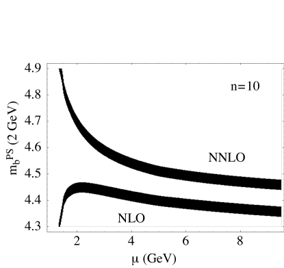
Figure 3: $m_{b}^{\rm PS}(2\,{\rm{GeV}})$, extracted from the $n=10$ moment in $\Upsilon$ sum rules at NLO (relative order $1/\sqrt{n}$) and NNLO (relative order $1/n$) as a function of renormalization scale $\mu$. (From Reference [93].) The dark region corresponds to the experimental uncertainty on the moment.

As shown in the figure, the NNLO corrections shift $m_{b}^{\rm PS}$ by about 250 MeV compared with the NLO result for a renormalization scale $\mu\sim 2\,{\rm{GeV}}$. This is about the same size as the shift in $m_{b}$ from LO to NLO, so perturbation theory does not appear to be converging well. Beneke & Signer [93] trace this behavior to the corresponding poor convergence of perturbation theory for the leptonic width of the $\Upsilon(1S)$, which dominates the sum rules for large $n$.

Given this poor behavior, it is difficult to estimate the theoretical error in $m_{b}$ reliably. A conservative approach would be to vary the renormalization scale $\mu$ between $m_{b}/2\sqrt{n}\sim 1.5\,{\rm{GeV}}$ and $2m_{b}/\sqrt{n}\sim 6\,{\rm{GeV}}$ and determine the error from the difference between the NLO and NNLO calculations. As Figure 3 shows, this corresponds to a variation in $m_{b}^{\rm PS}$ from $\sim 4.38$ to $\sim 4.84$ GeV, or about a $\pm 230\,{\rm{MeV}}$ uncertainty. Beneke & Signer [93] argue that, because the calculation becomes unstable below $\mu\sim 2\,{\rm{GeV}}$, it is more appropriate to determine the uncertainty from the variation in the NNLO result alone when $\mu$ is varied over the range $2\,{\rm{GeV}}<\mu<6\,{\rm{GeV}}$, which yields their quoted scale uncertainty of $\pm 100\,{\rm{MeV}}$.

Melnikov & Yelkhovsky [107] and Hoang [105, 106, 64] find similar behavior for perturbation theory for individual moments but have different ways of reducing the theoretical error. Melnikov & Yelkhovsky [107] interpret the first two terms in the nonrelativistic expansion as the first two terms of an alternating series. This can be converted via an Euler transformation to a more convergent series, from which they extract a smaller uncertainty. [However, these authors use larger moments, $n=14$–18, whose reliability has been questioned [105, 93].] It is difficult to prove that this rearrangement of the perturbative series is valid beyond the order at which it is currently calculated. In the absence of a more rigorous theoretical argument, it is not clear that the corresponding theoretical uncertainty is reduced by this procedure. In another approach, Hoang [105, 106, 64] notes that the behavior of the nonrelativistic expansion is much improved when one performs simultaneous fits to multiple moments from $n=4$ to $n=10$. This improves the stability of the fit greatly; both the shift in $m_{b}$ from NLO to NNLO and the renormalization-scale dependence of the result are much smaller than for single moments, which accounts for the smaller theoretical uncertainty quoted in these results. However, the reason for this improved behavior is not immediately clear, and the resulting theoretical error estimate depends on the correlations between the different experimental uncertainties in the masses and widths of the low-lying resonances. Once again, it is difficult to prove that this approach really gives a better-behaved perturbation series.

A poorly converging perturbative expansion frequently indicates that a parametrically large class of terms has not been resummed. The situation is similar to the calculation of the production cross section $\sigma(e^{+}e^{-}\to t\bar{t}X)$ near threshold, where the analogous calculation has been performed to NNLO (for a recent review, see Reference [112]). As with the $b{\bar{b}}$ sum rules, the NNLO correction to the cross section is roughly the same size as the NLO correction, and there is a large renormalization scale uncertainty in the NNLO result. It was shown for $t\bar{t}$ production that perturbation theory is much improved by the use of the renormalization group in NRQCD to sum logarithms of the form $\alpha_{s}^{m}\log^{m}v$ [33, 113]. For $b{\bar{b}}$ sum rules, the analogous renormalization-group–equation (RGE) calculation would sum terms of order $\alpha_{s}^{m}\log^{m}n$; it would be interesting to see if this gives a similar improvement.

In the absence of such a calculation, the poor behavior of perturbation theory suggests that the theoretical situation is not as stable as the values in Table 1 suggest. Given these issues, it is probably prudent to assign a conservative theoretical error to these determinations, at least until the poor convergence of perturbation theory is better understood.

Finally, Kühn & Steinhauser (109) avoid the issue of resumming Coulomb corrections by considering low moments ($n\leq 4$) for which fixed order perturbation theory is appropriate. As noted earlier, for such low moments the extracted value of $m_{b}$ is sensitive to $R(s)$ in the continuum regime where it is poorly measured. The authors replace the experimental measurement of $R(s)$ above the resonance region ($\sqrt{s}>11.2\,{\rm{GeV}}$) with its QCD prediction. This greatly reduces the uncertainty of $m_{b}$ since the perturbatively estimated uncertainty on the QCD prediction of $R(s)$ close to threshold is significantly smaller than the experimental uncertainty. The authors find

$$\overline{m}_{b}(\overline{m}_{b})=4.21\pm 0.05\,{\rm{GeV}}$$ (95)

which is consistent with the determinations from higher moments. However, unlike the determinations from higher moments, the uncertainty in this result depends strongly on the assumption that the QCD prediction for $R(s)$ (with perturbatively estimated errors) is valid very close to threshold, where it has not been well measured.

4.2 The $B$ System

Unlike the $b{\bar{b}}$ system, the $B$ system does not become perturbative in the heavy-quark limit, since the size of the hadron is still determined by nonperturbative physics. Hence, lattice QCD is best suited for determinations of $m_{b}$ from the $B$-meson spectrum. On the other hand, as discussed in Section 2, inclusive quantities such as the $B$-meson semileptonic width are dominated by short-distance ($r\sim 1/m_{b}$) physics, and are therefore sensitive to $m_{b}$ and perturbatively calculable in the heavy quark limit. Power corrections to the heavy-quark limit that scale like $(\Lambda_{\rm QCD}/m_{b})^{n}$ may be parameterized in the framework of HQET, allowing a precision determination of $m_{b}$.

Below we discuss determinations of $m_{b}$ from the $B$-meson spectrum and from inclusive $B$ decays. Typically, results in the $B$ system are quoted for $\bar{\Lambda}$ and $\lambda_{1}$ rather than a better-defined threshold mass. Because $\bar{\Lambda}$ is only defined order by order in perturbation theory, it is important to work consistently in $\alpha_{s}$. In this section, we therefore distinguish $\bar{\Lambda}$ extracted at one and two loops.

4.2.1 Lattice Calculations of the $B$-meson Spectrum

The best determination of the $b$-quark mass from lattice QCD calculations of the $B$-meson spectrum comes from calculations of the binding energy in the static limit, because the static self energy is known at three-loop order.

At present, there are two independent determinations of the $b$-quark mass from the static binding energy. The first one uses the results from numerical calculations of the $B$-meson system using static $b$ quarks [114, 115]. Allton et al. [114] use an $O(a)$ (tree-level) improved action for the light valence quarks. They perform their calculations at several lattice spacings and use the quenched approximation ($n_{f}=0$). Giménez et al. [115] obtain their results from numerical simulations with $n_{f}=2$ light Wilson quarks. Based on the numerical results of References [114] and [115], the authors of References [79, 116], and [115] obtain:

$$\overline{m}_{b}(\overline{m}_{b},n_{f}=0) = (4.30\pm 0.05\pm 0.05)\,{\rm{GeV}}$$ (96)

$$\overline{m}_{b}(\overline{m}_{b},n_{f}=2) = (4.26\pm 0.06\pm 0.07)\,{\rm{GeV}}\;.$$ (97)

The first error in Equation 96 is dominated by the uncertainty in the lattice spacing but also contains the statistical error of the numerical simulation and the effect of the uncertainty in $\alpha_{s}$. The second error in Equation 96 is the perturbative error in both Equation 3.2 and Equation 66. Similarly, the first error in Equation 97 is due to statistical and other systematic lattice errors, while the second error is the perturbative error. Because the $n_{f}$ dependence of the three-loop term in Equation 66 is unknown, at present, this error is larger than in the quenched case.

The second determination [117] uses the numerical results of References [118] and [119], which present numerical calculations of the $B$-meson spectrum using lattice NRQCD for the $b$ quark and an $O(a)$ improved action for the valence light quarks. The results of Reference [118] are obtained in the quenched approximation, whereas the results of Reference [119] come from numerical simulations with $n_{f}=2$ staggered sea quarks. After extrapolating the results of Reference [118] to the static limit, Collins [117] obtains a $b$-quark mass of

$$\overline{m}_{b}(\overline{m}_{b},n_{f}=0)=(4.34\pm 0.04\pm 0.05)\,{\rm{GeV}}\;.$$ (98)

The first error combines the statistical uncertainty with the uncertainty in the lattice spacing, and an estimate of residual discretization effects of $O(a^{2}\Lambda_{\rm QCD}^{2})$. The second error is the perturbative uncertainty. Collins [117] estimates that the inclusion of sea quarks lowers $\overline{m}_{b}$ by about $70\,{\rm{MeV}}$, having used two-loop perturbation theory to compare $\overline{m}_{b}(\overline{m}_{b},n_{f}=2)$ with $\overline{m}_{b}(\overline{m}_{b},n_{f}=0)$.

Both determinations use preliminary results for the coefficient of $\alpha_{P}^{3}$ in Equation 66, which have a larger uncertainty than the final result shown in Equation 66. Hence, the perturbative uncertainties given in Equation 96 and Equation 98 are slightly overestimated. In both determinations, a mild residual lattice-spacing dependence was observed, which is roughly equal to the statistical uncertainty, 10–30 MeV. Hence, in order to resolve the residual lattice-spacing dependence, the statistical accuracy of the numerical simulations must improve. This should be feasible with currently available computational resources. The error due to using the static limit is $O(\Lambda_{\rm QCD}/m_{b}$), and affects $\overline{m}_{b}$ at the $\sim 1\%$ level. This error will be removed when two- and three-loop results for the heavy-quark self energy at finite quark mass become available. The $n_{f}$ dependence is similar in size to the perturbative uncertainty. Numerical simulations with $n_{f}=3$ sea quarks are needed to bring this error completely under control.

Heitger & Sommer suggest a new method for determining the $b$-quark mass based on the nonpertubative methods developed by the ALPHA collaboration [120]. The authors obtain a preliminary result for $\overline{m}_{b}(4\,{\rm{GeV}})$ in the quenched approximation, which corresponds to $\overline{m}_{b}(\overline{m}_{b})=4.48\pm 0.13\,{\rm{GeV}}$ [121]. Error analysis is in progress.

As discussed in Section 3.4, the determination of the binding energy ${\cal E}$ away from the static limit can be used to extract both ${\bar{\Lambda}}$ and $\lambda_{1}$ by fitting the binding energy to Equation 67. Kronfeld & Simone [85] used results of numerical simulations of the $B$-meson system (as obtained in References [122, 123, 124]) to determine these parameters. They find

$${\bar{\Lambda}}=0.68^{+0.02}_{-0.12}\,{\rm{GeV}}$$ (99)

and

$$\lambda_{1}=-(0.45\pm 0.12)\,{\rm{GeV}}^{2},$$ (100)

where the error includes statistical and lattice-spacing errors. These results come from numerical simulations that were performed in the quenched approximation, for which no solid error analysis exists at present. The results are based on one-loop perturbation theory, in which the coupling is evaluated at the scale $q^{*}\sim 1/a$, determined from Equation 74 (which is similar to the BLM scale). The errors in Equations 99–100 do not include an estimate of the perturbative uncertainty. Earlier determinations of ${\bar{\Lambda}}$ and $\lambda_{1}$ were based on numerical simulations of lattice HQET [125].

4.2.2 QCD Sum Rules

The first QCD-based determinations of $m_{b}$ from the $B$ system relied on the QCD sum rules of Shifman, Vainshtein & Zakharov (SVZ) [91]. In this approach, correlators of hadronic currents are studied at intermediate distances (of order $\sim 1\,{\rm{GeV}}^{-1}$). At this energy scale, one can either expand the product of currents in an OPE as a sum of local operators, or evaluate the currents by inserting complete sets of states between the operators. For sufficiently small separation, the OPE is dominated by the lowest-dimension operators; for sufficiently large separation, the sum over intermediate states is dominated by the lowest-lying hadronic states. QCD sum rules rely on a “window” of distance scales for which both approaches hold (in practice, the convergence is improved by the use of Borel transforms, and the window is in the Borel parameter), and use local duality to model the contributions of all but the lowest-lying states with the perturbative QCD prediction. In this way, local duality is used to relate hadronic matrix elements (from the sum over states) to a small number of condensates (from the OPE).

QCD sum rules have been remarkably successful at describing many low-energy features of QCD and have been used extensively to study properties of heavy quarks, including $m_{b}$ [126, 127, 128, 129] (for reviews of recent results, see Reference [130]). Because of their well-defined heavy-quark limit, QCD sum rules may be used to determine the parameters of HQET. However, unlike the other approaches discussed in this article, they are not strictly model-independent; it is difficult to quantify the systematic errors inherent in the assumption of local duality in the intermediate window. As a result, the sum rules cannot be consistently improved by calculating higher-order corrections.

With this caveat in mind, the HQET sum rule determination of ${\bar{\Lambda}}$ gives [128, 129]

$${\bar{\Lambda}}\,\mbox{(1\ loop)}=\cases{\displaystyle 400-600\,{\rm{MeV}}&Reference \cite[cite]{[\@@bibref{}{bbbd92}{}{}]}\cr\displaystyle 570\pm 70\,{\rm{MeV}}&Reference \cite[cite]{[\@@bibref{}{neub92}{}{}]}\cr}$$ (101)

The sum rule for $\lambda_{1}$ is more problematic. Two calculations report conflicting results: $\lambda_{1}=-0.5\pm 0.2\,{\rm{GeV}}^{2}$ [131] and $\lambda_{1}=-0.1\pm 0.05\,{\rm{GeV}}^{2}$ [132]. The discrepancy has been traced to the the contribution of an off-diagonal matrix element involving an excited pseudoscalar $B$ meson [69], but it is currently unresolved.

Several extractions do not explicitly use the heavy-quark limit. From the sum rules for the pseudoscalar two-point function, Narison [127] obtains the two-loop result

$$m_{b}=4.59\pm 0.06\,{\rm{GeV}}\Rightarrow\overline{m}_{b}=4.05\pm 0.06\,{\rm{GeV}},$$ (102)

where the errors do not address the assumptions inherent in the sum rules.

4.2.3 Inclusive Moments

As discussed in Section 2, inclusive differential decay rates of heavy hadrons may be used to determine $m_{b}$ without the additional assumptions required by QCD sum rules. The first attempts to extract HQET parameters from inclusive decays combined the rates for $B\to X_{c}e(\mu)\bar{\nu}_{e(\mu)}$ and $D\to X_{u,s}\ell\bar{\nu}_{\ell}$ decay [133, 134] as well as $B\to X_{c}\tau\bar{\nu}_{\tau}$ [135], but these extractions rely on the validity of the heavy-quark expansion for inclusive charm decays. As a result, they have large errors.

With the advent of precision measurements in recent years, direct determinations of $\bar{\Lambda}$ and $\lambda_{1}$ may be made purely in the $B$ system. Of the infinite number of inclusive quantities, we focus on three that have been widely used to determine $m_{b}$: the shape of the charged-lepton energy spectrum in $B\to X_{c}\ell\bar{\nu}_{\ell}$, moments of the hadronic invariant mass spectrum in $B\to X_{c}\ell\bar{\nu}_{\ell}$, and moments of the photon spectrum in $B\to X_{s}\gamma$. Power corrections to these quantities are all known to $O(1/m_{b}^{3})$, and the one-loop perturbative corrections are also known. In addition, the $O(\alpha_{s}^{2}\beta_{0})$ (BLM) piece of the two-loop term, which is expected to dominate the two-loop result, is known for most of these observables. Since there are more free parameters at $O(1/m_{b}^{3})$ than current data can constrain, estimates of the sizes of these terms are typically used to estimate the theoretical uncertainty in the extraction of ${\bar{\Lambda}}$ and $\lambda_{1}$ from a given observable.

For consistency in comparing different approaches, the estimating technique proposed in Reference [136] is often used. In this approach, the parameters at $O(1/m_{b}^{3})$ are independently varied over a range of $\pm(500\,{\rm{MeV}})^{3}$ and the region containing 68% of the points in the ${\bar{\Lambda}},\ \lambda_{1}$ plane is taken as an indication of the theoretical error. This approach allows the relative theoretical errors from different observables to be compared in a consistent way, but the arbitrariness of this procedure should be kept in mind when interpreting the experimental results. Changing the range of variation of the parameters to, for example, $\pm 600\,{\rm{MeV}}$ would increase the theoretical error by $\sim 70\%$. Figure 4 compares the relative theoretical uncertainties in the $(\bar{\Lambda},\lambda_{1})$ plane obtained by this technique from hypothetical measurements of moments of the charged-lepton energy spectrum, hadronic invariant mass, and photon energy spectrum in $B\to X_{s}\gamma$, discussed in the following sections.

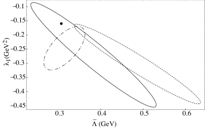
Figure 4: Relative theoretical uncertainties in $\bar{\Lambda}$ and $\lambda_{1}$ from ($a$) the lepton energy spectrum in semileptonic $B$ decay (solid line), ($b$) the hadronic invariant mass spectrum in semileptonic $B$ decay (dashed line), and ($c$) the $B\to X_{s}\gamma$ photon spectrum (dashed-dotted line), from References [137] and [138].

In addition to the experimental determinations of $\bar{\Lambda}$ and $\lambda_{1}$, it is possible to derive purely theoretical constraints. By using sum rules that relate exclusive decay form factors to $\lambda_{1}$ and $\lambda_{2}$ and demanding that the exclusive rate be less than the inclusive rate, Bigi et al. [68] derived the constraint

$$-\lambda_{1}>3\lambda_{2}\simeq 0.36\,{\rm{GeV}}^{2}+\dots,$$ (103)

where the ellipses denote radiative corrections. The authors [68] use a definition of $\lambda_{1}(\mu)$ in which the matrix element in Equation 2.1 has been defined with a cutoff $\mu$, as discussed in Section 3.3.1. This differs from the definition of $\lambda_{1}$ in dimensional regularization, and the radiative corrections to the bound of Equation 103 differ in the two schemes. Equation 103 in the ${\overline{\mbox{MS}}}$ scheme is considerably weakened by radiative corrections [139]; the best bound quoted is $-\lambda_{1}>0.01\,{\rm{GeV}}^{2}$, and the two-loop corrections were large enough to challenge the validity of perturbation theory. The radiative corrections to the bound on $\lambda_{1}(\mu)$ for $\mu\sim 1\,{\rm{GeV}}$ are expected to be better behaved [69].

The difference between the two schemes is formally higher-order than the expressions we consider in this section. Within experimental errors, the bound in Equation 103 appears to be satisfied.

The Charged-Lepton Energy Spectrum:

Moments of the charged-lepton energy spectrum of the form

$$M^{(n)}_{\ell}=\int_{0}^{E_{\ell}^{\rm max}}E_{\ell}^{n}{d\Gamma\over dE_{\ell}}dE_{\ell}$$ (104)

were suggested [140] as a sensitive probe of the mass difference $m_{b}-m_{c}$. However, because of the large background from secondary leptons (for example, from charm decays), it is difficult to measure the charged-lepton spectrum over the full kinematic range. [CLEO [141] imposed a cut $E_{\ell}>1.4\,{\rm{GeV}}$, and modeled the spectrum at lower energies.] To avoid the model dependence of the low-$E_{\ell}$ region, Gremm et al. [142] proposed the following observables:

$$R_{1}\equiv{\displaystyle{\int_{1.5\,{\rm{GeV}}}^{E_{\ell}^{\rm max}}E_{\ell}{d\Gamma\over dE_{\ell}}dE_{\ell}}\over\displaystyle{\int_{1.5\,{\rm{GeV}}}^{E_{\ell}^{\rm max}}{d\Gamma\over dE_{\ell}}dE_{\ell}}},\ R_{2}\equiv{\displaystyle{\int_{1.7\,{\rm{GeV}}}^{E_{\ell}^{\rm max}}{d\Gamma\over dE_{\ell}}dE_{\ell}}\over\displaystyle{\int_{1.5\,{\rm{GeV}}}^{E_{\ell}^{\rm max}}{d\Gamma\over dE_{\ell}}dE_{\ell}}}\;.$$ (105)

Gremm and colleagues calculated expressions for $R_{1}$ and $R_{2}$ to $O(1/m_{b}^{2})$ and $O(\alpha_{s})$ [142], and calculated the $O(1/m_{b}^{3})$ corrections [136] and the $O(\alpha_{s}^{2}\beta_{0})$ terms [143]. A correction due to the boost of the leptons must also be taken into account [142]. $R_{1}$ and $R_{2}$ constrain similar linear combinations of ${\bar{\Lambda}}$ and $\lambda_{1}$, so the corresponding solid ellipse in Figure 4 constrains one linear combination much better than ${\bar{\Lambda}}$ or $\lambda_{1}$ individually.

The Hadronic Invariant Mass Spectrum:

Moments of the form

$$\langle(s_{H}-{\overline{m}_{D}}^{2})^{n}\rangle={1\over\Gamma}\int_{0}^{m_{B}^{2}}(s_{H}-{\overline{m}_{D}}^{2})^{n}{d\Gamma\over ds_{H}}ds_{H},$$ (106)

where $s_{H}$ is the invariant mass of the final-state hadrons and $\overline{m}_{D}=(m_{D}+3m_{D}^{*})/4$ is the spin-averaged meson mass, have been proposed [59]. At the parton level, the invariant mass $s_{H}$ of the final hadronic state in semileptonic $b\to c$ decay is fixed at $m_{c}^{2}$, so positive moments of $s_{H}-\overline{m}_{D}^{2}$ only get contributions in the OPE at $O(\alpha_{s})$ and $O(1/m_{b})$, making them a good probe of the power corrections in the OPE. Falk et al. calculated expressions for the first two moments, $\langle(s_{H}-\overline{m}_{D}^{2})\rangle$ and $\langle(s_{H}-\overline{m}_{D}^{2})^{2}\rangle$ [59], to $O(1/m_{b}^{2})$ and $\alpha_{s}^{2}\beta_{0}$, while Gremm & Kapustin calculated the $O(1/m_{b}^{3})$ terms [136].

Falk et al. [59] used the experimentally measured branching fraction to the excited states $D_{1}$ and $D_{2}^{*}$ to put lower bounds on the first two moments, excluding a region of the ${\bar{\Lambda}}-\lambda_{1}$ plane. The early DELPHI result of $34\pm 7\%$ semileptonic branching fraction to these states gives a strong bound of $\bar{\Lambda}>410\,{\rm{MeV}}$, but later measurements that put this branching fraction closer to 11% weaken this bound considerably, to $\bar{\Lambda}\mathrel{\mathchoice{\lower 3.0pt\vbox{\halign{\\$\displaystyle\hfill#\hfil\\$\cr $\displaystyle\hfill>\hfil\\ \crcr $\displaystyle\hfill\sim\hfil\\ \crcr}}}{\lower 3.0pt\vbox{\halign{\\$\textstyle\hfill#\hfil\\$\cr $\textstyle\hfill>\hfil\\ \crcr $\textstyle\hfill\sim\hfil\\ \crcr}}}{\lower 3.0pt\vbox{\halign{\\$\scriptstyle\hfill#\hfil\\$\cr $\scriptstyle\hfill>\hfil\\ \crcr $\scriptstyle\hfill\sim\hfil\\ \crcr}}}{\lower 3.0pt\vbox{\halign{\\$\scriptscriptstyle\hfill#\hfil\\$\cr $\scriptscriptstyle\hfill>\hfil\\ \crcr $\scriptscriptstyle\hfill\sim\hfil\\ \crcr}}}}100\,{\rm{MeV}}$. More useful is the direct measurement of these moments by the CLEO collaboration, made possible by reconstructing the missing neutrino. This introduces a subtlety because the technique of neutrino reconstruction requires placing a lower cut of $1.5\,{\rm{GeV}}$ on the charged-lepton energy; Reference [137] presents the complete theoretical prediction, including the effects of the lepton cut.

The first moment of the invariant mass spectrum constrains roughly the same linear combination of ${\bar{\Lambda}}$ and $\lambda_{1}$ as $R_{1}$ and $R_{2}$, discussed above. The second moment constrains a roughly orthogonal linear combination, but the theoretical prediction is very uncertain because of the effects of $O(1/m_{b}^{3})$ terms in the OPE, so the dashed ellipse in Figure 4 usefully constrains only the same rough linear combination of parameters as $R_{1}$ and $R_{2}$.

The $B\to X_{s}\gamma$ Photon Spectrum:

Comparison of the measured weak radiative $B\to X_{s}\gamma$ decay rate with theory is an important test of the standard model. In contrast to the decay rate itself, the shape of the photon spectrum is not expected to be sensitive to new physics [144, 145] but instead serves as an additional inclusive quantity that may be used to determine ${\bar{\Lambda}}$ and $\lambda_{1}$.

The photon spectrum in the large-energy region ($E_{\gamma}\mathrel{\mathchoice{\lower 3.0pt\vbox{\halign{\\$\displaystyle\hfill#\hfil\\$\cr $\displaystyle\hfill>\hfil\\ \crcr $\displaystyle\hfill\sim\hfil\\ \crcr}}}{\lower 3.0pt\vbox{\halign{\\$\textstyle\hfill#\hfil\\$\cr $\textstyle\hfill>\hfil\\ \crcr $\textstyle\hfill\sim\hfil\\ \crcr}}}{\lower 3.0pt\vbox{\halign{\\$\scriptstyle\hfill#\hfil\\$\cr $\scriptstyle\hfill>\hfil\\ \crcr $\scriptstyle\hfill\sim\hfil\\ \crcr}}}{\lower 3.0pt\vbox{\halign{\\$\scriptscriptstyle\hfill#\hfil\\$\cr $\scriptscriptstyle\hfill>\hfil\\ \crcr $\scriptscriptstyle\hfill\sim\hfil\\ \crcr}}}}1.5\,{\rm{GeV}}$) is dominated by the operator

$$O_{7}=\displaystyle{e\over 16\pi^{2}}\,m_{b}\bar{s}_{L\alpha}\sigma^{\mu\nu}b_{R\alpha}F_{\mu\nu},$$ (107)

with small contributions from four-fermion operators. For lower photon energies there is a large background from nonleptonic decays, so it is necessary to restrict measurements to large photon energies. Kapustin & Ligeti [144] studied moments of the form

$$M^{(n)}_{\gamma}(E_{0})={\displaystyle{\int_{E_{0}}^{E_{\gamma}^{\rm max}}E_{\gamma}^{n}{d\Gamma\over dE\gamma}dE_{\gamma}}\over\displaystyle{\int_{E_{0}}^{E_{\gamma}^{\rm max}}{d\Gamma\over dE\gamma}dE_{\gamma}}}.$$ (108)

At tree level, measurements of the first moment and variance of the photon energy directly determine $\bar{\Lambda}$ and $\lambda_{1}$, respectively:

$$M^{(1)}_{\gamma}(E_{0}) = {m_{B}-{\bar{\Lambda}}\over 2}\left[1+\delta m_{1}\left({2E_{0}\over m_{b}}\right)+\dots\right],$$ (109)

$$M^{(2)}_{\gamma}(E_{0})-(M^{(1)}_{\gamma}(E_{0}))^{2} = -{\lambda_{1}\over 12}+\left({m_{b}\over 2}\right)^{2}\left[\delta m_{2}\left({2E_{0}\over m_{b}}\right)-2\delta m_{1}\left({2E_{0}\over m_{b}}\right)+\dots\right],$$

where $\delta m_{1}$ and $\delta m_{2}$ are perturbative corrections, and the ellipses denote terms of order $\alpha_{s}^{2}$, $\alpha_{s}\Lambda_{\rm QCD}^{2}/m_{b}^{2}$, and $\Lambda_{\rm QCD}^{3}/m_{b}^{3}$.

Corrections to these results of order $\alpha_{s}^{2}\beta_{0}$ [146] and $(\Lambda_{\rm QCD}/m_{b})^{3}$ [138] have been calculated, and the estimated theoretical error is shown as the dot-dashed line in Figure 4. An important additional uncertainty in these results arises from the effects of the photon cut $E_{0}$. Only moments of the photon spectrum are calculable in the OPE; the precise shape is determined by the nonperturbative parton distribution function of the $b$ quark [147] and so the effects of the cut must be modeled. Simple models for the distribution function suggest that a photon cut of $E_{0}\mathrel{\mathchoice{\lower 3.0pt\vbox{\halign{\\$\displaystyle\hfill#\hfil\\$\cr $\displaystyle\hfill<\hfil\\ \crcr $\displaystyle\hfill\sim\hfil\\ \crcr}}}{\lower 3.0pt\vbox{\halign{\\$\textstyle\hfill#\hfil\\$\cr $\textstyle\hfill<\hfil\\ \crcr $\textstyle\hfill\sim\hfil\\ \crcr}}}{\lower 3.0pt\vbox{\halign{\\$\scriptstyle\hfill#\hfil\\$\cr $\scriptstyle\hfill<\hfil\\ \crcr $\scriptstyle\hfill\sim\hfil\\ \crcr}}}{\lower 3.0pt\vbox{\halign{\\$\scriptscriptstyle\hfill#\hfil\\$\cr $\scriptscriptstyle\hfill<\hfil\\ \crcr $\scriptscriptstyle\hfill\sim\hfil\\ \crcr}}}}2\,{\rm{GeV}}$ is sufficient for the dominant uncertainty in ${\bar{\Lambda}}$ to be set by the $1/m_{b}^{3}$ terms, whereas the corresponding uncertainty in $\lambda_{1}$ is very model-dependent [138, 145]. Hence, only ${\bar{\Lambda}}$ is likely to be determined accurately by the photon spectrum.

Experimental Results:

From CLEO measurements (tabulated in Reference [148]), Gremm et al. [142] determined the experimental values of $R_{1}$ and $R_{2}$,

$$R_{1}^{\rm{exp}}=1.7831\,{\rm{GeV}},\ \ R_{2}^{\rm{exp}}=0.6159,$$ (110)

which lead to the values

$${\bar{\Lambda}}(1\ \mbox{loop})=0.39\pm 0.11\,{\rm{GeV}},\ \lambda_{1}=-0.19\pm 0.10\,{\rm{GeV}}^{2},$$ (111)

where the uncertainty corresponds to the experimental $1\sigma$ statistical error. The estimated uncertainty due to $O(1/m_{b}^{3})$ terms is larger than this [136]. The $O(\alpha_{s}^{2}\beta_{0})$ terms calculated in Reference [143] shift the central values slightly,

$${\bar{\Lambda}}(2\ \mbox{loop})=0.33\ {\rm{GeV}},\ \lambda_{1}=-0.17\ {\rm{GeV}}^{2}.$$ (112)

More recently, $R_{1}$ and $R_{2}$ were calculated in the 1S scheme by Bauer & Trott [149]. Using the values in Equation 109, they find

$$\bar{\Lambda}_{1S}=0.47\pm 0.10_{\rm E}\pm 0.08_{\rm T}\,{\rm{GeV}},\ \ \lambda_{1}=-0.16\pm 0.11_{E}\pm 0.08_{T}\,{\rm{GeV}}^{2},$$ (113)

where $\bar{\Lambda}_{1S}\equiv m_{B}-m_{b}^{1S}$, corresponding to $m_{b}^{1S}=4.84\pm 0.10_{E}\pm 0.08_{T}$. This gives the ${\overline{\mbox{MS}}}$ mass

$$\overline{m}_{b}=4.31\pm 0.13\,{\rm{GeV}},$$ (114)

adding the experimental and theoretical errors in quadrature. The CLEO collaboration [150] has recently measured these moments, and a preliminary analysis gives, for decays to electrons, $R_{1}=1.7797\pm 0.0007_{\rm stat}\pm 0.0007_{\rm sys}$ and $R_{2}=0.6173\pm 0.0016_{\rm stat}\pm 0.0014_{\rm sys}$ (with compatible results for muons). This in turn gives $m_{b}^{1S}=4.81\pm 0.09_{\rm E}$ (electrons) and $m_{b}^{1S}=4.87\pm 0.11_{\rm E}$ (muons), where only the experimental error is quoted.

In 1998, the CLEO collaboration published preliminary measurements of the first and second hadronic invariant mass moments, as well as the first two lepton-energy moments $M_{\ell}^{(1)}$ and $M_{\ell}^{(2)}$ [151]. The values of $\bar{\Lambda}$ and $\lambda_{1}$ obtained from the hadronic invariant mass moments differed from the values obtained from the lepton-energy moments, although the discrepancy was only at the $\sim 2\sigma$ level. Two possible issues are the use of the second hadronic invariant mass moment, which is not theoretically well-controlled [137], and the model-dependent extrapolation of the data into the region $E_{\ell}\leq 0.6\,{\rm{GeV}}$ [152].

More recently, two new published CLEO measurements of the hadronic invariant mass and photon energy spectra [153, 154] give

$$\langle s_{H}-\overline{m}_{D}^{2}\rangle = 0.251\pm 0.023\pm 0.062\ {\rm{GeV}}^{2}$$

$$\langle(s_{H}-\overline{m}_{D}^{2})^{2}\rangle = 0.639\pm 0.056\pm 0.178\ {\rm{GeV}}^{4}$$ (115)

and

$$\langle E_{\gamma}\rangle = 2.346\pm 0.032\pm 0.011\ {\rm{GeV}}$$

$$\langle\left(E_{\gamma}-\langle E_{\gamma}\rangle\right)^{2}\rangle = 0.0226\pm 0.0066\pm 0.0020\ {\rm{GeV}}^{2}.$$ (116)

Note that the photon spectrum was measured only down to $E_{\gamma}=2.0\,{\rm{GeV}}$, and the moments fitted to theoretical predictions that included the photon-energy cut [146]. Because of the theoretical uncertainties discussed above for the second moments, robust constraints are obtained only from the two lowest moments (Figure 5).

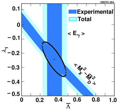
Figure 5: Determination of $\bar{\Lambda}$ and $\lambda_{1}$ from the hadronic energy spectrum and photon spectrum in semileptonic and radiative $B$ decays, from Reference [153].

This leads to the values

$${\bar{\Lambda}}\ \mbox{(two\ loop)} = 0.35\pm 0.07_{E}\pm 0.10_{T}\ {\rm{GeV}}$$

$$\lambda_{1} = -0.236\pm 0.071_{E}\pm 0.078_{T}\ {\rm{GeV}}^{2}$$ (117)

(where the theoretical error includes an estimate of the $1/m_{b}^{3}$ operators as well as the scale dependence of $\alpha_{s}$), in good agreement with Equation 112.

As we have discussed, it is difficult to assign a perturbative error to the extraction of $\bar{\Lambda}$ because of its inherent ambiguity; it is better to work with a well-defined threshold mass. For the $1S$ mass, this gives (see also Reference [155])

$$m_{b}^{1S}=4.75\pm 0.07_{E}\,{\rm{GeV}}$$ (118)

corresponding to

$$\overline{m}_{b}=4.22\pm 0.07_{E}\pm 0.05_{1/m^{3}}\,{\rm{GeV}}$$ (119)

where the first error is the experimental uncertainty and the second error is an estimate of the uncertainty due to $O(1/m_{b}^{3})$ corrections obtained from the width of the ellipse in Figure 4. This result is in good agreement with the results from the $\Upsilon$ system. The perturbative uncertainty is not included in the error, since it would require directly fitting the moments in the $1S$ scheme to the data, which has not yet been done. Nevertheless, the theoretical error appears comparable to the theoretical error from the $\Upsilon$ system, though the sources of theoretical uncertainty are completely different.

4.3 High-Energy Determinations

The DELPHI and ALEPH collaborations at LEP [156, 157] have analyzed $e^{+}e^{-}$ annihilation into heavy-quark jets, which depends on $m_{b}$. Using the NLO predictions [158], they find

$$\overline{m}_{b}(m_{Z}) = 2.67\pm 0.25_{\rm stat}\pm 0.34_{\rm had}\pm 0.27_{\rm thy}\,{\rm{GeV}}\ \ \ \rm{(DELPHI)}$$ (120)

$$\overline{m}_{b}(m_{Z}) = 3.27\pm 0.22_{\rm stat}\pm 0.22_{\rm exp}\pm 0.38_{\rm had}\pm 0.16_{\rm thy}\,{\rm{GeV}}\ \ \rm{(ALEPH)}$$

(where “had” denotes hadronization uncertainties). Although the precision is not comparable to that of low-energy determinations, this first measurement of $m_{b}$ away from threshold provides a statistically significant check of the running of $\overline{m}_{b}(\mu)$. Both results are in good agreement with the predicted QCD running of the low-energy masses determined from the $\Upsilon$ system. For example, running the DELPHI result down to $m_{b}$ gives

$$\overline{m}_{b}(\overline{m}_{b})=3.91\pm 0.67\,{\rm{GeV}},$$ (121)

in agreement with other determinations (but with significantly larger error).

5 CONCLUSIONS

All the precision determinations of $m_{b}$ discussed in this review are currently dominated by theoretical errors. Table 2 summarizes the model-independent extractions of $\overline{m}_{b}$ from the different approaches discussed in this paper. We assign conservative theoretical errors to the results, which encompass the ranges given in the literature.

Table 2: Summary of model-independent determinations of $\overline{m}_{b}(\overline{m}_{b})^{\rm a}$

System	Method (Section)	Caveat	$\overline{m}_{b}(\overline{m}_{b})\ ({\rm{GeV}})$
$\Upsilon$	$1S$ mass	nonperturbative terms	$4.23\pm 0.11$
	sum rules	poor convergence	$4.20\pm 0.10$
	lattice QCD	sea-quark effects	$4.26\pm 0.11$
$B$	Inclusive moments	$1/m_{b}^{3},\ {\rm duality}$
	(i) lepton spectrum		$4.31\pm 0.13$
	(ii) photon energy/		$4.22\pm 0.09\pm O(\alpha_{s}^{2})$
	hadron invt. mass
	lattice QCD (static limit)	sea-quark effects	$4.26\pm 0.09$
	OUR DETERMINATION		$4.24\pm 0.11$

^aThe error bars represent our estimate of the uncertainties, based on the discussion in Section 4. Theoretical and experimental uncertainties have been added in quadrature. The “Caveat” column identifies the most problematic aspect of the theory used in each determination, as discussed in the text. The last row gives our best determination of $\overline{m}_{b}(\overline{m}_{b})$, as discussed in the text.

The determination of $m_{b}$ from the perturbative calculation of the $\Upsilon(1S)$ mass is limited by our knowledge of the nonperturbative corrections. The associated error is difficult to estimate and to improve, since the corresponding OPE does not appear to converge well.

Sum rules for spectral moments of $b{\bar{b}}$ production are less sensitive to nonperturbative effects and have the potential to give very accurate determinations of $m_{b}$. The main issue in present determinations is the poorly behaved perturbative series, which might be improved via a renormalization-group resummation. In the absence of such a calculation, the perturbative uncertainty is difficult to estimate reliably.

The $m_{b}$ determination from inclusive $B$-meson decays is limited by nonperturbative effects at $O(\Lambda_{\rm QCD}^{3}/m_{b}^{3})$, which are estimated to be at the $\pm 50$–$70\,{\rm{MeV}}$ level for the moments we have discussed [although these may be smaller for other choices of moments [149]]. It may be possible to better constrain these terms from the fits to the different moments, or from lattice calculations. Additional uncertainty from violations of quark-hadron duality is also possible. This uncertainty is difficult to quantify but may be experimentally tested by demanding consistency between different moments. Converting the determination of $\bar{\Lambda}$ from the photon spectrum in $B\to X_{s}\gamma$ in Equation 116 to a threshold mass will allow the perturbative uncertainty to be accurately estimated, and perturbative corrections are expected to be well-behaved.

With the exception of the static result, determinations of $m_{b}$ from lattice QCD are presently limited by the low order at which the perturbative corrections are known. However, perturbative calculations of the two-loop corrections are currently in progress, and it may be possible to extract the three-loop corrections by using numerical techniques. Hence, we can expect a significant reduction of the perturbative uncertainty. In principle, this uncertainty can be reduced even further through the use of nonperturbative renormalization prescriptions. At present, all lattice calculations suffer from the incomplete inclusion of sea-quark effects, which is the most troublesome source of systematic error. However, this error appears to have only a small effect on the $b$-quark mass determinations. The results listed in Table 2 were obtained from numerical simulations with $n_{f}=2$ sea quarks. Given sufficient computational resources, all systematic errors that arise in lattice QCD calculations are in principle controllable and systematically reducible. Current progress in numerical simulations of sea-quark effects using improved actions [159] gives us reason to believe that lattice results with good control over all systematic errors may be achieved in the next few years.

To put these uncertainties into context, consider the precision in $m_{b}$ presently required for CKM physics. Probably the quantity most sensitive to $m_{b}$ is $|V_{ub}|$, as determined from the inclusive $B$-meson decay, $b\to u\ell\nu$. This rate is proportional to $m_{b}^{5}$. Hence, an uncertainty in $m_{b}$ of $\pm 100\,{\rm{MeV}}$ corresponds to a $\pm 12\%$ uncertainty in the total semileptonic $b\to u$ decay width, or a $\pm 6\%$ uncertainty in $|V_{ub}|$. In practice, the sensitivity of $|V_{ub}|$ to $m_{b}$ may be even stronger because of the experimental cuts necessary to reduce the $b\to c$ background. For example, in a recent proposal for determining $|V_{ub}|$ through a set of optimized kinematic cuts [160], the uncertainty in $m_{b}$ is the dominant source of theoretical error: a $\pm 80\,{\rm{MeV}}$ ($\pm 2\%$) uncertainty in $m_{b}$ results in a $\pm 15\%$ uncertainty in $|V_{ub}|$. Thus, for precision CKM physics, the error on $m_{b}$ should be reduced to less than $100\,{\rm{MeV}}$.

As Table 2 indicates, current determinations are approaching this level, and the different results agree very well with one another. Indeed, the variation of the central values given in Table 2 is smaller than the uncertainties associated with each determination. However, given the discussion above, we feel that it is inappropriate to reduce the error in the average. Hence, our best estimate of the $b$-quark mass is

$$\overline{m}_{b}(\overline{m}_{b})=4.24\pm 0.11\;{\rm{GeV}},$$ (122)

where the central value and uncertainty have been chosen to accommodate most of the spread in the theoretical determinations. If we run this result up to the $Z$-boson mass, we obtain

$$\overline{m}_{b}(m_{Z})=2.94\pm 0.09\;{\rm{GeV}}\,.$$ (123)

in good agreement with the high-energy determinations shown in Equation 117. Currently, determinations of $m_{b}$ from lattice QCD are comparable in accuracy to determinations from perturbative QCD, and the prospects for improving on the current accuracy of $m_{b}$ determinations from several of these methods over the next few years are excellent.

References

- [1] Buras AJ, et al. Nucl. Phys. B 135:66 (1978); Dimopoulos S, Hall LJ, Raby S. Phys. Rev. Lett. 68:1984 (1992)
- [2] Harrison PF, Quinn HR (BABAR Collab.). The BaBar Physics Book: Physics at an Asymmetric B Factory. SLAC-R-0504 (1998); Anikeev K, et al. B Physics at the Tevatron: Run II and Beyond, hep-ph/0201071
- [3] Buchalla G, Buras AJ. Nucl. Phys. B 548:309 (1999)
- [4] De Rujula A, Georgi H, Glashow SL. Phys. Rev. D 12:147 (1975); Isgur N, Karl G. Phys. Rev. D 18:4187 (1978)
- [5] Richardson JL. Phys. Lett. B82:272 (1979); Martin A. Phys. Lett. B93:338 (1980); Igi K, Ono S. Phys. Rev. D 33:3349 (1986)
- [6] Eichten E, et al. Phys. Rev. D 21:203 (1980)
- [7] Georgi H. Annu. Rev. Nucl. Part. Sci. 43:209 (1993); Kaplan DB. nucl-th/9506035; Manohar AV. hep-ph/9606222; Bedaque PF, van Kolck U. Annu. Rev. Nucl. Part. Sci. 52. In press (2002)
- [8] Shuryak EV. Phys. Lett. B93:134 (1980); Nussinov S, Wetzel W. Phys. Rev. D 36:130 (1987)
- [9] Shifman MA, Voloshin MB. Sov. J. Nucl. Phys. 45:292 (1987) [Yad. Fiz. 45:463 (1987)]; Sov. J. Nucl. Phys. 47:511 (1988) [Yad. Fiz. 47:801 (1988)]
- [10] Politzer HD, Wise MB. Phys. Lett. B206:681 (1988); Phys. Lett. B208:504 (1988)
- [11] Isgur N, Wise MB. Phys. Lett. B232:113 (1989); Phys. Lett. B237:527 (1990)
- [12] Eichten E, Hill B. Phys. Lett. B234:511 (1990)
- [13] Georgi H. Phys. Lett. B240:447 (1990)
- [14] Manohar AV, Wise MB. Heavy Quark Physics. Cambridge, UK: Cambridge Univ. Press (2000); Manohar AV, Wise MB, Neubert M. Phys. Rep. 245:259 (1994); Shifman MA. hep-ph/9510377; Falk AF. hep-ph/0007339
- [15] Falk AF, Neubert M, Luke ME. Nucl. Phys. B 388:363 (1992)
- [16] Luke ME, Manohar AV. Phys. Lett. B286:348 (1992)
- [17] Czarnecki A, Grozin AG. Phys. Lett. B405:142 (1997)
- [18] Eichten E, Hill B. Phys. Lett. B243:427 (1990); Falk AF, Grinstein B, Luke ME. Nucl. Phys. B 357:185 (1991)
- [19] Poggio EC, Quinn HR, Weinberg S. Phys. Rev. D 13:1958 (1976)
- [20] Braaten E, Narison S, Pich A. Nucl. Phys. B 373:581 (1992)
- [21] Chay J, Georgi H, Grinstein B. Phys. Lett. B247:399 (1990)
- [22] Bigi II, Uraltsev NG, Vainshtein AI. Phys. Lett. B293:430 (1992); erratum, Phys. Lett. B297:477 (1992); Bigi II, et al. Phys. Rev. Lett. 71:496 (1993)
- [23] Manohar AV, Wise MB. Phys. Rev. D 49:1310 (1994)
- [24] Blok B, et al. Phys. Rev. D 49:3356 (1994); Erratum, Phys. Rev. D 50:3572 (1994)
- [25] Isgur N. Phys. Lett. B448:111 (1999)
- [26] Shifman MA. Mod. Phys. Lett. A10:605 (1995)
- [27] Bigi II, et al. Phys. Rev. D 59:054011 (1999); Grinstein B, Lebed RF. Phys. Rev. D 57:1366 (1998); Lebed RF, Uraltsev NG. Phys. Rev. D 62:094011 (2000)
- [28] Bigi II, Uraltsev N. Int. J. Mod. Phys. A16:5201 (2001)
- [29] Lepage GP, et al. Phys. Rev. D 46:4052 (1992)
- [30] Bodwin GT, Braaten E, Lepage GP. Phys. Rev. D 51:1125 (1995); erratum, Phys. Rev. D 55:5853 (1995)
- [31] Caswell WE, Lepage GP. Phys. Lett. B167:437 (1986)
- [32] Luke ME, Manohar AV. Phys. Rev. D 55:4129 (1997); Beneke M, Smirnov VA. Nucl. Phys. B 522:321 (1998); Labelle P. Phys. Rev. D 58:093013 (1998); Grinstein B, Rothstein IZ. Phys. Rev. D 57:78 (1998); Luke M, Savage MJ. Phys. Rev. D 57:413 (1998); Griesshammer HW. Phys. Rev. D 58:094027 (1998); Pineda A, Soto J. Nucl. Phys. Proc. Suppl. 64:428 (1998); Pineda A, Soto J. Phys. Lett. B420:391 (1998); Pineda A, Soto J. Phys. Rev. D 58:114011 (1998); Brambilla N, et al. Nucl. Phys. B 566:275 (2000)
- [33] Luke ME, Manohar AV, Rothstein IZ. Phys. Rev. D 61:074025 (2000)
- [34] Lepage GP. Proc. NATO Advanced Study Institute on Confinement, Duality and Nonperturbative Aspects of QCD, ed. P van Baal, p. 75. New York: Plenum (1998); Lüscher M. Proc. Les Houches Summer School in Theoretical Physics, Session 68: Probing the Standard Model of Particle Interactions, Les Houches, France, Jul. 28–Sep. 5, 1997, hep-lat/9802029; Kronfeld AS, Mackenzie PB. Annu. Rev. Nucl. Part. Sci. 43:793 (1993)
- [35] Symanzik K. In Recent Developments in Gauge Theories, ed. G ’t Hooft, et al., p. 313 New York: Plenum (1980)
- [36] Wilson KG. In New Phenomena in Subnuclear Physics, ed. A Zichichi, p. 69 New York: Plenum (1977)
- [37] Politzer HD. Nucl. Phys. B 172:349 (1980)
- [38] Lüscher M, Weisz P. Comm. Math. Phys. 97:59 (1985)
- [39] Sheikholeslami B, Wohlert R. Nucl. Phys. B 259:572 (1985)
- [40] El-Khadra A, Kronfeld A, Mackenzie P. Phys. Rev. D 55:3933 (1997)
- [41] Kronfeld A. Phys. Rev. D 62:014505 (2000); Harada J, et al.. hep-lat/0112044
- [42] Aoki S, Kuramashi Y. hep-lat/0107009
- [43] Mackenzie PB. Nucl. Phys. Proc. Suppl. 60A:101 (1998)
- [44] Eichten E. Nucl. Phys. B (Proc. Suppl.) 4:170 (1987)
- [45] Lepage GP, Thacker BA. Nucl. Phys. B (Proc. Suppl.) 4:199 (1987); Lepage GP, Thacker BA. Phys. Rev. D 43:196 (1991); Lepage GP, et al.. Phys. Rev. D 46:4052 (1992)
- [46] Uraltsev N. In Heavy Flavor Physics: A Probe of Nature’s Grand Design, ed. II Bigi, L Moroni. Amsterdam: IOS (1998)
- [47] Sroczynski Z. Nucl. Phys. B (Proc. Suppl.) 83:971 (2000)
- [48] Breckenridge JC, Lavelle MJ, Steele TG. Z. Phys. 65:155 (1995); Johnston D. LPTHE Orsay 86/149 (1986) (unpublished)
- [49] Tarrach R. Nucl. Phys. B 183:384 (1981)
- [50] Kronfeld AS. Phys. Rev. D 58:051501 (1998)
- [51] Luke ME, Savage MJ, Wise MB. Phys. Lett. B343:329 (1995)
- [52] van Ritbergen T. Phys. Lett. B454:353 (1999)
- [53] Brodsky SJ, Lepage GP, Mackenzie PB. Phys. Rev. D 28:228 (1983)
- [54] Bigi II, et al. Phys. Rev. D 50:2234 (1994)
- [55] Beneke M, Braun VM. Nucl. Phys. B 426:301 (1994)
- [56] Dyson FJ. Phys. Rev. 85:631 (1952)
- [57] ’t Hooft G. In The Whys Of Subnuclear Physics. Proc. 1977 Int. School of Subnuclear Physics, ed. A Zichichi. Vol. 15 of The Subnuclear Series. New York: Plenum (1979); Parisi G. Phys. Lett. B76:65 (1978); Nucl. Phys. B 150:163 (1979); David F. Nucl. Phys. B 209:433 (1982); Nucl. Phys. B 234:237 (1984); Nucl. Phys. B 263:637 (1986); Mueller AH. Nucl. Phys. B 250:327 (1985); Beneke M. Nucl. Phys. B 405:424 (1993); Luke ME, Manohar AV, Savage MJ. Phys. Rev. D 51:4924 (1995); Neubert M, Sachrajda CT. Nucl. Phys. B 438:235 (1995); Bodwin GT, Chen YQ. Phys. Rev. D 60:054008 (1999)
- [58] Ball P, Beneke M, Braun VM. Nucl. Phys. B 452:563 (1995)
- [59] Falk AF, Luke ME, Savage MJ. Phys. Rev. D 53:2491 (1996); Phys. Rev. D 53:6316 (1996)
- [60] Georgi H, Politzer HD. Phys. Rev. D 14:1829 (1976)
- [61] Gray N, et al. Z. Phys. C 48:673 (1990)
- [62] Chetyrkin KG, Steinhauser M. Nucl. Phys. B 573:617 (2000)
- [63] Melnikov K, Ritbergen TV. Phys. Lett. B482:99 (2000)
- [64] Hoang AH. hep-ph/0008102
- [65] Djouadi A, Kuhn JH, Zerwas PM. Z. Phys. C 46:411 (1990)
- [66] Bigi II, et al. Phys. Rev. D 56:4017 (1997)
- [67] Hoang AH, et al. Eur. Phys. J. C 3:1 (2000)
- [68] Bigi II, et al. Phys. Rev. D 52:196 (1995)
- [69] Bigi II, Shifman MA, Uraltsev N. Annu. Rev. Nucl. Part. Sci. 47:591 (1997)
- [70] Czarnecki A, Melnikov K, Uraltsev N. Phys. Rev. Lett. 80:3189 (1998)
- [71] Beneke M. Phys. Lett. B434:115 (1998)
- [72] Hoang AH, et al. Phys. Rev. D 59:114014 (1999)
- [73] Aglietti U, Ligeti Z. Phys. Lett. B364:75 (1995)
- [74] Peter M. Phys. Rev. Lett. 78:602 (1997); Nucl. Phys. B 501:471 (1997); Schroder Y. Phys. Lett. B447:321 (1999)
- [75] Hoang AH, Ligeti Z, Manohar AV. Phys. Rev. Lett. 82:277 (1999); Phys. Rev. D 59:074017 (1999)
- [76] Hoang AH, Teubner T. Phys. Rev. D 60:114027 (1999)
- [77] Pineda A, Yndurain FJ. Phys. Rev. D 58:094022 (1998); Phys. Rev. D 61:077505 (2000)
- [78] Capitani S, et al. (ALPHA Collab.) Nucl. Phys. B 544:669 (1999)
- [79] Martinelli G, Sachrajda C. Nucl. Phys. B 559:429 (1999)
- [80] Morningstar C. Phys. Rev. D 50:5902 (1994); Davies CTH, Thacker BA. Phys. Rev. D 45:915 (1992)
- [81] Mertens BP, Kronfeld AS, El-Khadra AX. Phys. Rev. D 58:034505 (1998)
- [82] Trottier HD, et al. hep-lat/0111028
- [83] Heller UM, Karsch F. Nucl. Phys. B 251:254 (1985)
- [84] Di Renzo F, Scorzato L. JHEP 0102:020 (2001)
- [85] Kronfeld AS, Simone JN. Phys. Lett. B490:228 (2000); erratum, Phys. Lett. B495:441 (2000)
- [86] Lepage GP, Mackenzie PB. Phys. Rev. D 48:2250 (1993)
- [87] Brambilla N, Sumino Y, Vairo A. Phys. Lett. B513:381 (2001); Brambilla N, Sumino Y, Vairo A. Phys. Rev. D 65:034001 (2002)
- [88] Voloshin MB. Nucl. Phys. B 154:365 (1979); Voloshin MB. Yad. Fiz. 36:247 (1982) [Sov. J. Nucl. Phys. 36:143 (1982)]
- [89] Leutwyler H. Phys. Lett. B98:447 (1981)
- [90] Pineda A. Nucl. Phys. B 494:213 (1997)
- [91] Vainshtein AI, Zakharov VI, Shifman MA. JETP Lett. 27:55 (1978); Shifman MA, et al. Phys. Lett. B77:80 (1978); Shifman MA, Vainshtein AI, Zakharov VI. Nucl. Phys. B 147:385 (1979)
- [92] Balitsky II. Nucl. Phys. B 254:166 (1985); Marquard U,. Dosch HG. Phys. Rev. D 35:2238 (1987); Simonov YA, Titard S, Yndurain FJ. Phys. Lett. B354:435 (1995); Brambilla N, et al. Nucl. Phys. B 566:275 (2000)
- [93] Beneke M, Signer A. Phys. Lett. B471:233 (1999)
- [94] Pineda A. JHEP 0106:022 (2001)
- [95] Davies CTH, et al.. Phys. Rev. Lett. 73:2654 (1994)
- [96] Hornbostel K (NRQCD Collab.). Nucl. Phys. B (Proc. Suppl.) 73:339 (1999)
- [97] Marcantonio L, et al.. (UKQCD Collab.). Nucl. Phys. B (Proc. Suppl.) 94:363 (2001)
- [98] Davies CTH, et al.(UKQCD Collab.). Phys. Rev. D 58:054505 (1998)
- [99] Novikov VA, et al. Phys. Rev. Lett. 38:626 (1977); erratum, Phys. Rev. Lett. 38:791 (1977); Phys. Rep. 41:1 (1978)
- [100] Voloshin MB. ITEP-21-1980; Voloshin MB, Zaitsev YM. Sov. Phys. Usp. 30:553 (1987) [Usp. Fiz. Nauk 152:361 (1987)]
- [101] Reinders LJ, Rubinstein H, Yazaki S. Phys. Rep. 127:1 (1985)
- [102] Voloshin MB. Int. J. Mod. Phys. A10:2865 (1995)
- [103] Jamin M, Pich A. Nucl. Phys. B 507:334 (1997)
- [104] Jamin M, Pich A. Nucl. Phys. Proc. Suppl. 74:300 (1999)
- [105] Hoang AH. Phys. Rev. D 59:014039 (1999)
- [106] Hoang AH. Phys. Rev. D 61:034005 (2000)
- [107] Melnikov K, Yelkhovsky A. Phys. Rev. D 59:114009 (1999)
- [108] Hoang AH, Manohar AV. Phys. Lett. B483:94 (2000)
- [109] Kuhn JH, Steinhauser M. Nucl. Phys. B 619:588 (2001)
- [110] Kuhn JH, Penin AA, Pivovarov AA. Nucl. Phys. B 534:356 (1998); Penin AA, Pivovarov, AA. Phys. Lett. B435:413 (1998)
- [111] Penin AA, Pivovarov AA. Nucl. Phys. B 549:217 (1999)
- [112] Hoang AH, et al. Eur. Phys. J. C 3:1 (2000)
- [113] Hoang AH, et al. Phys. Rev. Lett. 86:1951 (2001); Phys. Rev. D 65:014014 (2002)
- [114] Allton CR, et al.(APE Collab.). Nucl. Phys. B 413:461 (1994); Phys. Lett. B326:295 (1994); Nucl. Phys. B (Proc. Suppl.) 42:385 (1995)
- [115] Giménez V, et al. JHEP 0003:018 (2000)
- [116] Lubicz V. Nucl. Phys. B (Proc. Suppl.) 94:116 (2001)
- [117] Collins S. hep-lat/0009040
- [118] Hein J, et al.. Phys. Rev. D 62:074503 (2000)
- [119] Collins S. et al., Phys. Rev. D 60:074504 (1999)
- [120] Heitger J, Sommer R (ALPHA Collab.). Nucl. Phys. B (Proc. Suppl.) 106:358 (2002)
- [121] Ryan SM. Nucl. Phys. B (Proc. Suppl.) 106:86 (2002)
- [122] Aoki S, et al.(JLQCD Collab.). Phys. Rev. Lett. 80:5711 (2000)
- [123] El-Khadra AX, et al. Phys. Rev. D 58:014506 (1998)
- [124] Becicirevic D, et al.. Phys. Rev. D 60:074501 (1999)
- [125] Crisafulli M, et al. Nucl. Phys. B 457:594 (1995); Gimenez V, Martinelli G, Sachrajda CT. Nucl. Phys. B 486:227 (1997); Gimenez V, Martinelli G, Sachrajda CT. Phys. Lett. B393:124 (1997); Gimenez V, Martinelli G, Sachrajda CT. Nucl. Phys. B (Proc. Suppl.) 53:365 (1997)
- [126] Dominguez CA, Paver N. Phys. Lett. B293:197 (1992)
- [127] Narison S, Phys. Lett. B341:73 (1994); Phys. Lett. B520:115 (2001)
- [128] Bagan E, et al. Phys. Lett. B278:457 (1992)
- [129] Neubert M. Phys. Rev. D 45:2451 (1992)
- [130] Braun VM. hep-ph/9911206; Khodjamirian A. hep-ph/0108205
- [131] Ball P, Braun VM. Phys. Rev. D 49:2472 (1994)
- [132] Neubert M. Phys. Lett. B389:727 (1996)
- [133] Luke ME, Savage MJ. Phys. Lett. B321:88 (1994)
- [134] Bigi II, Uraltsev NG. Z. Phys. C 62:623 (1994)
- [135] Ligeti Z, Nir Y. Phys. Rev. D 49:4331 (1994)
- [136] Gremm M, Kapustin A. Phys. Rev. D 55:6924 (1997)
- [137] Falk AF, Luke ME. Phys. Rev. D 57:424 (1998)
- [138] Bauer C. Phys. Rev. D 57:5611 (1998); Erratum, Phys. Rev. D 60:099907 (1998)
- [139] Kapustin A, et al. Phys. Lett. B375:327 (1996)
- [140] Voloshin MB. Phys. Rev. D 51:4934 (1995)
- [141] Barish B, et al. (CLEO Collab.). Phys. Rev. Lett. 76:1570 (1996)
- [142] Gremm M, et al. Phys. Rev. Lett. 77:20 (1996)
- [143] Gremm M, Stewart I. Phys. Rev. D 55:1226 (1997)
- [144] Kapustin A, Ligeti Z. Phys. Lett. B355:318 (1995)
- [145] Kagan AL, Neubert M. Eur. Phys. J. C 7:5 (1999)
- [146] Ligeti Z, et al. Phys. Rev. D 60:034019 (1999)
- [147] Bigi II, et al. Int. J. Mod. Phys. A9:2467 (1994); Neubert M. Phys. Rev. D 49:3392 (1994); Neubert M. Phys. Rev. D 49:4623 (1994)
- [148] Wang R. Measurements of the inclusive semileptonic branching fraction of mesons at the Upsilon (4S) resonance. PhD thesis. Univ. Minn. (1994)
- [149] Bauer CW, Trott M. hep-ph/0205039
- [150] Artuso M (representing the CLEO collaboration). Talk presented at DPF 2002, Williamsburg, VA.
- [151] CLEO Collab. High Energy Physics. Proc. 29th Int. Conf., ICHEP ’98, Vancouver, Canada, Jul. 23–29, 1998, ed. A Astbury, D Axen, J Robinson, Vol. 1, 2. Singapore: World Sci. (1999)
- [152] Ligeti Z. hep-ph/9904460
- [153] Cronin-Hennessy D, et al. (CLEO Collab.). Phys. Rev. Lett. 87:251808 (2001)
- [154] Chen S, et al. (CLEO Collab.). Phys. Rev. Lett. 87:251807 (2001)
- [155] Grinstein B, Ligeti Z. Phys. Lett. B526:345 (2002)
- [156] Abreu P, et al. (DELPHI Collab.). Phys. Lett. B418:430 (1998)
- [157] Barate R, et al. (ALEPH Collab.). Eur. Phys. J. C 18:1 (2000)
- [158] Rodrigo G, Santamaria A, Bilenkii M. Phys. Rev. Lett. 79:193 (1997); Bernreuther W, Brandenburg A, Uwer P. Phys. Rev. Lett. 79:189 (1997); Brandenburg A, Uwer P. Nucl. Phys. B 515:279 (1998); Nason P, Oleari C. Phys. Lett. B407:57 (1997); Nason P, Oleari C. Nucl. Phys. B 521:237 (1998)
- [159] Bernard C, et al. (MILC Collab.) Phys. Rev. D 64:054506 (2001)
- [160] Bauer CW, Ligeti Z, Luke ME. Phys. Rev. D 64:113004 (2001)