Abstract

The photon emission rates from the quark gluon plasma have been studied considering LPM suppression effects. The integral equation for the transverse vector function (${\bf\tilde{f}(\tilde{p}_{\perp})}$) that consists of multiple scattering effects has been solved using self-consistent iterations method. Empirical fits to the peak positions of the distributions from iteration method have been obtained for bremsstrahlung and $\bf aws$ processes. The variational approach for ${\bf\tilde{f}(\tilde{p}_{\perp})}$ calculation has been simplified considerably making some assumptions. Using this method, the photon emission rates at finite baryon density have been estimated. The LPM suppression factors for bremsstrahlung and $\bf aws$ processes have been obtained as a function of photon energy and baryon density. The effect of baryon density has been shown to be rather weak and the suppression factors are similar to the zero density case. The suppression factors for $\bf aws$ processes can be taken at zero density, whereas the bremsstrahlung suppression can be taken at zero density multiplied by a density dependent factor.

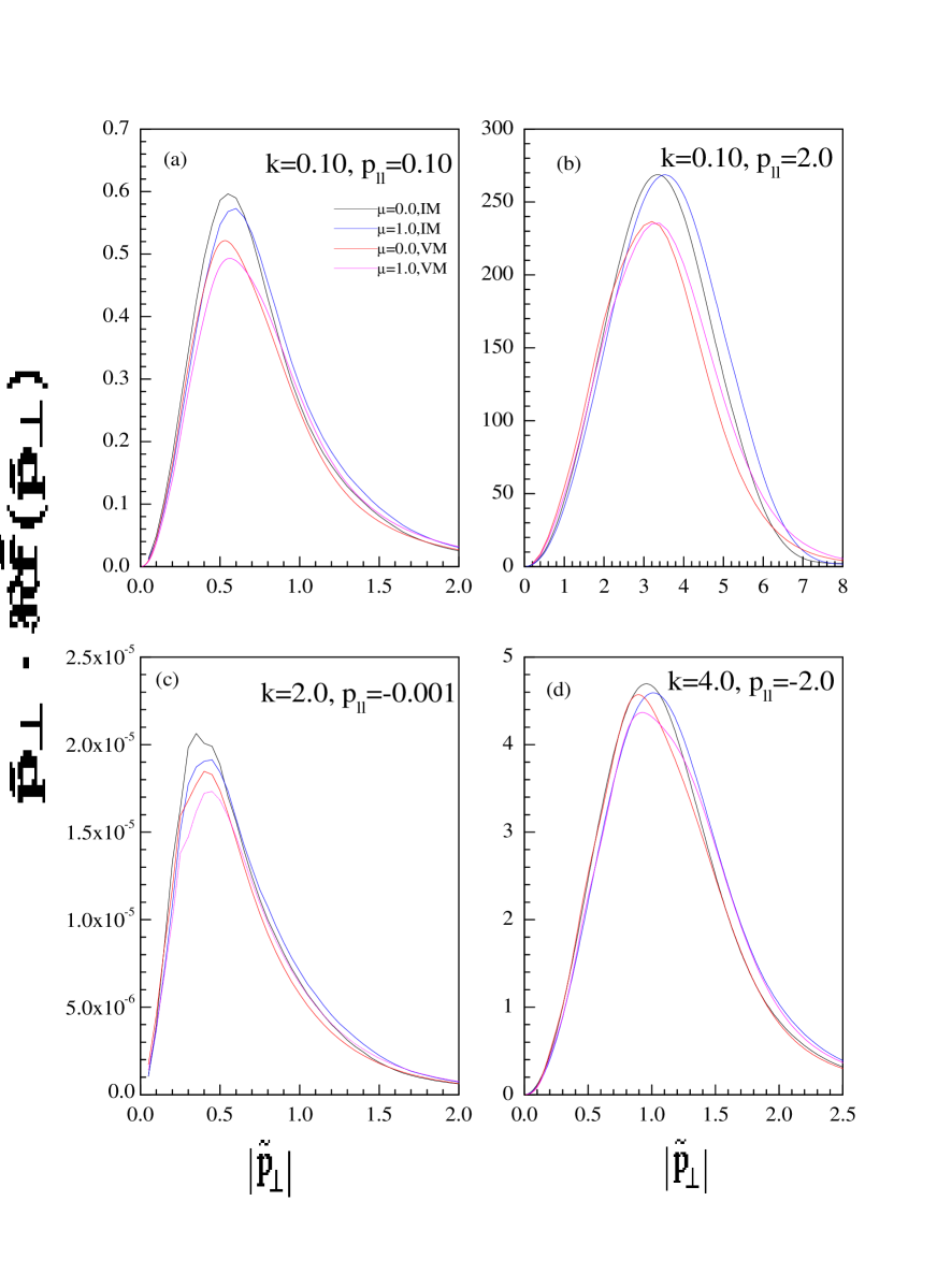
Figure 1: The $2{\bf\tilde{p}_{\perp}}\cdot\Re{\bf\tilde{f}}({\bf\tilde{p}_{\perp}})$ distributions from iteration method (IM) for bremsstrahlung (Figs.(a,b)) and ${\bf aws}$ (Figs.(c,d)) processes. The black curves are for the case of zero density and the blue curves are for finite density with 1.0 GeV quark chemical potential. The corresponding cases from variational method (VM) are shown in red and pink color. The ${p_{\parallel}},k$ values (in GeV) used are shown in figures.

Electromagnetic processes such as photons and dileptons production are considered to be important signals of formation of the quark gluon plasma (QGP) in the relativistic heavy ion collisions. The experimental data by WA98 collaboration [1] of direct photons from Pb+Pb collisions at CERN SPS is of paramount importance which boosted interest in the static emission rates and the convoluted photon yield calculations. A comprehensive review on the theoretical and experimental studies of the photon emission has been given in [2]. The photon emission rates from hot hadron gas, the QGP phase and also the prompt photon emission have been investigated in great detail (see references in [2]). The processes contributing to photon emission from QGP phase at (HTL) effective one loop level are the quark-antiquark annihilation into a photon and a gluon and the absorption of a gluon by a quark (anti quark) emitting photon (see Fig.1 of [2]). The processes of bremsstrahlung and ${\bf aws}$ that arise at effective two loop level contribute at the same order as one loop processes [3]. These processes (see Fig. 5 in [2]) contribute at the leading order $O(\alpha\alpha_{s})$ owing to the collinear singularity that is regularized by the effective thermal masses. The higher order multiple scatterings however can not be ignored as these may also contribute at the same order as the one and two loop processes [4, 5, 6, 7, 8, 9]. Further, multiple soft scatterings of the fermion during photon emission reduce the photon coherence lengths, known as Landau-Pomeranchuk-Migdal (LPM) effect. The photon emission rates are suppressed owing to the LPM effects [5, 6, 7, 8]. Using the hydrodynamical models for the expansion of the plasma and convoluting the expansion with the photon emission rates, one obtains the photon transverse momentum spectrum. These space time evolution of the plasma through QGP, mixed and hadron phases is complicated if the plasma is formed at finite baryon density. These physical conditions of the plasma affect both the basic photon emission rate and the evolution of the plasma and thus the space time integrated photon spectrum. In view of this, the formalism of Aurenche et. al., of photon emission rates at two loop level has been recently extended to a chemically unsaturated plasma at finite baryon density [10]. These emission rates (meaning same as production rates in this work) and the space time (3+1 dimensional) expansion dynamics of the plasma at finite baryon density have been recently reported [11, 12]. The photon spectra have been shown for various cases of plasma at finite baryon density for SPS and RHIC energies and the baryon free case in [12] included the LPM effects.

The photon production rates from bremsstrahlung and the $\bf aws$ processes have been estimated by Aurenche et. al., [3]. In a remarkable simplification, these rates are expressed in terms of simple one dimensional momentum integrals and the dimensionless quantities $J_{T},J_{L}$ [3]. These values are not very sensitive to baryo chemical potential and they weakly depend on the thermal masses for gluon and fermions through $m_{g}^{2}/m_{\infty}^{2}$ [10]. The differential photon emission rate per unit volume of energy $k_{0}$ is given by (denoted by${\cal R}^{0}$ for simplicity of later use),

$${{\cal R}^{0}}_{b,a}=\frac{40\alpha\alpha_{s}}{9\pi^{4}}n_{B}(k_{0})\frac{T}{k^{2}}(J_{T}-J_{L})~{}I_{b,a}(k)$$ (1)

$$I_{b}(k)=\int_{0}^{\infty}dp\left(p^{2}+(p+k)^{2}\right)\left[(n_{f}(p)-n_{f}(p+k))+(\bar{n}_{f}-\bar{n}_{f}(p+k)\right]$$ (2)

$$I_{a}(k)=\int_{0}^{\infty}dp\left(p^{2}+(k-p)^{2}\right)\left[1-\bar{n}_{f}(p)-\bar{n}_{f}(k-p)\right]$$ (3)

In above, the subscripts  $(b,a)$  denote the bremsstrahlung and the $\bf aws$ processes and we consider a two flavor three color case with $\alpha_{s}=0.2$. These rates in Eq. 1 do not include LPM suppression effect. The effects of finite baryon density on the photon emission rates have been discussed in [11] and these results are summerised as follows. The bremsstrahlung radiation is affected whereas the ${\bf aws}$ process is insensitive to the baryon density presence. The bremsstrahlung radiation from quark is enhanced and from anti quark is suppressed at finite baryon density. As mentioned earlier, it has been shown that multiple scatterings during the photon emission for the bremsstrahlung and ${\bf aws}$ processes cannot be ignored. The exchange of a soft gluon of finite thermal mass and the collinear singularity (arising when photon is emitted parallel to quark momentum) regularized by the thermal masses are essentially the factors that make the two loop processes contribute at the same order as the one loop processes. It has been realized [5, 7] that for similar reasons, multiple gluon exchange processes in terms of certain ladder diagrams also contribute to the same order. The diagrammatic analysis of all the processes contributing to the same order has been performed and these contributions have been summed in [7]. This leads to suppression of photon emission rates as shown by the LPM suppression factors in Fig. 7. of [8]. One can also obtain the suppression of the total emission rate by using the empirical expressions in Eq.(1.10) of [8] and the two loop rates of Eq. 1 above without LPM effects. It has been shown that the photon radiation from bremsstrahlung is strongly suppressed to $\sim~{}0.2$ at very low $k/T$ values. The suppression becomes weaker at higher photon energies and approaches $\sim 0.86$ for $k/T>10$. In contrast, the $\bf aws$ is unaffected at low $k/T$ values, but falls almost linearly up to $k/T\sim 10$. The bremsstrahlung from anti quark is same as that of quark for a baryon free case. In the presence of finite baryon density, the bremsstrahlung from quark will be different from the anti quark. Therefore, in order to compare with experimental photon spectra, it is necessary to understand how the suppression factors change with baryon density. The chemical potential dependence of the emission rates are contained in the population functions of the quarks (anti quarks). Further, for comparing with experimental data it is necessary to determine these suppression factors (beyond $k/T\sim 10$) up to $k/T\sim 20$ i.e., $k\sim 5$ GeV for T=0.25GeV case. The differential photon emission rate (denoted by $\cal R$) that includes the LPM effects is given by (for details see [8]),

$${\cal R}_{b,a}=\frac{80\pi T^{3}\alpha\alpha_{s}}{(2\pi)^{3}9\kappa}\int_{-\infty}^{\infty}dp_{\parallel}\left[\frac{p_{\parallel}^{2}+(p_{\parallel}+k)^{2})}{p_{\parallel}^{2}(p_{\parallel}+k)^{2})}\right]n_{f}(k+p_{\parallel})(1-n_{f}(p_{\parallel}))~{}2{\bf\tilde{p}_{\perp}\cdot\Re\tilde{f}(\tilde{p}_{\perp})}$$ (4)

In the above $\kappa=m_{\infty}^{2}/m_{D}^{2}~{}~{}(=\frac{1}{4}~{}~{}~{}\mbox{for}~{}~{}\mu=0~{}~{}~{}\mbox{case})$ and the subscripts $(b,a)$ are for bremsstrahlung and ${\bf aws}$ as in Eq. 1, with different kinematic domains and appropriate distribution functions. The value of $\kappa$ is baryon density dependent and is determined by evaluating these thermal masses as listed in the Table as a function of $\mu_{q}$. In the above equation, $\Re{\bf\tilde{f}(\tilde{p}_{\perp})}$ is the real part of a transverse vector (amplitude) function which consists of the LPM effects due to multiple scatterings. This can be taken as transverse vector ${\bf(\tilde{p}_{\perp})}$ times a scalar function of transverse momentum ${\tilde{p}_{\perp}}$. The sign  $\tilde{}$  denotes the dimensionless quantities in units of Debye mass $m_{D}$ as defined in [8]. The function ${\bf\tilde{p}_{\perp}\cdot\Re\tilde{f}(\tilde{p}_{\perp})}$ is determined by the collision kernels ($\tilde{C}({\bf\tilde{q}_{\perp}})$) in terms of the following integral equation.

$$2{\bf\tilde{p}_{\perp}}=i\delta\tilde{E}({\bf\tilde{p}_{\perp}},p_{\parallel},k){\bf\tilde{f}}({\bf\tilde{p}_{\perp}},p_{\parallel},k)+\int\frac{d^{2}{\bf\tilde{q}_{\perp}}}{(2\pi)^{2}}\left[{\bf\tilde{f}}({\bf\tilde{p}_{\perp}},p_{\parallel},k)-{\bf\tilde{f}}({\bf\tilde{p}_{\perp}+\tilde{q}_{\perp}},p_{\parallel},k)\right]\tilde{C}({\bf\tilde{q}_{\perp}})$$ (5)

$$\tilde{C}({\bf\tilde{q}_{\perp}})=\kappa\int d\tilde{q}_{\parallel}d\tilde{q}^{0}\delta(\tilde{q}^{0}-\tilde{q}_{\parallel})\frac{1}{\tilde{q}}\left[\frac{2}{|\tilde{q}^{2}-\tilde{\Pi}_{L}(\tilde{q}^{0},\tilde{q})|^{2}}+\frac{\left(1-(\tilde{q}^{0}/\tilde{q})^{2}\right)^{2}}{|(\tilde{q}^{0})^{2}-\tilde{q}^{2}-\tilde{\Pi}_{T}(\tilde{q}^{0},\tilde{q})|^{2}}\right]$$ (6)

$$\delta\tilde{E}({\bf\tilde{p}_{\perp}},p_{\parallel},k)=\frac{kT}{2p_{\parallel}(k+p_{\parallel})}\left[\tilde{p}_{\perp}^{2}+\kappa\right]$$ (7)

In above, the $\tilde{\Pi}_{L},\tilde{\Pi}_{T}$ are the longitudinal and transverse parts of (dimensionless) thermal self energies of the gauge fields and $\delta\tilde{E}({\bf\tilde{p}_{\perp}},p_{\parallel},k)$ is the energy difference between the relevant states of the system before and after the photon emission [8]. Based on the sum rules for the thermal gluon spectral functions, Aurenche, Gelis and Zaraket obtained an analytical form for the collision kernel as given by Eq. 44 of [6]. This enormously simplifies the photon emission rate calculations, as it circumvents the need for evaluating the integral in Eq. 6 to obtain the collision kernel. In the present work, we adopt this simple analytical form for the collision kernel, with appropriate factors properly taken care of. We have computed the integral in Eq. 6 for the collision kernel and compared with the analytical form given in [6]. We found these to be agreeing, except near ${\bf\tilde{q}_{\perp}}=0$ where the collision kernel of Eq. 6 falls to zero and can be fitted to another analytical form for use in calculations. This result has been surprising as the analytical form in [6] is based on very general assumptions satisfied for gluon thermal (HTL) self energies and sum rules for its spectral functions. The analytical form of [6] for the full integration region can also be used in the calculations. The divergence of kernel in [6] at ${\bf\tilde{q}_{\perp}}$=0 is compensated by the vector function difference and the ${d^{2}{\bf\tilde{q}_{\perp}}}$ together. Further, use of rationalized momenta in terms of debye mass cancel the $3m_{g}^{2}$ terms in the analytical form given by Aurenche et. al.,. Therefore, the $\tilde{C}({\bf\tilde{q}_{\perp}})$ function just scales as $\kappa$ times the analytical forms which are independent of chemical potentials.

The function ${\bf\tilde{p}_{\perp}\cdot\Re\tilde{f}(\tilde{p}_{\perp})}$ as a function of $|{\bf\tilde{p}_{\perp}}|$ has to be solved self consistently for each set of {$p_{\parallel},k,\kappa,T$} values. In the present work, we have solved the equation by iterations at a fixed temperature of T=0.25GeV and obtained $2{\bf\tilde{p}_{\perp}}\cdot\Re{\bf\tilde{f}}({\bf\tilde{p}_{\perp}})$ distribution. For small $p_{\parallel}$ and $k$ values the iterations converge very fast. For small $k$ and large $p_{\parallel}(>2.5)$ the convergence is slow. The peak positions of these distributions have been obtained for each set of $\{p_{\parallel},k,\kappa\}$. It has been noticed that the peak positions of iteration method ($A_{i}$) can be very well approximated by,

$$A_{i}(p_{\parallel},k)=\left|\frac{1}{p_{\parallel}}-\frac{1}{p_{\parallel}+k}\right|^{\beta}$$ (8)

The value of $\beta$ parameter is, $\beta=-0.32$ for bremsstrahlung and $\bf aws$ away from the $p_{\parallel}$ limits. (The value of $\beta=-0.16$ for $\bf aws$ near the $p_{\parallel}$ limits has been a good approximation.) Further, a lowest cut-off value of $A_{i}^{min}=0.32$ was taken, which is necessary near $p_{\parallel}$ limits or very small $k$ values, especially for $\bf aws$ case. The ${\bf\tilde{f}}$ distributions have been studied for various values of quark chemical potentials ranging from 0-2GeV. It has been found that the peak positions are not very sensitive to the chemical potentials. The dependence of the chemical potential is contained in $\kappa$ factor of the integral equation which weakly depends on $\mu$, as shown on the table. Figure $1(a,b,c,d)$ show the distributions of ${\bf\tilde{p}_{\perp}\cdot\Re\tilde{f}(\tilde{p}_{\perp})}$ for typical cases of $\{k,p_{\parallel},\kappa\}$ values. The Figs. 1(a,b) are for bremsstrahlung and Figs. 1(c,d) are for ${\bf aws}$ with the parameter values shown in figures. The black curves show the results from iterations for zero baryo chemical potential and the blue curves show for the case of $\mu=1.0$GeV. As shown in these figures, the $A_{i}$ values do not change significantly with $\mu$. The $A_{i}$ values are generally less than unity for most parameter values for ${\bf aws}$ case. The empiricism has been derived from a study of several plots of the amplitude function for various parameters and at various stages during iterations. The resulting $2{\bf\tilde{p}_{\perp}}\cdot\Re{\bf\tilde{f}}({\bf\tilde{p}_{\perp}})$ distribution from the iteration method can be used to perform the photon rate calculation using Eq.(4), though the method is not efficient. Results of this method for low photon momentum and high $p_{\parallel}$ values become unreliable when the convergence is poor, though the convergence can be improved by standard methods. However, higher $p_{\parallel}$ values ($p_{\parallel}\geq 10T$) contribute lesser to the emission rate owing to the population functions. Therefore, in the following we adopt a different method for the photon emission rates.

We have followed the variational approach discussed in detail in Eqs. [4.20-4.29] of [8] for solving the integral equation. We found that this method is remarkably simple to solve for the $2{\bf\tilde{p}_{\perp}}\cdot\Re{\bf\tilde{f}}({\bf\tilde{p}_{\perp}})$ distributions, though highly intensive in computing time. The choice of trial functions of [8] do not allow the integrals to be analytically tractable and hence can be computed only numerically. Further, proper choice of the scale constant of the variational method $A_{v}$ is necessary for use in these trial functions. The $A_{v}$ value should be around the peak position of the $2{\bf\tilde{p}_{\perp}}\cdot\Re{\bf\tilde{f}}({\bf\tilde{p}_{\perp}})$ distributions. For this purpose, a constraint integral has been given in Eq. 4.24 of [8] . In the present work, we simply this approach as follows.

(i) The scale constants ($A_{v}$) are taken from empirical expression of Eq. 8, ${\it i.e.,}~{}A_{v}(p_{\parallel},k)=A_{i}^{2}$ for brensstrahlung ,  $A_{v}(p_{\parallel},k)=A_{i}$ for $\bf{aws}$.

(ii) These $A_{i}$ values are already shown to be weakly dependent on baryon density. Therefore the scale constants are taken same as for the $\mu=0$ case.

(iii) The collision kernel of Eq. (6) has been replaced by the analytical forms as mentioned in the last section.

These three considerations grossly simplify the problem and bring out the full advantage of the variational method suggested in [8]. We have calculated the $2{\bf\tilde{p}_{\perp}}\cdot\Re\tilde{f}({\bf\tilde{p}_{\perp}})$ distributions for various sets of {$p_{\parallel},k,\kappa$}. We compared these with the iteration method mentioned earlier. These distributions are shown by red colored curves in Figs. 1(a-d) using the dimension ($N_{r})$  12, of the set of trial functions. The pink curve is the corresponding distributions for $\mu=1$ GeV case. As shown in the figures, the agreement between these two methods is good. This agreement remains valid even for low value of $N_{r}$. At finite baryon density, use of dimension $N_{r}=5~{}or~{}6$ is just sufficient for the photon emission rate calculations using $A_{v}(p_{\parallel},k)$. Further, for a choice of $N_{r}$=12 or 15, these distributions will not be sensitive to the $A_{v}$ values used. This is expected in any basis expansion method for sufficiently large dimension of the model space. Therefore, prudent choice of set of functions and parameters seems necessary to get converging results only for lesser dimensions that render computations easy. This has been verified by comparing the distributions for $N_{r}$=4 using $A_{v}(p_{\parallel},k)$ for a few $\{p_{\parallel},k\}$, with the results for $N_{r}$=12 or 15 using any fixed value of $A_{v}$. It has been observed that use of any constant value of $A_{v}$ with $N_{r}$=8 also gives acceptable results, provided the constant $A_{v}$ value is neither too large nor small as compared to the peak positions. It can be larger by a factor two and can be smaller by a factor of half than the value given by the prescription for $A_{v}(p_{\parallel},k)$. A priori, the $A_{v}$ value for use in calculations for any arbitrary case is not known and therefore the aforesaid prescription serves as a general guideline.

The photon emission rates have been calculated for bremsstrahlung and $\bf aws$ using the variational approach for various values of $\mu$ , as denoted by ${\cal R}_{b},{\cal R}_{a}$ in Eq. 4. The emission rates for effective two loop processes without LPM effects have also been calculated using Eq. 1 and are denoted by ${\cal{R}}^{0}_{b},{\cal{R}}^{0}_{a}$. We obtained the suppression factors as defined by the ratio of the rates from these two methods. However for each $\mu$ value, we normalised the suppression factors to unity for the $\bf aws$ process at very low $k$ value ( $k\approx 0.2T$). The bremsstrahlung suppression versus $k$ for all $\mu$ values are asymptotically normalised to zero density case, ${\it i.e.,}$ at  $k\sim 20T$. These normalization factors are obtained from $f_{b}(\mu),f_{a}(\mu)$ defined in the following equations. The normalised (to zero density) suppression factors ($S_{b},S_{a}$) as functions of $k,\mu$ are thus defined as,

$$S_{b}(k,\mu)=\left(\frac{{\cal{R}}_{b}}{{\cal{R}}^{0}_{b}}\right)_{k}\frac{f_{b}(\mu=0)}{f_{b}(\mu)}~{}~{}~{}~{}\mbox{with}~{}~{}~{}~{}f_{b}(\mu)=\left(\frac{{\cal{R}}_{b}}{{\cal{R}}^{0}_{b}}\right)_{k=20T}$$ (9)

$$S_{a}(k,\mu)=\left(\frac{{\cal{R}}_{a}}{{\cal{R}}^{0}_{a}}\right)_{k}\frac{f_{a}(\mu=0)}{f_{a}(\mu)}~{}~{}~{}~{}\mbox{with}~{}~{}~{}~{}f_{a}=\left(\frac{{\cal{R}}_{a}}{{\cal{R}}^{0}_{a}}\right)_{k=0.2T}$$ (10)

These normalised suppression factors are shown in Figs. 2(a,b), for each $\mu$ (quark chemical potential) as captioned in the figures. The effects of baryon density on these suppression factors is weak only for low baryon density and the qualitatively these are very similar to the results shown in [8]. Our suppression factors agree quite well with the results of [8] for baryon free case. The normalization factors $f_{b},f_{a}$ are shown in the table as a function of quark chemical potential. The values of various thermal masses and $\kappa$ values are also shown in the table. As seen in the table, the normalization factors $f_{a}$ for ${\bf aws}$ are very close to 1.0 showing that the baryon density has no effect. The ${\bf aws}$ suppression factors in Fig. 2(b) also show only weak dependence on baryon density. Therefore in total the ${\bf aws}$ process is insensitive to baryon density and one can use the suppression factors for zero density case for use in photon spectrum calculations. However, for the bremsstrahlung case the density effect is not totally weak. It can be seen from the table that the $f_{b}(\mu)$ value varies considerably for large chemical potential values. The total suppression curves as a function of $k$ for the bremsstrahlung and ${\bf aws}$ at a given $\mu$ are thus given by multiplying with $\frac{f_{b,a}(\mu)}{f_{b,a}(\mu=0)}$ the respective curves in Fig. 2(a,b) to undo the normalization. For low density, one can use the suppression factors as a function of $k$ for zero density case multiplied by a density dependent factors $\frac{f_{b,a}(\mu)}{f_{b,a}(\mu=0)}$. It may be of interest to know from the table that $\kappa f_{b}(\mu)$ is roughly a constant (=0.214) and therefore the density dependent factor can be chosen as $\kappa_{0}/\kappa$. These calculations can be extended to an important case of the plasma conditions at RHIC collision, where the $\kappa$ values can be very different from the values in present study.

Conclusion

The photon emission rates from the quark gluon plasma have been studied considering LPM effects. Self-consistent iterations method has been used to solve the integral equation for the ${\bf\Re\tilde{f}}({\bf\tilde{p}_{\perp}})$ distributions. The peak positions of these distributions have been fitted by an empirical expression for various parameter sets. These peak positions are observed to be rather insensitive to the baryon density. The variational approach has been adopted with some simplifications. Analytical forms for collision kernel have been used in both the iterations and variational methods. The scale constants have been used from empirical expressions from iteration method. The suppression factors for bremsstrahlung and $\bf aws$ have been obtained as a function of photon energy at different baryon densities. The normalised suppression factors are qualitatively similar to the zero baryon density case. The normalization factors show the density dependence for bremsstrahlung. The ${\bf aws}$ process did not show significant density dependence.

Acknowledgements

We acknowledge the fruitful discussions with Dr. S. Kailas and also for initiating us to the use of parallel processors computing system for this study. Dr. A.K. Mohanty is acknowledged for initiating me to these studies and his immense contribution in my career. Dr. A.K. Mohanty and collaborators are specially thanked. We thank Dr. A. Navin for his keen interest in this work. We thank especially the head computer division, BARC. Our sincere thanks to the staff of computer division P.S. Dekne, K. Rajesh, Jagdeesh, P. Saxena and also the operating staff for making available the BARC Anupam parallel processors computing system and constant co-operation during this study. The iteration part of the present study, the resulting peak position parameterization, the emission spectrum calculations have been feasible, thanks to this parallel processors facility.

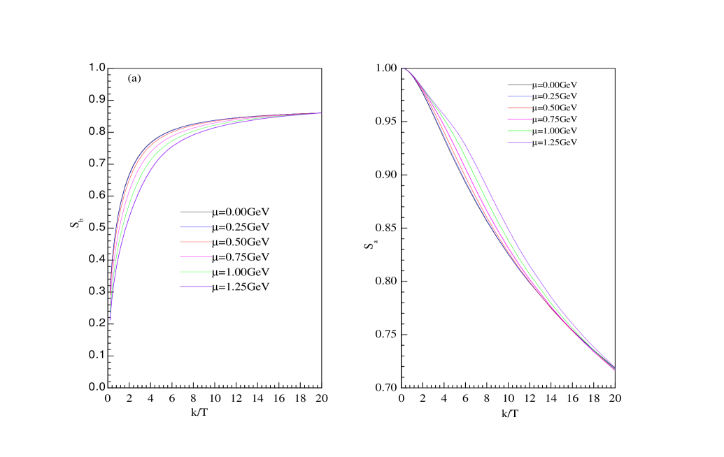
Figure 2: (a) bremsstrahlung and (b) ${\bf aws}$ suppression factors versus photon energy. The suppression factors have been normalised to zero density case asymptotically for bremsstrahlung and for ${\bf aws}$ the normalization is at $k=0.2T$. The true curves at nonzero density can be obtained from the normalization factors given in table, as discussed in text.

$\mu$	$m_{g}^{2}/m_{\infty}^{2}$	$\kappa$	$m_{\infty}^{2}$	$m_{d}^{2}$	$f_{b}$	$f_{a}$
0.00	1.33333	0.25000	0.05236	0.20944	0.85530	0.99382
0.10	1.32802	0.25100	0.05321	0.21199	0.85250	0.99349
0.25	1.30267	0.25589	0.05767	0.22535	0.83952	0.99192
0.50	1.23720	0.26943	0.07358	0.27310	0.80634	0.98780
0.75	1.17435	0.28385	0.10011	0.35268	0.77023	0.98379
1.00	1.12717	0.29572	0.13724	0.46408	0.73468	0.98074
1.25	1.09434	0.30460	0.18500	0.60736	0.70158	0.97860
1.50	1.07173	0.31102	0.24332	0.78233	0.67098	0.97711
1.75	1.05588	0.31569	0.31236	0.98944	0.64143	0.97607
2.00	1.04454	0.31912	0.39182	1.22782	0.61527	0.97532

References

- [1] M. M. Agarwalet. al., . WA98 Collaboration nucl-ex/0006007 ; Phys. Rev. Lett. 85, 3595 (2000)
- [2] Thomas Peitzman and Markus H. Thoma, hep-ph/0111114.
-
[3]
P. Aurenche, F. Gelis, H. Zaraket and R. Kobes , Phys.
Rev. D58 085003 (1998), [hep-ph/9804224] ;
P. Aurenche, F. Gelis, R. Kobes and E. Petitgirard, Phys. Rev. D54 5274 (1996) [hep-ph/9604398]; Z. Phys. ,315 (1996). - [4] P. Aurenche, F. Gelis, R. Kobes and H. Zaraket, Phys. Rev. D61 116001 (2000) [hep-ph/9911367]
- [5] P. Aurenche, F. Gelis, and H. Zaraket, Phys. Rev. D62 096012 (2000) [hep-ph/0003326]
- [6] P. Aurenche, F. Gelis, and H. Zaraket, hep-ph/0204146
- [7] Peter Arnold, Guy D. Moore and Laurence G. Yaffe, JHEP 0112 (2001) 009, [hep-ph/0111107]
- [8] Peter Arnold, Guy D. Moore and Laurence G. Yaffe, JHEP 0111 (2001) 057, [hep-ph/0109064].
- [9] Peter Arnold, Guy D. Moore and Laurence G. Yaffe, hep-ph/0204343.
- [10] D. Dutta, S. V. S. Sastry, A. K. Mohanty, K. Kumar and R. K. Choudhury, hep-ph/0104134 ; Submitted to Nucl. Phys A
- [11] D. Dutta, S. V. S. Sastry, A. K. Mohanty, K. Kumar and R. K. Choudhury, Presented in ICPA-QGP-’01, Nov 2001, held at Jaipur, India, Conf. proceedings to appear in Pramana.
- [12] S. V. S. Sastry, D. Dutta, A. K. Mohanty and D. K. Srivastava, hep-ph/0204250.